Yield-SAFE model improvements. Milestone Report 29 (6.4)

AGFORWARD (Grant Agreement N° 613520) is co-funded by the European Commission, Directorate General for Research & Innovation, within the 7th Framework Programme of RTD. The views and opinions expressed in this report are purely those of the writers and may not in any circumstances be regarded as

Yield-SAFE Model Improvements

Project name AGFORWARD (613520)

Work-package 6: Field- and Farm-scale Evaluation of Innovations Deliverable Milestone 29 (6.4): Yield-SAFE model improvements Date of report 20 April 2016; updated 16 June 2016

Authors João Palma, Anil Graves, Josep Crous-Duran J, Matt Upson, Joana A Paulo,

Tania S

Oliveira, Silvestre Garcia de Jalón, Paul Burgess Contact [email protected]

Approved Paul Burgess (5 July 2016)

Contents 1 Context ... 2 2 Crop ... 2 3 Tree ... 5 4 Soil ... 14 5 Livestock ... 20 6 Yield-SAFE interfaces... 22 7 References ... 27

Appendix A. Information to use WebYield-SAFE and the source link ... 29

1 Context

The AGFORWARD research project (January 2014-December 2017), funded by the European Commission, is promoting agroforestry practices in Europe that will advance sustainable rural development. The project has four objectives:

1. to understand the context and extent of agroforestry in Europe,

2. to identify, develop and field-test innovations (through participatory research) to improve the benefits and viability of agroforestry systems in Europe,

3. to evaluate innovative agroforestry designs and practices at a field-, farm- and landscape scale, and

4. to promote the wider adoption of appropriate agroforestry systems in Europe through policy development and dissemination.

The third objective is addressed partly by work-package 6 which focuses on the field- and farm-scale evaluation of agroforestry systems and innovations. One of the models being used for simulating agroforestry systems is Yield-SAFE (van der Werf et al. 2007), developed under the SAFE project (Dupraz et al. 2005).

The Yield-SAFE model is a parameter-sparse, process-based dynamic model for predicting resource capture, growth, and production in agroforestry systems that has been frequently used by various research organisations in recent years.

Within the AGFORWARD project, the model has been enhanced to more accurately predict the delivery of ecosystem services provided by agroforestry systems relative to forestry and arable systems. This report also summarizes the new developments made in the model which were partially implemented during AGFORWARD modelling workshops held in 1) Monchique in Portugal in May 2015, 2) Kriopigi in Greece in June 2015, 3) Lisbon in Portugal in November 2015 and 4) Lisbon in February 2016.

This report has been partially published as:

Palma JHN, Graves AR, Crous-Duran J, Paulo JA, Oliveira TS, Garcia de Jalon S, Kay S, Burgess PJ, (2016), Keeping a parameter-sparse concept in agroforestry modeling while integrating new processes and dynamics: New developments in Yield-SAFE, III EURAF Conference, Montpellier 23-25 May 2016.

2 Crop

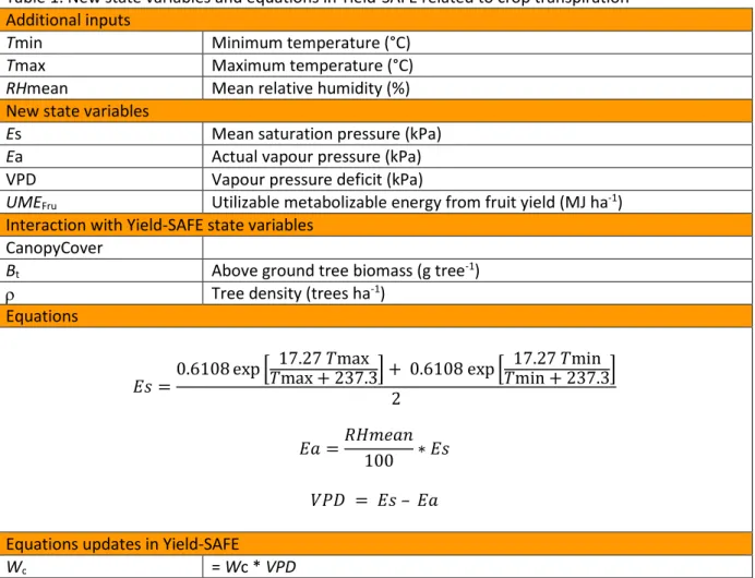
2.1 Transpiration

The crop water uptake state variable (Wc) was a simple relationship between the daily biomass growth and the water use efficiency parameter. Formerly, for the same crop, there was a need to increase the water needed to produce the same amount of biomass (𝑐) for drier Mediterranean climates relative to more humid Atlantic climates. This dual calibration was required mainly due to a higher vapour pressure deficit (VPD) in drier regions. The water use efficiency of the crop is now a reference for a VPD of 1 kPa while the water use responds to the daily VPD calculations. The decision to link the water uptake to VPD led to the increase of climate inputs (minimum temperature, maximum temperature and relative humidity), but the use of these climate variables also increased the potential to assess other aspects of the ecosystem services provided by agroforestry systems. The integration of these relationships was based on Allen et al. (1998) for the VPD calculations and

Tanner and Sinclair (1983) for the water use relationship to VPD. The new state variable and equations used in Yield-SAFE related to crop transpiration are provided in Table 1.

Table 1. New state variables and equations in Yield-SAFE related to crop transpiration Additional inputs

Tmin Minimum temperature (°C) Tmax Maximum temperature (°C) RHmean Mean relative humidity (%) New state variables

Es Mean saturation pressure (kPa)

Ea Actual vapour pressure (kPa)

VPD Vapour pressure deficit (kPa)

UMEFru Utilizable metabolizable energy from fruit yield (MJ ha-1) Interaction with Yield-SAFE state variables

CanopyCover

Bt Above ground tree biomass (g tree-1)

 Tree density (trees ha-1₎

Equations 𝐸𝑠 =0.6108 exp [ 17.27 𝑇max 𝑇max + 237.3] + 0.6108 exp [ 17.27 𝑇min 𝑇min + 237.3] 2 𝐸𝑎 =𝑅𝐻𝑚𝑒𝑎𝑛 100 ∗ 𝐸𝑠 𝑉𝑃𝐷 = 𝐸𝑠 – 𝐸𝑎 Equations updates in Yield-SAFE

2.2 Maintenance respiration

Unlike annual crops, grass is a perennial crop. As Yield-SAFE did not previously account for crop respiration, the original Yield-SAFE set-up can result in an unrealistic yearly annual accumulation of biomass in the system if the grass was not harvested. Therefore a crop respiration rate was added for the modelling of grass, enabling the reduction of biomass when the daily growth is lower than the carbon used for biomass maintenance (Table 2). The integration was made using the equation proposed by Thornley (1970).

Table 2. New state variables and equations in Yield-SAFE related to crop maintenance respiration Additional parameters

Kmainc_m Maintenance coefficient representing the amount of carbon respired to maintain existing biomass (g-1_g-1₎

Kmainc_g Amount of carbon respired per unit of carbon used in growth (g-1 g-1) New state variables

Rc Crop maintenance respiration (g m

-2₎ Interaction with Yield-SAFE state variables

Bc Crop biomass (g m-2)

𝑑𝐵𝑐𝐴𝑐𝑡 Actual growth (g m

-2₎ Equations

𝑅𝑐 𝑘 = 𝐾𝑚𝑎𝑖𝑛𝑐_𝑚 𝐵𝑐 𝑘−1+ 𝐾𝑚𝑎𝑖𝑛𝑐_𝑔 𝑑𝐵𝑐𝐴𝑐𝑡_𝑘−1 k-1 denotes the previous day

Equations updates in Yield-SAFE

𝑑𝐵𝑐𝐴𝑐𝑡 = 𝑑𝐵𝑐

𝐴𝑐𝑡 _{– Rc}

Note: Values of Kmain_m = 0.037 and Kmain_g = 0.54 can be used for grassland as suggested by Reekie and Redmann (1987).

2.3 Carbon inputs to soil

After harvest, crop roots are considered as a carbon input to the soil. Similarly to the new fine root tree component, crop root biomass is estimated as a root-to-shoot ratio, which by using a carbon content in roots, will estimate the carbon being added to the soil in the day of harvest (Table 3). Table 3. New state variables and equations in Yield-SAFE related to carbon inputs to soil

Additional parameters:

RSRc Root to shoot ratio (0-1)

fCCRc _{proportion of carbon content in crop roots (0-1)} New state variables

BcRoots Biomass of crop roots (g m-2)

CRMc Carbon content in crop roots (kgC ha-1) Interaction with Yield-SAFE state variables

Bc Above ground crop biomass (g m-2)

Equations

𝐵𝑐𝑅𝑜𝑜𝑡𝑠= 𝐵𝑐∗ 𝑅𝑆𝑅𝑐

𝐶𝑅𝑀𝑐= 𝐵𝑐𝑅𝑜𝑜𝑡𝑠∗ 𝑓𝐶𝐶𝑅𝑐

Equations updates in Yield-SAFE None

3 Tree

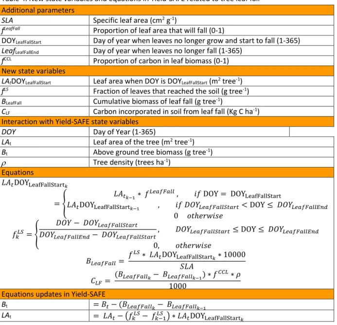
3.1 Leaf fall

Trees can affect crop production negatively through competition for light, nutrients and water, as well as positively through increased input of biomass from leaves and roots that often enhance nutrient cycling (Rao et al. 1998). Although growth impact nutrients (i.e. N, P, K) are not implemented in Yield-SAFE, carbon dynamics are now simulated. Leaf fall and leaf biomass is now incorporated in the soil carbon model as plant input material in the soil carbon dynamics module (Section 4.2) using the specific leaf area (SLA). The biomass of leaves to fall depends on i) the proportion of leaf area that will fall (values <1 can define perennials), ii) the day of year when leaves start to fall (DOYLeafFallStart) and iii) the number of days leaves are falling (LeafFallingDays). The amount of biomass falling from the tree is evenly distributed between LeafFallingDays, and is subtracted from the tree biomass state variable. The carbon from leaf fall (CLF) is given by a parameter (fCCL) defining the fraction of carbon content in the biomass of leaves, which converted to a per hectare basis becomes the input to the soil carbon module (Table 4).

Table 4. New state variables and equations in Yield-SAFE related to tree leaf fall Additional parameters

SLA Specific leaf area (cm2 _g-1₎

fLeafFall _{Proportion of leaf area that will fall (0-1)}

DOYLeafFallStart Day of year when leaves no longer grow and start to fall (1-365)

LeafLeafFallEnd Day of year when leaves no longer fall (1-365)

fCCL _{Proportion of carbon in leaf biomass (0-1)} New state variables

LAtDOYLeafFallStart Leaf area when DOY is DOYLeafFallStart (m2 tree-1)

fLS _{Fraction of leaves that reached the soil (g tree}-1₎

BLeafFall Cumulative biomass of leaf fall (g tree-1)

CLF Carbon incorporated in soil from leaf fall (Kg C ha-1) Interaction with Yield-SAFE state variables

DOY Day of Year (1-365)

LAt Leaf area of the tree (m2 tree-1)

Bt Above ground tree biomass (g tree-1)

 Tree density (trees ha-1₎

Equations

𝐿𝐴𝑡DOYLeafFallStart_𝑘

= {

𝐿𝐴𝑡_𝑘−1∗ 𝑓𝐿𝑒𝑎𝑓𝐹𝑎𝑙𝑙 , 𝑖𝑓 DOY = DOYLeafFallStart

𝐿𝐴𝑡DOYLeafFallStart𝑘−1 , 𝑖𝑓 𝐷𝑂𝑌𝐿𝑒𝑎𝑓𝐹𝑎𝑙𝑙𝑆𝑡𝑎𝑟𝑡 < DOY ≤ 𝐷𝑂𝑌𝐿𝑒𝑎𝑓𝐹𝑎𝑙𝑙𝐸𝑛𝑑 0 𝑜𝑡ℎ𝑒𝑟𝑤𝑖𝑠𝑒 𝑓_𝑘𝐿𝑆= { 𝐷𝑂𝑌 − 𝐷𝑂𝑌𝐿𝑒𝑎𝑓𝐹𝑎𝑙𝑙𝑆𝑡𝑎𝑟𝑡 𝐷𝑂𝑌𝐿𝑒𝑎𝑓𝐹𝑎𝑙𝑙𝐸𝑛𝑑− 𝐷𝑂𝑌𝐿𝑒𝑎𝑓𝐹𝑎𝑙𝑙𝑆𝑡𝑎𝑟𝑡 , 𝐷𝑂𝑌𝐿𝑒𝑎𝑓𝐹𝑎𝑙𝑙𝑆𝑡𝑎𝑟𝑡≤ DOY ≤ 𝐷𝑂𝑌𝐿𝑒𝑎𝑓𝐹𝑎𝑙𝑙𝐸𝑛𝑑 0, 𝑜𝑡ℎ𝑒𝑟𝑤𝑖𝑠𝑒 𝐵𝐿𝑒𝑎𝑓𝐹𝑎𝑙𝑙 = 𝑓𝐿𝑆∗ 𝐿𝐴𝑡DOYLeafFallStart𝑘∗ 10000 𝑆𝐿𝐴 𝐶𝐿𝐹 = (𝐵𝐿𝑒𝑎𝑓𝐹𝑎𝑙𝑙_𝑘− 𝐵𝐿𝑒𝑎𝑓𝐹𝑎𝑙𝑙_𝑘−1) ∗ 𝑓𝐶𝐶𝐿∗ 𝜌 1000 Equations updates in Yield-SAFE

Bt = 𝐵𝑡− (𝐵𝐿𝑒𝑎𝑓𝐹𝑎𝑙𝑙_𝑘− 𝐵𝐿𝑒𝑎𝑓𝐹𝑎𝑙𝑙_𝑘−1

LAt = 𝐿𝐴_𝑡− (𝑓_𝑘𝐿𝑆− 𝑓_𝑘−1𝐿𝑆 ) ∗ 𝐿𝐴_𝑡DOY_{LeafFallStart}

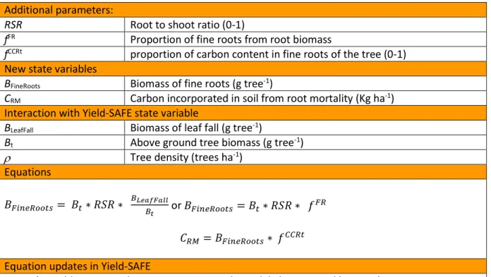
3.2 Fine root mortality

Fine root mortality also adds plant material to the soil carbon module. However the turnover rate depends on various factors occurring in soil conditions, e.g. water logging, soil temperature, nutrient availability, mycorrhizae symbiosis, tree physiology and phenology (Pregitzer 2002). Yield-SAFE simplifies this dynamics with an approach that all fine roots will die and become incorporated in soil for decomposing. The timing of the incorporation of fine roots is also complex and arguable but Yield-SAFE simplifies this by linking to the leaf fall period on the basis of “biomass balance” between above and belowground, i.e. fine roots biomass is calculated at the time when leaf fall starts, and root mortality follows the same time pattern of leaf fall.

Root biomass now is estimated as a root-to-shoot ratio, frequently used values are 0.2 and 0.25 for conifers and broadleaf respectively (IPCC 2006). Some literature supports that fine roots can be a proportion of root biomass in the same proportion that leaves have in aboveground biomass (Madeira et al. 2002), therefore in Yield-SAFE, fine roots can be estimated either based on the proportion of leaves to tree aboveground biomass or, alternatively, a user can define the proportion of fine roots in the belowground biomass (Table 5).

Table 5. New state variables and equations in Yield-SAFE related to tree fine root mortality Additional parameters:

RSR Root to shoot ratio (0-1)

fFR _{Proportion of fine roots from root biomass}

fCCRt _{proportion of carbon content in fine roots of the tree (0-1)} New state variables

BFineRoots Biomass of fine roots (g tree-1)

CRM Carbon incorporated in soil from root mortality (Kg ha-1) Interaction with Yield-SAFE state variable

BLeafFall Biomass of leaf fall (g tree-1)

Bt Above ground tree biomass (g tree-1)

 Tree density (trees ha-1₎

Equations 𝐵𝐹𝑖𝑛𝑒𝑅𝑜𝑜𝑡𝑠 = 𝐵𝑡∗ 𝑅𝑆𝑅 ∗ 𝐵_{𝐿𝑒𝑎𝑓𝐹𝑎𝑙𝑙} 𝐵_𝑡 or 𝐵𝐹𝑖𝑛𝑒𝑅𝑜𝑜𝑡𝑠= 𝐵𝑡∗ 𝑅𝑆𝑅 ∗ 𝑓 𝐹𝑅 𝐶𝑅𝑀= 𝐵𝐹𝑖𝑛𝑒𝑅𝑜𝑜𝑡𝑠∗ 𝑓𝐶𝐶𝑅𝑡

Equation updates in Yield-SAFE

3.3 Cork

If the user is simulating cork oak stands (Quercus suber L.) and needs to estimate cork production, we have set the model to estimate cork production based on equations developed by Paulo and Tomé (2014) for the estimation of virgin cork weight (cork resulting from the first cork extraction) and by Paulo and Tomé (2010) for the estimation of non-virgin or mature cork (Table 6).

Table 6. New state variables and equations in Yield-SAFE related to cork production Additional parameters

DOYdebarking Day of year when debarking takes place (1-365)

dcoef Debarking coefficient (ratio between vertical debarking height and perimeter at breast height with cork)

Hdebark Vertical debarking height (cm)

PBHmin Minimum perimeter at breast height for debarking (cm)

debarkCalendar Years of age for each cork extraction (years,years,years, …) Agestartdeb Starting debarking tree age

New state variables

d Diameter at breast height with virgin cork (cm)

Debarknr Sequential number of debarking event (0,1, …) Daydebark Day of debarking (0 = true or 1 = false)

wcv Dry weight of extracted virgin cork (kg)

wca Dry weight of extracted mature cork (kg)

wc Dry weight of extracted cork (kg)

Interaction with Yield-SAFE state variables

dbh Tree diameter at breast height (without cork) (cm)

DOY Day of Year (1-365)

Bt Above ground tree biomass (g tree-1)

Equations 𝑑 = { 𝑑 = 𝑑𝑏ℎ + 1.5276 0.8321 , 𝑖𝑓 𝑑𝑏ℎ > 7.5 𝑑 = 𝑑𝑏ℎ, 𝑜𝑡ℎ𝑒𝑟𝑤𝑖𝑠𝑒 𝐷𝑎𝑦𝑑𝑒𝑏𝑎𝑟𝑘= { 1, 𝑖𝑓 𝑑 > 𝑃𝐵𝐻𝑚𝑖𝑛 𝜋 𝑎𝑛𝑑 𝐷𝑂𝑌 = 𝐷𝑂𝑌𝑑𝑒𝑏𝑎𝑟𝑘𝑖𝑛𝑔 0, 𝑜𝑡ℎ𝑒𝑟𝑤𝑖𝑠𝑒 𝐷𝑒𝑏𝑎𝑟𝑘𝑛𝑟 = { 𝐷𝑒𝑏𝑎𝑟𝑘𝑛𝑟+ 1, 𝑖𝑓 𝐷𝑂𝑌 = 𝐷𝑂𝑌𝑑𝑒𝑏𝑎𝑟𝑘𝑖𝑛𝑔 𝐷𝑒𝑏𝑎𝑟𝑘𝑛𝑟, 𝑜𝑡ℎ𝑒𝑟𝑤𝑖𝑠𝑒 𝑤𝑐𝑣 = {−19.6723 + 0.00734 𝑑𝑏ℎ 2_{+ 4.25364 ln(dcoef), 𝑖𝑓 𝐷𝑒𝑏𝑎𝑟𝑘} 𝑛𝑟= 1 𝑎𝑛𝑑 𝑖𝑓 𝐷𝑂𝑌 = 𝐷𝑂𝑌𝑑𝑒𝑏𝑎𝑟𝑘𝑖𝑛𝑔 0, 𝑜𝑡ℎ𝑒𝑟𝑤𝑖𝑠𝑒 𝑤𝑐𝑎 = { 0.0203 𝑑𝑏ℎ 1.9843_{, 𝑖𝑓 𝐷𝑒𝑏𝑎𝑟𝑘} 𝑛𝑟 > 1 𝑎𝑛𝑑 𝑖𝑓 𝐷𝑂𝑌 = 𝐷𝑂𝑌𝑑𝑒𝑏𝑎𝑟𝑘𝑖𝑛𝑔 0, 𝑜𝑡ℎ𝑒𝑟𝑤𝑖𝑠𝑒 wc = wcv + wca Equations updates in Yield-SAFE

The model simulates the first debarking when the tree diameter is above a certain threshold of a perimeter at breast height (PBHmin; cm). For example, PBHmin is defined by Portuguese law as 70 cm. The interval between consecutive cork extraction events (cork debarking rotation) is defined for 9 years, as this is the minimum interval allowed by Portuguese and Spanish national legislation and is frequently used by managers, although this calendar can be defined by the user (debarkCalendar). After each cork extraction, cork biomass is subtracted from the tree biomass state variable.

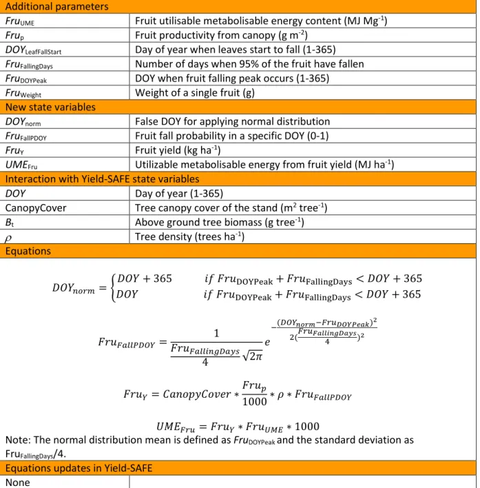
3.4 Fruit production

Fruit production is now considered as a linear relationship between the tree leaf area and a parameter defining the productivity (Table 7). The fruit is defined in terms of energy content and the falling period simulated as a normal distribution. This will enable the estimation of livestock carrying capacity and also the number of sequential grazing days considering the fruit energetic availability. Table 7. New state variables and equations in Yield-SAFE related to fruit production

Additional parameters

FruUME Fruit utilisable metabolisable energy content (MJ Mg-1)

Frup Fruit productivity from canopy (g m-2)

DOYLeafFallStart Day of year when leaves start to fall (1-365)

FruFallingDays Number of days when 95% of the fruit have fallen

FruDOYPeak DOY when fruit falling peak occurs (1-365)

FruWeight Weight of a single fruit (g) New state variables

DOYnorm False DOY for applying normal distribution

FruFallPDOY Fruit fall probability in a specific DOY (0-1)

FruY Fruit yield (kg ha-1)

UMEFru Utilizable metabolisable energy from fruit yield (MJ ha-1) Interaction with Yield-SAFE state variables

DOY Day of year (1-365)

CanopyCover Tree canopy cover of the stand (m2 _tree-1₎

Bt Above ground tree biomass (g tree-1)

 Tree density (trees ha-1₎

Equations 𝐷𝑂𝑌𝑛𝑜𝑟𝑚= { 𝐷𝑂𝑌 + 365 𝑖𝑓 𝐹𝑟𝑢DOYPeak+ 𝐹𝑟𝑢FallingDays< 𝐷𝑂𝑌 + 365 𝐷𝑂𝑌 𝑖𝑓 𝐹𝑟𝑢DOYPeak+ 𝐹𝑟𝑢FallingDays< 𝐷𝑂𝑌 + 365 𝐹𝑟𝑢𝐹𝑎𝑙𝑙𝑃𝐷𝑂𝑌= 1 𝐹𝑟𝑢𝐹𝑎𝑙𝑙𝑖𝑛𝑔𝐷𝑎𝑦𝑠 4 √2𝜋 𝑒 −(𝐷𝑂𝑌𝑛𝑜𝑟𝑚−𝐹𝑟𝑢𝐷𝑂𝑌𝑃𝑒𝑎𝑘)2 2(𝐹𝑟𝑢𝐹𝑎𝑙𝑙𝑖𝑛𝑔𝐷𝑎𝑦𝑠 4 )2 𝐹𝑟𝑢𝑌= 𝐶𝑎𝑛𝑜𝑝𝑦𝐶𝑜𝑣𝑒𝑟 ∗ 𝐹𝑟𝑢𝑝 1000∗ 𝜌 ∗ 𝐹𝑟𝑢𝐹𝑎𝑙𝑙𝑃𝐷𝑂𝑌 𝑈𝑀𝐸𝐹𝑟𝑢= 𝐹𝑟𝑢𝑌∗ 𝐹𝑟𝑢𝑈𝑀𝐸∗ 1000

Note: The normal distribution mean is defined as FruDOYPeak and the standard deviation as FruFallingDays/4.

Equations updates in Yield-SAFE None

Carrying capacity sequential days based on fruit production

Fruit production is an important energetic asset for some tree species. In this improvement, the fruit production is linked to its energy content and to the livestock energy requirements. There are two main indicators: i) the number of sequential days the daily tree fruit production can handle one livestock unit and ii) given a livestock carrying capacity provided by the user, how many sequential days the system can provide.

Table 8. New state variables and equations in Yield-SAFE related to the carrying capacity sequential days based on fruit production

Additional parameters

FruUME Fruit utilisable metabolisable energy content (MJ Mg-1)

LMER Livestock unit utilisable metabolisable energy requirement (MJ d-1₎

SLMER Selected livestock utilisable metabolisable energy requirement (MJ d-1₎

SLDCC Selected livestock carrying capacity ULU User defined livestock units (LU ha -1₎ New state variables

UMEFru Daily Utilizable metabolisable energy from fruit yield (MJ ha-1)

UMEFruY Yearly cumulative utilizable metabolisable energy from fruit yield (MJ ha-1₎

CCFruLU Carrying capacity of livestock units from fruit yield (LU ha-1)

CCFruSLU Carrying capacity of selected livestock from fruit yield (SL ha-1)

CCSDFru Counter for sequential carrying capacity above 1 livestock unit from fruit yield (nr days)

CCSDFruyr Carrying capacity sequential days from fruit yield (days year -1)

SLCCSDFru Counter for sequential carrying capacity above 1 selected livestock unit from fruit yield (nr days)

SLCCSDFruyr Selected livestock carrying capacity sequential days from fruit yield (days year -1₎

SDULUFru Counter for sequential days for user defined livestock units from fruit yield, (nr days)

SDULUFruyr Sequential days for user defined livestock units from fruit yield (days year -1₎

Interaction with Yield-SAFE state variables

FruFallPDOY Fruit fall probability in a specific DOY (0-1) (see Section 3.4)

FruY Fruit yield (kg ha-1) (see Section 3.4) Equations 𝑈𝑀𝐸𝐹𝑟𝑢= 𝐹𝑟𝑢𝑌∗ 𝐹𝑟𝑢𝑈𝑀𝐸 1000 𝑈𝑀𝐸𝐹𝑟𝑢𝑌= { 0 , 𝑖𝑓 𝐹𝑟𝑢𝐹𝑎𝑙𝑙𝑃𝐷𝑂𝑌≤ 0.00001 𝑈𝑀𝐸Fru+ 𝑈𝑀𝐸Fru−1 , 𝑖𝑓 𝐹𝑟𝑢𝐹𝑎𝑙𝑙𝑃𝐷𝑂𝑌> 0.00001 𝐶𝐶𝐹𝑟𝑢𝐿𝑈 = 𝑈𝑀𝐸𝐹𝑟𝑢 𝐿𝑀𝐸𝑅 𝐶𝐶𝐹𝑟𝑢𝑆𝐿𝑈= 𝑈𝑀𝐸𝐹𝑟𝑢 𝑆𝐿𝑀𝐸𝑅

𝐶𝐶𝑆𝐷𝐹𝑟𝑢𝑘 = { 𝐶𝐶𝑆𝐷𝐹𝑟𝑢𝑘−1 + 1 , 𝑖𝑓 𝐶𝐶FruLU≥ 1 0 , 𝑖𝑓 𝐶𝐶FruLU< 1 𝐶𝐶𝑆𝐷𝐹𝑟𝑢𝑦𝑟 = 𝑀𝑎𝑥𝐷𝑂𝑌=1𝐷𝑂𝑌=365 𝐶𝐶𝑆𝐷𝐹𝑟𝑢 𝑆𝐿𝐶𝐶𝑆𝐷𝐹𝑟𝑢𝑘{ 𝑆𝐿𝐶𝐶𝑆𝐷𝐹𝑟𝑢𝑘−1 + 1 , 𝑖𝑓 𝐶𝐶𝐹𝑟𝑢SLU ≥ 1 0 , 𝑖𝑓 𝐶𝐶𝐹𝑟𝑢SLU < 1 𝑆𝐿𝐶𝐶𝑆𝐷𝐹𝑟𝑢𝑦𝑟= 𝑀𝑎𝑥𝐷𝑂𝑌=1𝐷𝑂𝑌=365 𝑆𝐿𝐶𝐶𝑆𝐷𝐹𝑟𝑢 𝑆𝐷𝑈𝐿𝑈𝐹𝑟𝑢𝑘{ 𝑆𝐷𝑈𝐿𝑈𝑘−1 + 1 , if 𝐶𝐶𝐹𝑟𝑢LU ≥ 𝑈𝐿𝑈 0 , if 𝐶𝐶𝐹𝑟𝑢LU < 𝑈𝐿𝑈 𝑆𝐷𝑈𝐿𝑈𝐹𝑟𝑢𝑦𝑟= 𝑀𝑎𝑥𝐷𝑂𝑌=1𝐷𝑂𝑌=365 𝑆𝐷𝑈𝐿𝑈𝐹𝑟𝑢

3.5 Water assimilation by roots

This module introduces a new state variable 𝜑 which determines the ability of trees to assimilate water (Table 9). 𝜑is a factor that moderates growth by limiting the variable 𝑊𝑡. This modifier

considers an extinction coefficient governing the absorption of water (kr), the length of fine root per gram (r), and a ration of structural root mass to the above ground biomass (𝜋𝑠𝑟). These parameters

were initially set to values of 𝑘𝑟 = 0.00007, 𝑟 = 30/6378, and 𝜋𝑠𝑟 = 0.22. The latter two were

based on empirical measurements taken at the Silsoe agroforestry trial in 2011 for 19 year old poplar trees. The parameter 𝑘𝑟 was adjusted to achieve a fit between modelled and actual data.

Note that these parameters were introduced along with changes to the soil profile and other tree parameters. A full explanation is given by Upson (2014).

Table 9. New state variables and equations in Yield-SAFE related to water assimilation by roots Additional parameters

kr Extinction coefficient governing the absorption of water per unit of root length (0-1)

r Length of fine root per mass of structural root (m g-1_). 𝜋𝑠𝑟 Ratio of structural root mass to aboveground biomass (0-1)

New state variables

𝜑 Modifier for water assimilation (0-1) Interaction with Yield-SAFE state variables

Bt Above ground tree biomass (g tree-1₎

Ft Water uptake by trees (mm)

Equations

𝜑 = 1 − 𝑒𝐵𝑡𝜋𝑠𝑟𝑟𝑘𝑟 Equations updates in Yield-SAFE

Ft = Ft * 𝜑

Note: If this improvement is causing problems in the usage, 𝑟 (the length of fine root per gram of structural root) can be set to a high value e.g. 50 000 m g-1_.

3.6 Tree effects on microclimate (temperature and wind)

Combining woody perennial and annual crop species modifies microclimatic factors such as wind speed air and understorey temperature, relative humidity, radiation and saturation deficit, and hence evapotranspiration (Luedeling et al. 2016; Muthuri et al. 2014). The effects of trees on temperature and wind speed can now be taken into consideration in Yield-SAFE.

Effects on temperature

Tree canopies not only reduce temperature in summer but also increase temperature in winter and reduce evapotranspiration (Gill and Abrol, 1993; Shanker et al. 2005). For example Gill et al. 1990 (in Dagar et al. 2013) and Gill and Abrol 1993 found that under an Acacia nilotica canopy, the mean air temperature was lowered by 2-5°C during summer and increased 2-4°C in winter.

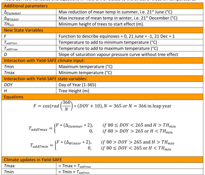
A modifier was introduced in Yield-SAFE to change the temperature when tree height reaches a certain threshold (i.e. 4 m) and when the tree leaves are present (Table 10). Assuming a northern hemisphere, the modifier starts reducing temperature from 21 March with a maximum on 21 June before declining to zero on 21 September. From this date, the modifier increases the temperature until 21 December before declining again to 21 March.

Table 10. New variables and equations in Yield-SAFE related to the effect of trees on temperatures Additional parameters

∆𝑆𝑢𝑚𝑚𝑒𝑟 Max reduction of mean temp in summer, i.e. 21st June (°C)

∆𝑊𝑖𝑛𝑡𝑒𝑟 Max increase of mean temp in winter, i.e. 21st December (°C)

THmin Minimum height of trees to start effect (m). New State Variables

F Function to describe equinoxes = 0, 21 June = -1, 21 Dec = 1 TaddTmin Temperature to add to minimum temperature (°C)

TaddTmax Temperature to add to maximum temperature (°C)

D Slope of saturation vapour pressure curve without tree effect Interaction with Yield-SAFE climate input:

Tmin Maximum temperature (°C) Tmax Minimum temperature (°C) Interaction with Yield-SAFE state variables:

DOY Day of Year (1-365)

H Tree Height (m) Equations 𝐹 = cos (𝑟𝑎𝑑 (360 𝑁 ) ∗ (𝐷𝑂𝑌 + 10), 𝑁 = 365 𝑜𝑟 𝑁 = 366 in leap year 𝑇𝑎𝑑𝑑𝑇𝑚𝑎𝑥 = { 𝐹 ∗ (∆𝑆𝑢𝑚𝑚𝑒𝑟∗ 2), 𝑖𝑓 80 ≤ 𝐷𝑂𝑌 < 265 and 𝐻 > 𝑇𝐻𝑚𝑖𝑛 0, 𝑖𝑓 80 > 𝐷𝑂𝑌 > 265 or 𝐻 < 𝑇𝐻𝑚𝑖𝑛 𝑇𝑎𝑑𝑑𝑇𝑚𝑖𝑛= {𝐹 ∗ (∆𝑊𝑖𝑛𝑡𝑒𝑟∗ 2),_0, 𝑖𝑓 80 > 𝐷𝑂𝑌 > 265 and 𝐻 > 𝑇𝐻_{𝑖𝑓 80 ≤ 𝐷𝑂𝑌 < 265 or 𝐻 < 𝑇𝐻} 𝑚𝑖𝑛 𝑚𝑖𝑛

Climate updates in Yield-SAFE

Tmax = Tmax + TaddTmax

Changing temperature affects a number of related state variables. For example, VPD is affected and consequently alters crop water use and soil evaporation which in turn, affects the water balance of the soil. Also, new features of Yield-SAFE such as carrying capacity are modified, because by reducing temperature in summer, there are fewer stress days for livestock, and the canopy therefore helps to promote weight gain in livestock relative to a no shade scenario, counteracting the negative impact on grass yield caused by reduced light penetration. Additionally, increasing temperature in winter may increase number of growing days for the crop.

Effects on wind speed

Windbreaks received increased attention after the drought and dust storms of the 1930s in the United States of America, leading to a response by planting more than 200 million trees and shrubs throughout the Great Plains. Increases of yield can occur by providing shelter (Nuberg, 1998) and therefore an attempt to consider this effect on Yield-SAFE is suggested. Böhm et al. (2014) describes a relationship between alley width and the relative wind speed to an open field. The relationships are now integrated in Yield-SAFE (Table 11). However, this process should be used with caution (e.g. assuming alleys perpendicular to wind direction) because alleys in the same direction of the dominant winds can increase wind speed (venturi effect).

Table 11. New variables and equations in Yield-SAFE related to the effect of trees on wind speed Additional parameters

Aw Alley width (m)

Interaction with Yield-SAFE climate input

𝑤𝑠𝑠 Wind speed (m s-1₎

New state variables

fWind _{Wind speed modifier}

Interaction with Yield-SAFE state variables

H Tree height (m) Equations 𝑓𝑊𝑖𝑛𝑑 _{= −0.0069 ∗ 𝐴𝑤}2_{+ 1.4783 ∗ 𝐴𝑤 + 17.257} 𝑓𝑊𝑖𝑛𝑑 = { −0.0069 ∗ 𝐴𝑤2+ 1.4783 ∗ 𝐴𝑤 + 17.257 100 , 𝑖𝑓 𝐻 > 1 1, 𝑖𝑓 𝐻 ≤ 1 Climate updates in Yield-SAFE

Wss = wss * fwind

Combined effects on evapotranspiration

Air temperature and wind speed can affect evapotranspiration (e.g. Luedeling et al. 2016; Muthuri et al. 2014). As described in Section 2.1 including the Vapor Pressure Deficit (VPD) in Yield-SAFE means that the VPD can interact with crop transpiration. The new addition is to include the effect of wind speed on soil evaporation in Yield-SAFE. To avoid replacing the soil evaporation equation, a modifier was added to the soil evaporation based on the reference evapotranspiration (ETo). ETo is calculated

with and without the tree canopy effect (Table 12. The ratio between evapotranspiration with and without canopy represents a modifier factor affecting the soil evaporation equations in Yield-SAFE. Table 12. New variables and equations in Yield-SAFE related to the effect of trees on

evapo-transpiration

Additional parameters

Z Altitude (m)

Auxiliary calculated parameters

P Atmospheric pressure (kPa)

𝛾 ??

New State Variables

svp _{Slope of saturation vapour pressure, (kPa °C}-1₎

ETo Reference Evapotranspiration without tree effect (mm) svp’ svp _{calculated with new Tmin and Tmax (see Section 3.6.1)}

ETo’ ETo calculated with new svp’_{, wss (see Section 3.6.2) and VPD (see Section} 2.1)

fETo _{Fraction between ETo with and without canopy effect} Interaction with Yield-SAFE state variables

Eact = Eact * fETo Equations 𝑃 = 101.3 ∗ (293 − 0.0065 ∗ 𝑍 293 ) 5.26 𝛾 = 0.665 ∗ 10−3_{∗ 𝑃} ∆𝑠𝑣𝑝 = 4098 [0.6108 ∗ 𝑒𝑥𝑝 (17.27 ∗ 𝑇𝑚𝑖𝑛 + 𝑇𝑚𝑎𝑥 2 𝑇𝑚𝑖𝑛 + 𝑇𝑚𝑎𝑥 2 + 237.3 )] (𝑇𝑚𝑖𝑛 + 𝑇𝑚𝑎𝑥₂ + 237.3) 2 𝐸𝑇𝑜= 0.408 ∗ ∆𝑠𝑣𝑝∗ 𝑅𝑎𝑑 + 𝛾 ∗ _{𝑇𝑚𝑖𝑛 + 𝑇𝑚𝑎𝑥}900 2 + 273 ∗ 𝑤𝑠𝑠 ∗ 𝑉𝑃𝐷 ∆𝑠𝑣𝑝_{+ 𝛾 ∗ (1 + 0.34 ∗ 𝑢)} 𝐸𝑇𝑜′= 0.408 ∗ ∆𝑠𝑣𝑝′∗ 𝑅𝑎𝑑 + 𝛾 ∗ 900 𝑇𝑚𝑖𝑛′_{+ 𝑇𝑚𝑎𝑥} 2 ′ + 273 ∗ 𝑤𝑠𝑠′ ∗ 𝑉𝑃𝐷′ ∆𝑠𝑣𝑝′_{+ 𝛾 ∗ (1 + 0.34 ∗ 𝑤𝑠𝑠′)} 𝑓𝐸𝑇𝑜 = 𝐸𝑇𝑜 ′ 𝐸𝑇𝑜

4 Soil

4.1 Soil carbon model (RothC integration)

The Rothamsted Carbon Model (RothC) is a model that can predict the turnover of soil organic carbon (SOC) that was developed by researchers at Rothamsted Research in the UK (Coleman and Jenkinson, 2014). The original model uses a monthly time step to calculate total organic carbon (Mg ha-1_{), microbial biomass (Mg ha}-1_{) and ∆}14_{C (which allows the calculation of the radiocarbon age of} the soil) between a year and a century timescale.

In brief, the model takes incoming organic matter inputs, and splits these into one inert (IOM) and four active soil organic matter pools. Active organic matter is split between two pools: Decomposable Plant Material (DPM) and Resistant Plant Material (RPM) following a ratio depending on the type of plant material (Table 12). These two fractions are further split into three products of decomposition: CO2, microbial biomass (BIO), and Humified Organic Matter (HUM). The proportion of SOC that is lost to CO2 is determined by soil clay content (as this plays a function in the ability of organic matter to be immobilised in organo-mineral complexes). Both the BIO and HUM fraction are split again into subsequent CO2, BIO, and HUM pools. A proportion of 46% BIO and 54% HUM for the BIO+HUM compartment is considered. BIO and HUM both decompose again to form more CO2, BIO and HUM. For example farmyard manure applied as input material is considered to content 49% of DPM, 49% of RPM and 2% of HUM.

After the implementation the three main inputs required by RothC are calculated by Yield-SAFE instead of being defined by the user. Firstly the input plant material is estimated considering the daily tree leaf fall, daily root litter stored and crop residues after harvest (including straw and roots) calculated by Yield-SAFE. Secondly daily evapotranspiration values are now calculated by Yield-SAFE as the sum of actual evapotranspiration due to daily crop water uptake and daily tree water uptake. Thirdly manure carbon inputs are linked to the livestock carrying capacity of the system.

Table 13. New variables and equations in Yield-SAFE related to the RothC model. Additional parameters

CCsoil Clay content of the soil (0-1)

SoilDepth Organic Top Soil depth (cm)

DOYmanure DOY when manure is applied (0-365)

Mapp Manure application (m3 ha-1)

MBD Manure bulk density (kg m-3)

CCM Ratio of carbon content in manure bulk (0-1)

DPM_RPMr An estimate of the decomposability of the incoming plant material (unitless)

DPMM Fraction of carbon in farmyard manure as DPM (0-1) RPMM Fraction of carbon in farmyard manure as RPM (0-1) BIOM Fraction of carbon in farmyard manure as BIO (0-1) FracSolidToBIO Fraction of carbon from BIO + HUM that goes to BIO (0-1) CCRc Ratio of carbon content in crop roots (0-1)

CCAGstraw Ratio of carbon content in crop straw (0-1) CCAGgrain Ratio of carbon content in crop grain (0-1) StrawResidue Above ground biomass left after harvest (0-1)

Soil decomposition rates

kDPM Decomposition rate constant (k) for compartment Decomposable Plant Material–DPM (year-1₎

kRPM Decomposition rate constant (k) for compartment Resistant plant Material–RPM (year-1₎

kBIO Decomposition rate constant (k) for Microbial Biomass (BIO) compartment (year-1₎

kHUM Decomposition rate constant (k) for Humified Organic Matter (HUM) compartment (1/year)

Auxiliary calculated parameters

DPMP Fraction of carbon in input plant residues to DPM (0-1) RPMP Fraction of carbon in plant residues to RPM(0-1) DPM/RPM fractioning

RatioCO2ToSolids Ratio CO2/BIO+HUM (0-1)

DcmpFracCO2_CO2 Ratio CO2/BIO+HUM to CO2 (0-1)

DcmpFracCO2_BIOHUM Ratio CO2/BIO+HUM to BIO or HUM (0-1)

FracSolidToHUM Fraction of carbon from BIO + HUM that goes to HUM (0-1) FracToBIO Ratio of carbon in DPM, RPM, BIO that goes to BIO (0-1) FracToHUM Ratio of carbon in DPM, RPM, BIO that goes to HUM (0-1) Composition of farmyard manure

HUMM Fraction of carbon in farmyard manure as HUM (0-1) New State Variables

CRstraw Carbon content in straw after harvest (Kg C ha-1)

CRroots Carbon content in roots after harvest (Kg C ha-1)

CRafterharvest Total carbon from residues after harvest (Kg C ha-1)

InPM Input plant Material (t C ha-1₎

InMA Input Manure (t C ha-1₎

ET Evapotranspiration (mm)

Ftemp Roth C rate modifying factor for temperature (unitless)

Fsoil Roth C rate modifying factor for soil cover (unitless)

MaxTSMD Maximum topsoil moisture deficit (mm) AccTSMD Accumulated topsoil moisture deficit (mm)

Fmoist Roth C rate modifying factor for moisture (unitless)

DPMt Decomposable Plant Material in soil at day t(t C ha-1)

RPMt Resistant Plant Material in soil at day t(t C ha-1)

BIOt Microbial Biomass in soil at day t(t C ha-1)

HUMt Humified Organic Matter in soil at day t(t C ha-1)

IOMt Inert Organic Material in soil at day t(t C ha-1)

SOCt Total Soil Organic Carbon in soil at day t (t C ha-1)

SoilCO2em CO2 emissions from soil decomposition (t CO2 ha-1)

SoilCem Carbon emissions from soil decomposition (t C ha-1₎

AccSoilCem _{Accumulated Carbon soil emissions from decomposition (t C ha}-1₎ Interaction with Yield-SAFE state variables

DOY Day of Year (1-365/6)

LFt CLF Carbon incorporated in soil from leaf fall (Kg C ha-1)

CRLs CRM Carbon incorporated in soil from root mortality (Kg ha-1) (see section 3.2)

Bc Crop aboveground biomass (g m2₎

Eact Soil evaporation (mm)

Fc daily crop water uptake (mm)

YESt Tree presence (0=no, 1=yes)

YESc Crop presence (0=no, 1=yes)

Interactions with climate inputs

Tmin Minimum temperature (ºC) Tmax Maximum temperature (ºC) Prec Precipitation (mm)

Equations for auxiliary parameters

𝐷𝑃𝑀𝑃= 𝐷𝑃𝑀_𝑅𝑃𝑀𝑟 1 + 𝐷𝑃𝑀_𝑅𝑃𝑀𝑟 𝑅𝑃𝑀𝑃= 1 − 𝐷𝑃𝑀𝑃 𝑅𝑎𝑡𝑖𝑜𝐶𝑂2𝑇𝑜𝑆𝑜𝑙𝑖𝑑𝑠 = 1.67 ∗ (1.85 + 1.6𝑒−7.86∗𝐶𝐶𝑠𝑜𝑖𝑙) 𝐷𝑐𝑚𝑝𝐹𝑟𝑎𝑐𝐶𝑂2_𝐶𝑂2 = 𝑅𝑎𝑡𝑖𝑜𝐶𝑂2𝑇𝑜𝑆𝑜𝑙𝑖𝑑𝑠 1 + 𝑅𝑎𝑡𝑖𝑜𝐶𝑂2𝑇𝑜𝑆𝑜𝑙𝑖𝑑𝑠 𝐷𝑐𝑚𝑝𝐹𝑟𝑎𝑐𝐶𝑂2_𝐵𝐼𝑂𝐻𝑈𝑀 = 1 − 𝐷𝑐𝑚𝑝𝐹𝑟𝑎𝑐𝐶𝑂2_𝐶𝑂2 𝐹𝑟𝑎𝑐𝑆𝑜𝑙𝑖𝑑𝑇𝑜𝐻𝑈𝑀 = 1 − 𝐹𝑟𝑎𝑐𝑆𝑜𝑙𝑖𝑑𝑇𝑜𝐵𝐼𝑂 𝐹𝑟𝑎𝑐𝑇𝑜𝐵𝐼𝑂 = 𝐹𝑟𝑎𝑐𝑆𝑜𝑙𝑖𝑑𝑇𝑜𝐵𝐼𝑂 1 + 𝑅𝑎𝑡𝑖𝑜𝐶𝑂2𝑇𝑜𝑆𝑜𝑙𝑖𝑑𝑠 𝐹𝑟𝑎𝑐𝑇𝑜𝐻𝑈𝑀 = 𝐹𝑟𝑎𝑐𝑆𝑜𝑙𝑖𝑑𝑇𝑜𝐻𝑈𝑀 1 + 𝑅𝑎𝑡𝑖𝑜𝐶𝑂2𝑇𝑜𝑆𝑜𝑙𝑖𝑑𝑠 𝐻𝑈𝑀𝑀= 1 − 𝐷𝑃𝑀𝑀− 𝑅𝑃𝑀𝑀− 𝐵𝐼𝑂𝑀

Equations for state variables

𝐶𝑅𝑠𝑡𝑟𝑎𝑤 = {𝑆𝑡𝑟𝑎𝑤𝑅𝑒𝑠𝑖𝑑𝑢𝑒 ∗ 𝐵𝑐 ∗ 10 ∗ 𝐶𝐶𝐴𝐺_{0, 𝑜𝑡ℎ𝑒𝑟𝑤𝑖𝑠𝑒}𝑠𝑡𝑟𝑎𝑤, 𝑤ℎ𝑒𝑛 ℎ𝑎𝑟𝑣𝑒𝑠𝑡 𝑑𝑎𝑦 𝐶𝑅𝑟𝑜𝑜𝑡𝑠= {_{0, 𝑜𝑡ℎ𝑒𝑟𝑤𝑖𝑠𝑒}𝑅𝑆𝑅 ∗ 𝐵𝑐 ∗ 10 ∗ 𝐶𝐶𝑅𝑐, 𝑤ℎ𝑒𝑛 ℎ𝑎𝑟𝑣𝑒𝑠𝑡 𝑑𝑎𝑦 𝐶𝑅𝑎𝑓𝑡𝑒𝑟ℎ𝑎𝑟𝑣𝑒𝑠𝑡= 𝐶𝑅𝑟𝑜𝑜𝑡𝑠+ 𝐶𝑅𝑠𝑡𝑟𝑎𝑤 𝐼𝑛𝑃𝑀 = δLFtCLF+ δCRLsCRM+ 𝐶𝑅𝑎𝑓𝑡𝑒𝑟ℎ𝑎𝑟𝑣𝑒𝑠𝑡 𝐼𝑛𝑀𝐴 = {𝑀𝑎𝑝𝑝∗ 𝑀𝐵𝐷∗ 𝐶𝐶𝑀 ∗ 1000, 𝑖𝑓 𝐷𝑂𝑌 = 𝐷𝑂𝑌𝑚𝑎𝑛𝑢𝑟𝑒 0, 𝑜𝑡ℎ𝑒𝑟𝑤𝑖𝑠𝑒 𝐸𝑇 = 𝐸𝑎𝑐𝑡+ 𝐹𝑐+ 𝐹𝑡 𝐹𝑡𝑒𝑚𝑝= 47.91 1 + 𝑒 (_𝑇 106.06 𝑚𝑖𝑛+𝑇𝑚𝑎𝑥 2 +18.27) )

𝐹𝑠𝑜𝑖𝑙 = {_{1, 𝑜𝑡ℎ𝑒𝑟𝑤𝑖𝑠𝑒}0.6, if 𝑌𝐸𝑆𝑡+ 𝑌𝐸𝑆𝑐 > 0 𝑀𝑎𝑥𝑇𝑆𝑀𝐷 = { −(20 + 130𝐶𝐶𝑠𝑜𝑖𝑙−(𝐶𝐶𝑠𝑜𝑖𝑙∗ 100)2), 𝑖𝑓 𝑌𝐸𝑆𝑡 + 𝑌𝐸𝑆𝑐 > 0 (−(20 + 130𝐶𝐶𝑠𝑜𝑖𝑙₂₃ − (𝐶𝐶𝑠𝑜𝑖𝑙∗ 100)2)) 𝑆𝑜𝑖𝑙𝑑𝑒𝑝𝑡ℎ 1.8 , 𝑜𝑡ℎ𝑒𝑟𝑤𝑖𝑠𝑒 𝐴𝑐𝑐𝑇𝑆𝑀𝐷𝑡 = { 0, if 𝑃𝑟𝑒𝑐 − 0.75 ∗ 𝐸𝑇 ≥ 0 𝐴𝑐𝑐𝑇𝑆𝑀𝐷𝑡−1+ 𝑃𝑟𝑒𝑐 − 0.75 ∗ 𝐸𝑇, if 𝑃𝑟𝑒𝑐 − 0.75 ∗ 𝐸𝑇 < 0 𝑀𝑎𝑥𝑇𝑆𝑀𝐷, if 𝐴𝑐𝑐𝑇𝑆𝑀𝐷𝑡> 𝑀𝑎𝑥𝑇𝑆𝑀𝐷 𝐹𝑚𝑜𝑖𝑠𝑡= { 1, if 𝐴𝑐𝑐𝑇𝑆𝑀𝐷𝑡 < 0.444 𝑀𝑎𝑥𝑇𝑆𝑀𝐷 0.2 + 0.8 ( 𝑀𝑎𝑥𝑇𝑆𝑀𝐷 − 𝐴𝑐𝑐𝑇𝑆𝑀𝐷𝑡 𝑀𝑎𝑥𝑇𝑆𝑀𝐷 − 0.4 𝑀𝑎𝑥𝑇𝑆𝑀𝐷) , if 𝐴𝑐𝑐𝑇𝑆𝑀𝐷𝑡 ≥ 0.444 𝑀𝑎𝑥𝑇𝑆𝑀𝐷 𝐷𝑃𝑀𝑡 = (𝐷𝑃𝑀𝑡−1+ 𝐼𝑛𝑃𝑀 ∗ 𝐷𝑃𝑀𝑃+ 𝐼𝑛𝑀𝐴 ∗ 𝐷𝑃𝑀𝑀)𝑒𝐹𝑡𝑒𝑚𝑝∗𝐹𝑚𝑜𝑖𝑠𝑡∗𝐹𝑠𝑜𝑖𝑙∗(𝑘𝐷𝑃𝑀/365) 𝑅𝑃𝑀𝑡 = (𝑅𝑃𝑀𝑡−1 + 𝐼𝑛𝑃𝑀 ∗ 𝑅𝑃𝑀𝑃+ 𝐼𝑛𝑀𝐴 ∗ 𝑅𝑃𝑀𝑀)𝑒𝐹𝑡𝑒𝑚𝑝∗𝐹𝑚𝑜𝑖𝑠𝑡∗𝐹𝑠𝑜𝑖𝑙∗(𝑘𝐷𝑃𝑀/365) 𝐵𝐼𝑂𝑡 = (𝐵𝐼𝑂0+ 1 1+𝑅𝑎𝑡𝑖𝑜𝐶𝑂2𝑇𝑜𝑆𝑜𝑙𝑖𝑑𝑠(𝐷𝑃𝑀𝑡−1− 𝐷𝑃𝑀𝑡−2) ∗ 𝐹𝑟𝑎𝑐𝑆𝑜𝑙𝑖𝑑𝑇𝑜𝐵𝐼𝑂 + 1 1+𝑅𝑎𝑡𝑖𝑜𝐶𝑂2𝑇𝑜𝑆𝑜𝑙𝑖𝑑𝑠(𝑅𝑃𝑀𝑡−1− 𝑅𝑃𝑀𝑡−2) ∗ 𝐹𝑟𝑎𝑐𝑆𝑜𝑙𝑖𝑑𝑇𝑜𝐵𝐼𝑂 + 1 1+𝑅𝑎𝑡𝑖𝑜𝐶𝑂2𝑇𝑜𝑆𝑜𝑙𝑖𝑑𝑠(𝐵𝐼𝑂𝑡−1− 𝐵𝐼𝑂𝑡−2) ∗ 𝐹𝑟𝑎𝑐𝑆𝑜𝑙𝑖𝑑𝑇𝑜𝐵𝐼𝑂 + 1 1+𝑅𝑎𝑡𝑖𝑜𝐶𝑂2𝑇𝑜𝑆𝑜𝑙𝑖𝑑𝑠(𝐻𝑈𝑀𝑡−1− 𝐻𝑈𝑀𝑡−2) ∗ 𝐹𝑟𝑎𝑐𝑆𝑜𝑙𝑖𝑑𝑇𝑜𝐵𝐼𝑂 + 𝐼𝑛𝑀𝐴 ∗ 𝐵𝐼𝑂𝑀) 𝑒𝐹𝑡𝑒𝑚𝑝∗𝐹𝑚𝑜𝑖𝑠𝑡∗𝐹𝑠𝑜𝑖𝑙𝑐𝑜𝑣∗(𝑘𝐵𝐼𝑂/365) 𝐻𝑈𝑀𝑡 = (𝐻𝑈𝑀0+ 1 1+𝑅𝑎𝑡𝑖𝑜𝐶𝑂2𝑇𝑜𝑆𝑜𝑙𝑖𝑑𝑠(𝐷𝑃𝑀𝑡−1− 𝐷𝑃𝑀𝑡−2) ∗ 𝐹𝑟𝑎𝑐𝑆𝑜𝑙𝑖𝑑𝑇𝑜𝐻𝑈𝑀 + 1 1+𝑅𝑎𝑡𝑖𝑜𝐶𝑂2𝑇𝑜𝑆𝑜𝑙𝑖𝑑𝑠(𝑅𝑃𝑀𝑡−1− 𝑅𝑃𝑀𝑡−2) ∗ 𝐹𝑟𝑎𝑐𝑆𝑜𝑙𝑖𝑑𝑇𝑜𝐻𝑈𝑀 + 1 1+𝑅𝑎𝑡𝑖𝑜𝐶𝑂2𝑇𝑜𝑆𝑜𝑙𝑖𝑑𝑠(𝐵𝐼𝑂𝑡−1− 𝐵𝐼𝑂𝑡−2) ∗ 𝐹𝑟𝑎𝑐𝑆𝑜𝑙𝑖𝑑𝑇𝑜𝐻𝑈𝑀 + 1 1+𝑅𝑎𝑡𝑖𝑜𝐶𝑂2𝑇𝑜𝑆𝑜𝑙𝑖𝑑𝑠(𝐻𝑈𝑀𝑡−1− 𝐻𝑈𝑀𝑡−2) ∗ 𝐹𝑟𝑎𝑐𝑆𝑜𝑙𝑖𝑑𝑇𝑜𝐻𝑈𝑀 + 𝐼𝑛𝑀𝐴 ∗ 𝐻𝑈𝑀𝑀) 𝑒𝐹𝑡𝑒𝑚𝑝∗𝐹𝑚𝑜𝑖𝑠𝑡∗𝐹𝑠𝑜𝑖𝑙𝑐𝑜𝑣∗(𝑘𝐻𝑈𝑀/365) 𝐼𝑂𝑀𝑡 = 0.049 ( 𝑆𝑂𝐶t-11.139 ) 𝑆𝑂𝐶𝑡 = 𝐷𝑃𝑀𝑡+ 𝑅𝑃𝑀𝑡+ 𝐵𝐼𝑂𝑡+ 𝐻𝑈𝑀𝑡+ 𝐼𝑂𝑀𝑡 𝑆𝑜𝑖𝑙𝐶𝑂2𝑒𝑚 = 𝐷𝑐𝑚𝑝𝐹𝑟𝑎𝑐𝐶𝑂2_𝐶𝑂2 ∗ (𝐷𝑃𝑀𝑡− 𝐷𝑃𝑀𝑡−1) + 𝐷𝑐𝑚𝑝𝐹𝑟𝑎𝑐𝐶𝑂2_𝐶𝑂2 ∗ (𝑅𝑃𝑀𝑡− 𝑅𝑃𝑀𝑡−1) + 𝐷𝑐𝑚𝑝𝐹𝑟𝑎𝑐𝐶𝑂2_𝐶𝑂2 ∗ (𝐵𝐼𝑂𝑡− 𝐵𝐼𝑂𝑡−1) + 𝐷𝑐𝑚𝑝𝐹𝑟𝑎𝑐𝐶𝑂2_𝐶𝑂2 ∗ (𝐻𝑈𝑀𝑡− 𝐻𝑈𝑀𝑡−1) 𝑆𝑜𝑖𝑙𝐶𝑒𝑚 = 𝑆𝑜𝑖𝑙𝐶𝑂2𝑒𝑚 12 44 𝐴𝑐𝑐𝑆𝑜𝑖𝑙𝐶𝑒𝑚 = ∑ 𝑆𝑜𝑖𝑙𝐶𝑒𝑚 𝑡 𝑡=0

4.2 Nitrogen leaching

Nitrogen leaching is based on the methodology suggested by Palma et al. (2007) which can be considered a Yield-SAFE downstream approach as it does not interact with the model dynamics (i.e. nitrogen content of the soil does not relate with yields). Furthermore, nitrogen leaching estimation is calculated on an annual basis (Table 14).

Table 14. New variables and equations in Yield-SAFE related to nitrogen leaching Additional parameters

 Recovery factor (0-1)

Ymax Maximum crop yield (kg ha-1)

Ngrain Nitrogen content in crop grain (or harvested grass) (0-1)

Nstraw Nitrogen content in crop straw (or grass remain after harvest) (0-1)

NTreeAG Nitrogen content in tree above ground biomass (0-1)

NTreeBG Nitrogen content in tree below ground biomass (0-1)

Adep Atmospheric nitrogen deposition (kg ha-1)

D Denitrification (kg ha-1₎

VminF Volatilization from mineral fertilizer (0-1)

Nfix Biological nitrogen fixation (kg ha-1) New state variables

 Slope of “quadrant a” in van Keulen (1982) (unitless)

 Conversion factor to derive N uptake from tree biomass (0-1) U Nitrogen uptake (kg ha-1₎

Nfert Nitrogen fertilizer applied (kg ha-1)

Nleach Nitrogen leaching (kg ha-1)

EF Soil water exchange factor (unitless) Interaction with Yield-SAFE state variables

S Crop straw biomass – crop by product (kg ha-1₎

Bt Above ground tree biomass (g tree-1)

FGW Flow to ground water (mm)

Interaction with existing Yield-SAFE parameters

HI Crop harvest index (0-1)

RSR Root-to-shoot ratio (0-1) (New parameter added in Section 2.3) fc Volumetric water content at field capacity (%)

SoilDepth Soil depth (mm) Equations 𝛼 = 1 𝑁𝑔𝑟𝑎𝑖𝑛+ 𝑁𝑠𝑡𝑟𝑎𝑤_𝑌𝑆 𝑐 = 𝑁𝑇𝑟𝑒𝑒𝑒𝐴𝐺+ 𝑁𝑇𝑟𝑒𝑒𝐵𝐺 𝑅𝑆𝑅 𝑈 = { 𝑌𝑐 𝛼 +𝐵𝑡, 𝑖𝑓 𝑌𝑐 < 𝑌𝑚𝑎𝑥 2 4𝑌𝑐− 𝑌𝑚𝑎𝑥 2𝛼 +𝐵𝑡, 𝑖𝑓 𝑌𝑐 ≥ 𝑌𝑚𝑎𝑥 2 𝑁𝑓𝑒𝑟𝑡 = 𝑈 𝛽 𝑁𝑏𝑎𝑙 = (𝑁𝑓𝑒𝑟𝑡+ 𝐴𝑑𝑒𝑝+ 𝑁𝑓𝑖𝑥) − (𝐷 + 𝑉 + 𝑈)

𝐸𝐹 = { 1, 𝑖𝑓 𝐹𝑔𝑤 𝜃𝑓𝑐∗ 𝑆𝑜𝑖𝑙𝐷𝑒𝑝𝑡ℎ ≥ 1 𝐹𝑔𝑤 𝜃𝑓𝑐∗ 𝑆𝑜𝑖𝑙𝐷𝑒𝑝𝑡ℎ , 𝑖𝑓 𝐹𝑔𝑤 𝜃𝑓𝑐∗ 𝑆𝑜𝑖𝑙𝐷𝑒𝑝𝑡ℎ < 1 𝑁𝑙𝑒𝑎𝑐ℎ= 4.43 ∗ 𝑁𝑏𝑎𝑙∗ 𝐸𝐹

5 Livestock

5.1 Carrying capacity

Carrying capacity depends on the combination between the utilisable metabolisable energy (UME) provided by the feedstock and the livestock metabolisable energy requirements (LMER) (Table 15). The UME requirements of a livestock unit is suggested by Hodgson (1990), referring to a lactating dairy cow with a live weight of 500 kg and milk yield of 10 kg d-1_{. Based on this assumption, a} livestock unit would need a 103.2 MJ d-1_{. In the case of pasture, UME is a value for the whole} biomass but for many other crops, there are different values of UME for the crop (e.g. grain) and the by-product (e.g. straw), and these need to be estimated accordingly. In the absence of UME references per species, some studies can support the estimation of UME given the chemical analysis of feedstock.

Table 15. New variables and equations in Yield-SAFE related to livestock carrying capacity Additional parameters

IsPasture Is the crop a pasture (0 = false, 1 = true)

UMEc Utilisable metabolisable energy of grain (or pasture) (MJ Mg-1 DM) UMEbp Utilisable metabolisable energy of by-product, e.g. straw (MJ Mg-1 DM) LMER Livestock utilisable metabolisable energy requirement (MJ d-1₎

New state variables

UMEproduction Utilizable metabolisable energy production (MJ ha-1₎

CC Carrying capacity (LU ha-1₎

CCSD Counter for sequential carrying capacity above 1 livestock unit (nr days) CCSDyr Carrying capacity sequential days (days year -1)

SDULU Counter for sequential days for user defined livestock (nr days) SDULUyr Sequential days for user defined livestock units (days year -1) Interaction with Yield-SAFE state variables

Yc Crop biomass (kg ha-1) Ybp By-product biomass (kg ha-1)

CCFruLU Carrying capacity from fruit production (LU ha-1) Equations 𝑈𝑀𝐸𝑝𝑟𝑜𝑑𝑢𝑐𝑡𝑖𝑜𝑛= { 𝑈𝑀𝐸𝑐𝑌𝑐+ 𝑈𝑀𝐸𝑏𝑝𝑌𝑏𝑝 , 𝑖𝑓 𝐼𝑠𝑃𝑎𝑠𝑡𝑢𝑟𝑒 = 0 𝑈𝑀𝐸𝑐𝑌𝑐, , 𝑜𝑡ℎ𝑒𝑟𝑤𝑖𝑠𝑒 𝐶𝐶 = 𝑈𝑀𝐸𝑝𝑟𝑜𝑑𝑢𝑐𝑡𝑖𝑜𝑛 𝐿𝑀𝐸𝑅 + 𝐶𝐶𝐹𝑟𝑢𝐿𝑈 𝐶𝐶𝑆𝐷𝑘 = { 𝐶𝐶𝑆𝐷𝑘−1 + 1 , 𝑖𝑓 𝐶𝐶 ≥ 1 0 , 𝑖𝑓 𝐶𝐶 < 1 𝐶𝐶𝑆𝐷𝑦𝑟 = 𝑀𝑎𝑥𝐷𝑂𝑌=1𝐷𝑂𝑌=365 𝑆𝐶𝐶𝑆𝐷 𝑆𝐷𝑈𝐿𝑈𝑘{ 𝑆𝐷𝑈𝐿𝑈𝑘−1 + 1 , 𝑖𝑓 𝐶𝐶 ≥ 𝑈𝐿𝑈 0 , 𝑖𝑓 𝐶𝐶 < 𝑈𝐿𝑈 𝑆𝐷𝑈𝐿𝑈𝑦𝑟 = 𝑀𝑎𝑥𝐷𝑂𝑌=1𝐷𝑂𝑌=365 𝑆𝐷𝑈𝐿𝑈

5.2 Shade effect on carrying capacity

Numerous authors have reported the effect of heat stress on livestock weight gain, milk production, pregnancy rates or semen quality (e.g. Mayer et al. 1999; Mader et al. 2006; Amundson et al. 2006; Coleman et al. 1984). Agroforestry systems can provide shade and an attempt to model this effect is proposed. McDaniel and Roark (1956) and McIlvain and Shoop (1971) studied the effect of shade on liveweight and reported a 5-11% increase due to shade. The gains were most evident on “hot muggy days”, defined as days when temperature + humidity where above 130 (temperature in Fahrenheit, humidity in %). In other words, the daily energy needs of a livestock unit under shade can be 5-11% less than that in a non-shaded field. Therefore we implemented a modifier to the livestock metabolisable energy requirement (LMERm) for “hot moggy days” when shade is present (Table 16). Table 16. New variables and equations in Yield-SAFE related to the effect of shade on livestock carrying capacity

Additional parameters

LMERr Ratio of LMER under shade (0-1)

Hts Tree height threshold for shadow effect (m) New state variables

THI Temperature and humidity index (unitless) LMERm Modified LMER (MJ d-1)

Interaction with Yield-SAFE state variables

H Tree height (m)

Interaction with Yield-SAFE climate inputs

T Average temperature (°C)

RH Relative humidity (0-100)

Interaction with Yield-SAFE parameters

LMER Livestock utlisable metabolisable energy requirement (MJ d-1₎ Parameter updates in Yield-SAFE

LMER = LMER * LMERm

Equations 𝑇𝐻𝐼 = (𝑇 ∗9 5) + 32 + 𝑅𝐻 𝐿𝑀𝐸𝑅𝑚 = { 𝐿𝑀𝐸𝑅𝑟, 𝑇𝐻𝐼 ≥ 130 𝑎𝑛𝑑 𝐻 > 𝐻𝑡𝑠 1, 𝑖𝑓 𝑇𝐻𝐼 < 130

6 Yield-SAFE interfaces

6.1 Microsoft Excel

The developments described above have been implemented in the Microsoft Excel version of the Yield-SAFE model. However adding new state variables does increase the file size and this results in the model becoming increasingly slow when used to model tree species grown on long rotations of for example 60 years.

The updated Microsoft Excel version is available and is being used in workshops where Yield-SAFE is used to model innovations and agroforestry systems across Europe (Palma et al. 2015). A further step is to translate the implementation to a new programming language to ease the usage of the model (see Section 6.2, 6.3 and 6.4).

6.2 Python/WebYield-SAFE

Yield-SAFE is being programmed in Python which is globally popular. It is an intuitive language which is compatible with most operating systems, it can be used for intensive simulations, can be used with geographical information systems, and can be run in a web environment.

As we have updated Yield-SAFE, we have also updated the Python version. The Python version can be used to link to any interface able to execute a HTTP request. For example, MS Excel can also be used to retrieve data from the WebYield-SAFE version (see Section 6.3) and the model can deliver other user friendly interfaces directly in the web browser. An experimental site has been set to demonstrate this:

http://home.isa.utl.pt/~joaopalma/projects/agforward/webYield-SAFE/webinterface/index3.php Although not envisaged as a deliverable in the AGFORWARD project, the interest generated in this version has led to discussions to bring the interface to fruition.

Furthermore, the web-based Yield-SAFE model has been implemented with modules of fruit, livestock, carbon and cork oak. The implementation of these modules still need validation but this process can be run independently of the use of WebYield-SAFE (e.g. with Farm-SAFE, see Section 6.4), i.e. the updates will be automatic when using Microsoft Excel with WebYield-SAFE (see Section 6.3) or a Farm-SAFE Excel file linked with WebYield-SAFE (see section 6.4).

It is noted that WebYield-SAFE has a built-in link to CliPick (Palma, 2015) allowing the retrieval of climate data given co-ordinates and the start year of simulation. Furthermore the use of CliPick offers the potential to run simulations under future climates.

The information needed to run WebYield-SAFE and the association outputs are presented in Appendix A. Appendix A describes the set of files listing the tree, crop, soil, livestock and soil decomposition rates. Appendix B describes i) the arguments needed to run Yield-SAFE, ii) the outputs of the model and iii) the parameters needed for the tree, crop and soil components.

6.3 Microsoft Excel / WebYield-SAFE

With a version of Yield-SAFE implemented in Python and with a web-based interface (see section 6.2), an Excel version was developed to access the model results, and provide a visual interface for visual interpretation of the results.

A typical run of the Yield-SAFE model through an HTTP request is not visually attractive or friendly to set (Table 17), but the result from a HTTP request can be automatically imported to a spreadsheet and further worked to present graphical results.

Table 17. A typical HTTP request, with webYield-SAFE_oct2015 version, running for all modules available http://home.isa.utl.pt/~joaopalma/projects/agforward/webYield-SAFE/webYield-SAFE_oct2015.php?timespan=D&format=htmltable&nyears=60&startyear=1990&startmonth=1&startday=1&l on=-7.06&lat=38.51&siteid=Silsoe%20%28Anil%20PlotSAFE%29&treeid=1&soilid=2&wateruseswitch=1&soildepth= 1500&theta0=0.435&plantdensity=357&thinnings=20,250,30,100&doyplanting=2&doyprunning=350&doythin ning=300&prunningheight=1.5&pbiomass=0.1&pshoots=0.1&maxpropbole=0.5&maxbheight=8&croprotation =10,1,1,1,1&croparea=0.8&livestockid=25&rothcratescode=1&omperc=5&bulkdensity=1.1&chorizondepth=23 0&dpmperc=0.45&rpmperc=13.24&bioperc=1.97&humperc=76.36&iomperc=7.97&modfruitswitch=1&modliv estockswitch=1&modrothcswitch=1&modcorkoakswitch=1&mindebarkingdbh=20&debarkingcalendar=9,9,9,9, 9,9,9,9,9,9&coefcortvirgem=2&coefcortamadia=2.5

Figure 1 shows an example of a spreadsheet using form objects to build the http request, a text string in the format of Box 1. Results are then retrieved and process for charting. The example MS Excel, can request several http requests to ease a scenario comparison analysis.

Figure 1. Screenshot of WebYield-SAFE with an interface in MS Excel. Left: From to build the http request. Right: Graphical results from the http request, with scenario comparison.

6.4 Merging WebYield-SAFE and Farm-SAFE

Yield-SAFE is now merged within Farm-SAFE (so far as an experimental prototype for proof of concept). A worksheet now allows the control of HTTP requests to webYield-SAFE (Figure 2). The worksheet allows requesting up to four model outputs fitting the needs for the four Farm-SAFE plots. This direct link between Yield-SAFE and Farm-SAFE enables, on one hand, Farm-SAFE to be more dynamic with the biophysical inputs and, on the other hand, behaving like having four Yield-SAFE models within Farm-Yield-SAFE, something that could not have been possible with the older version due to Microsoft Excel file size limitations.

Figure 2. Farm-SAFE worksheet “Yield-SAFE control”, allowing to request up to four Yield-SAFE instances of the Yield-SAFE model

The metadata presented in the Appendix A and Appendix B, are linked to Farm-SAFE. These metadata is provided in two new auxiliary worksheets (ListOfOutputs and TCSL) that automatically pull information from the files listed in the appendices. These will be updated when WebYield-SAFE is updated online, “telling” Farm-SAFE if, for example, there are additional trees or crops that can be modelled. Additionally the list of outputs can also be updated and the formulas under YS_dailydataX are ready to update YS_yearlydataX independently of the new outputs that Yield-SAFE will produce in future.

Figure 3. Worksheet flow integrated in Farm-SAFE. TCSL provides a live updated list of trees, crops, soil and livestock species. ListofOutputs provides a live updated list of the outputs according to the newest modules implementations of Yield-SAFE.

The incorporation of WebYield-SAFE into Farm-SAFE provides the user with the option to generate biophysical data. Thus the model becomes more flexible as now the user can select existing biophysical and economic data or generate his/her own biophysical (coming from “YS_yearlydata” spreadsheets) and economic data (coming from “DB-arable” and “DB-tree” spreadsheets). As Farm-SAFE utilises annual data the output from WebYield-Farm-SAFE for the economic assessment is found in “YS_yearlydata” spreadsheets. These “YS_yearlydata” spreadsheets are linked to the Farm-SAFE spreadsheets for biophysical data (“arable system”, “forestry system” and “agroforestry system”). Thus in “Options and Results” spreadsheet the user can select the biophysical data that he/she has generated from WebYield-SAFE. Moreover, the financial analysis of Farm-SAFE has been written in “R” software. Thus a next step could be to incorporate WebYield-SAFE into the Farm-SAFE version of R which will allow R users to simultaneously run multiple Yield-SAFE and Farm-SAFE simulations. Figure 4 shows a screenshot of “Options and Results” spreadsheet which shows how the user can generate his/her own biophysical data through WebYield-SAFE. Figure 5 depicts a screenshot of the data generated in WebYield-SAFE that is used for the economic assessment in Farm-SAFE.

YS control

YS_dailydata1

YS_yearlydata1

FarmSAFE Plot 1

YS_dailydata2

YS_yearlydata2

FarmSAFE Plot 2

YS_dailydata3

YS_yearlydata4

FarmSAFE Plot 3

YS_dailydata4

YS_yearlydata4

FarmSAFE Plot 4

TCSL

Figure 4. Screenshot of “Options and Results” spreadsheet showing where the user can generate his/her own biophysical data through WebYield-SAFE

Figure 5. Screenshot of “Forestry system” spreadsheet showing the data generated in WebYield-SAFE. The data comes from “YS_yearlydata” spreadsheets that have been generated as a result of clicking “Click to obtain results for Plot” in “YS control” spreadsheet.

7 References

Allen R, Pereira L, Raes D, Smith M (1998). Crop Evaporation, in: Crop Evapotranspiration - Guidelines for Computing Crop Water Requirements - FAO Irrigation and Drainage Paper 56. FAO, Rome.

Böhm C, Kanzler M, Freese D (2014). Wind speed reductions as influenced by woody hedgerows grown for biomass in short rotation alley cropping systems in Germany. Agroforestry Systems 88: 579–591.

Coleman K, Jenkinson D (2014). RothC - A Model for the Turnover of Carbon in Soil - Model description and users guide. Rothamsted Research, Harpenden, UK. doi:10.1007/978-3-642-61094-3_17

Dagar JC, Singh AK, Arunachalam A (2013). Agroforestry Systems in India: Livelihood Security & Ecosystem Services, Advances in Agroforestry. Springer India.

Dupraz C, Burgess PJ, Gavaland A, Graves AR, Herzog F, Incoll LD, Jackson N, Keesman K, Lawson G, Lecomte I, Mantzanas K, Mayus M, Palma J, Papanastasis V, Paris P, Pilbeam DJ, Reisner Y, van Noordwijk M, Vincent G, van der Werf W (2005). SAFE (Silvoarable Agroforestry for Europe) Synthesis Report. SAFE Project (August 2001-January 2005).

Gill H, Abrol I (1993). Afforestation and amelioration of salt-affected soils in India, in: Davidson, N., Galloway, R. (Eds.), The Productive Use of Saline Land. Proceedings of a Workshop Held in Perth, Western Australia. ACIAR Proceedings No. 42. ACIAR, Perth, pp. 23–27.

Hodgson J (1990). Grazing Management: Science into Practice, Longman Handbooks in Agriculture (Book 4). Wiley.

IPCC (2006). Guidelines for National Greenhouse Gas Inventories. Volume 4: Agriculture, Forestry and Other Land Use.

Luedeling E, Smethurst PJ, Baudron F, Bayala J, Huth NI, van Noordwijk M, Ong CK, Mulia R, Lusiana B, Muthuri C, Sinclair FL (2016). Field-scale modeling of tree-crop interactions: challenges and development needs. Agricultural Systems 142: 51–69.

Madeira MV, Fabião A, Pereira JS, Araújo MC, Ribeiro C (2002). Changes in carbon stocks in Eucalyptus globulus Labill. plantations induced by different water and nutrient availability. Forest Ecology and Management 171: 75–85.

Montagnini F, Nair PKR (2004). Carbon sequestration: An underexploited environmental benefit of agroforestry systems. Agroforestry Systems. 61: 281–295.

Muthuri C, Bayala J, Iiyama M, Ong C (2014). Trees and micro-climate, In: de Leeuw J, Njenga M, Wagner B, Iiyama M (Eds.), Treesilience: An Assessment of the ResilIence Provided by Trees in the Drylands of Eastern Africa. World Agroforestry Centre, Nairobi, Kenya, pp. 81–85.

Nuberg IK (1998). Effect of shelter on temperate crops: A review to define research for Australian conditions. Agroforestry Systems 41: 3–34.

Palma JHN (2015). CliPick : Project Database of Pan-European Simulated Climate Data for Default Model Use. Milestone 6.1 report. AGFORWARD EU project (GA 613520). Instituto Superior de Agronomia, Lisboa, Lisboa.

Palma J, Graves A, Burgess PJ, Keesman K, van Keulen H, Mayus M, Reisner Y, Herzog F (2007). Methodological approach for the assessment of environmental effects of agroforestry at the landscape scale. Ecological Engineering 29: 450–462.

Palma J, Graves A, Crous-Duran J, Paulo JA, Upson M, Dupraz C, Gosme M, Lecomte I, Ben Touhami H Burgess PJ (2015). Identification of Agroforestry Systems and Practices to Model.

Paulo JA, Tomé M (2014). Estimativa das Produções de Cortiça Virgem Resultantes das Operações de Desbastes e Desboia em Montados de Sobro em Fase Juvenil 22 : 29–42.

Paulo JA, Tomé M (2010). Predicting mature cork biomass with t years of growth from one measurement taken at any other age. Forest Ecology and Management 259: 1993–2005.

Pregitzer, K.S. (2002) Fine roots of trees - a new perspective. New Phytologist 154, 267-270.

Rao MR, Nair PKR, Ong CK (1998). Biophysical interactions in tropical agroforestry systems. Agroforestry Systems 38: 3–50.

Reekie EG, Redmann RE (1987). Growth and maintenance respiration of perennial root systems in a dry grassland dominated by Agropyron dasystachyum (hook.) scribn. New Phytologist 105: 595– 603.

Schroeder P (1994). Carbon storage benefits of agroforestry systems. Agroforestry Systems 27: 89– 97.

Shanker AK, Newaj R, Rai P, Solanki K, Kareemulla K, Tiwari R, Ajit (2005). Microclimate modifications, growth and yield of intercrops under Hardwickia binata Roxb. based agroforestry system. Arch. Agron. Soil Sci. 51: 281–291. doi:10.1080/03650340500053407 Tanner CB, Sinclair TR (1983). Efficient water use in crop production: research or re-search?, in:

Limitations to Efficient Water Use in Crop Production. pp. 1–27. doi:10.2134/1983.limitationstoefficientwateruse.c1

Thornley JH (1970). Respiration, growth and maintenance in plants. Nature 227: 304–305. Upson M (2014). The carbon storage benefits of agroforestry and farm woodlands. Cranfield

University, UK. Available @: https://dspace.lib.cranfield.ac.uk/handle/1826/9298

Appendix A. Information to use WebYield-SAFE and the source link

Description File location

Location of the file with info regarding Yield-SAFE inputs, outputs and species and soil parameters

http://home.isa.utl.pt/~joaopalma/projects/agforw ard/webyieldsafe/webyieldsafe.xml

List of trees http://home.isa.utl.pt/~joaopalma/projects/agforw

ard/webyieldsafe/input/par_list.php?f=par_trees.x ml

Trees and related parameters http://home.isa.utl.pt/~joaopalma/projects/agforw ard/webyieldsafe/input/par_trees.xml

List of crops http://home.isa.utl.pt/~joaopalma/projects/agforw

ard/webyieldsafe/input/par_list.php?f=par_crops.x ml

Crops and related parameters http://home.isa.utl.pt/~joaopalma/projects/agforw ard/webyieldsafe/input/par_crops.xml

List of soils http://home.isa.utl.pt/~joaopalma/projects/agforw

ard/webyieldsafe/input/par_list.php?f=par_soils.x ml

Soils and related parameters http://home.isa.utl.pt/~joaopalma/projects/agforw ard/webyieldsafe/input/par_soils.xml

List of livestock http://home.isa.utl.pt/~joaopalma/projects/agforw ard/webyieldsafe/input/par_list.php?f=par_livestoc k.xml

Livestock and related parameters http://home.isa.utl.pt/~joaopalma/projects/agforw ard/webyieldsafe/input/par_livestock.xml

Sets for soil decomposition rates (RothC) http://home.isa.utl.pt/~joaopalma/projects/agforw ard/webyieldsafe/input/par_list.php?f=par_rothc.x ml

Sets for soil decomposition rate parameters http://home.isa.utl.pt/~joaopalma/projects/agforw ard/webyieldsafe/input/par_rothc.xml

Appendix B. Arguments needed to run an HTPP request of the WebYield-SAFE

Description Link to list

Output options (including time step, format, number of years)

http://home.isa.utl.pt/~joaopalma/projects/agforw ard/webyieldsafe/output_list.php?f=webyieldsafe.x ml&parent=ARGUMENTS&family=OUTPUTOPTIONS Site data (including longitude, latitude, soil

texture and depth)

http://home.isa.utl.pt/~joaopalma/projects/agforw ard/webyieldsafe/output_list.php?f=webyieldsafe.x ml&parent=ARGUMENTS&family=SITEDATA Tree management (including tree id and

planting density)

http://home.isa.utl.pt/~joaopalma/projects/agforw ard/webyieldsafe/output_list.php?f=webyieldsafe.x ml&parent=ARGUMENTS&family=TREEMANAGEME NT

Crop management (crop rotation) http://home.isa.utl.pt/~joaopalma/projects/agforw ard/webyieldsafe/output_list.php?f=webyieldsafe.x ml&parent=ARGUMENTS&family=CROPMANAGEM ENT

Livestock management http://home.isa.utl.pt/~joaopalma/projects/agforw ard/webyieldsafe/output_list.php?f=webyieldsafe.x ml&parent=ARGUMENTS&family=LIVESTOCKMANA GEMENT

Modules switches for fruit, livestock, RothC, cork oak

http://home.isa.utl.pt/~joaopalma/projects/agforw ard/webyieldsafe/output_list.php?f=webyieldsafe.x ml&parent=ARGUMENTS&family=MODULES