Momentum predictability in the frequency domain

(1)

Momentum Predictability in the

Frequency Domain

Trabalho Final na modalidade de Dissertação apresentado à Universidade Católica Portuguesa

para obtenção do grau de mestre em Finanças

por

Francisco Miguel Vilamoura Azeredo Caeiro

sob orientação de

Professor Gonçalo Faria (PhD) Professor Fabio Verona (PhD)

Católica Porto Business School Abril de 2018

(2)

(3)

Acknowledgements

Firstly, I gratefully acknowledge Professor Gonçalo Faria and Professor Fabio Verona for the continuous support of my Master thesis, for their patience, inspiration and their extensive knowledge. Besides my advisors I would like to express my sincere gratitude to Professor Ricardo Ribeiro for his remarkable help that strongly improved this dissertation. I thank Amit Goyal and Ken French for kindly providing the data on their webpages. Finally, I would like to thank my fellow masters students for the stimulating discussions and for their helpful comments and suggestions.

(4)

(5)

Abstract

In this dissertation I extend the analysis of Wang and Xu (2015) of momentum returns predictability to the frequency domain. The extensive literature on momentum has been essentially focused on what causes momentum, the description of momentum across industry sectors and countries and on its risk management. The very few works that addressed the topic of predictability of momentum returns, studied the role of investors psychological biases, market volatility and market liquidity but none of them exploited the frequency domain analysis of the predictors that have been used. I provide evidence that replacing the original predictors used in Wang and Xu (2015) by their frequency components delivers improved predictability.

Keywords:

Momentum predictability Frequency domain

(6)

vi

List of Figure

s

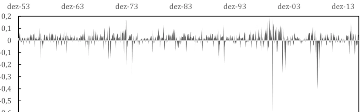
Figure 1: Momentum returns (MoM_Reg) from April 1953 to December 2016

... 13

(8)

List of Tables

Table 1: Predictive power of Market State (MKT) and Market Volatility (Vol).

... 19 Table 2: Predictive power of Market State (MKT), Market Volatility (Vol), Dividend Yield on the CRSP value-weighted index (DIV), Yield Spread between Baa-rated bonds and Aaa-rated bonds (DEF), Yield Spread between ten-year Treasury bonds and three-month Treasury bills (TERM) and Yield on a T-bill with three month to maturity (YLD). ... 21

Table 3: Comparison between predictive power of Market State (MKT) and

Market Volatility (Vol) using the original variables (A1) and using the frequency-components of the variables (WAV_A1_D4) ... 23

Table 4: Comparison between predictive power of Market State (MKT),

Market Volatility (Vol), Dividend Yield on the CRSP value-weighted index (DIV), Yield Spread between Baa-rated bonds and Aaa-rated bonds (DEF), Yield Spread between ten-year Treasury bonds and three-month Treasury bills (TERM) and Yield on a T-bill with three month to maturity (YLD) using the original variables (B1, B2 and B3) and using the frequency-components of the variables (WAV_B1_D4, WAV_B2_D4 and WAV_B3_D4) ... 24

(9)

Introduction

Momentum investing is a trading strategy that aims to capitalize on the confirmation of recent trends of asset returns. Considering a particular backward time window, traders take a long position (i.e. buy) in assets that have posted positive returns during that time window and/or take a short position (i.e. sell) on assets that posted negative returns during the same time window. That is, the momentum strategy implies buying past winners and/or selling past losers. Momentum is considered an anomaly in financial markets which finance theory struggles to explain. Jegadeesh and Titman (1993) found that when stocks are ranked on the basis of their past returns, then past winners outperform the past loser in the medium-term period. They document that momentum strategies implemented in the U.S. equity market from 1965 to 1989 generated a positive profit of about one percent per month over 3 to 12 month holding periods. Rouwenhorst (1998), extend the work of Jegadeesh and Titman (1993) to a non-U.S. equity market approach showing that an internationally diversified portfolio which invests in medium-term winners and sells past medium-term losers earns around one percent per month. More recently, Asness et al. (2013), provided evidence on the return premia to value and momentum strategies globally across different asset classes. The momentum strategies in equity markets have historically delivered high Sharpe ratios. However, returns of these strategies also display substantial time-variation and are exposed to rare but severe drawdowns. Daniel and Moskowitz (2016) showed that momentum trading strategies carry a significant downside risk and potential momentum crashes. They document that momentum returns are negatively skewed, and the negative returns can be pronounced and persistent.

(10)

10

The extensive literature on momentum has been essentially focused on what causes momentum, the description of momentum across industry sectors and countries and on its risk management. Cooper, Gutierrez, and Hameed (2004, hereafter CGH) tested the theory that overreaction is the source of short-run momentum and the long run reversal in the cross section of stock returns finding that the extent to which investors are affected by psychological biases that causes momentum depends on the market state. Antoniou, Doukas and Subrahmanyam (2013) confirm the results of CGH and show that sentiment has incremental power to explain momentum-induced profits after accounting for market returns. Similarly, Hillert et al. (2014) showed that media coverage can influence investors’ biases supporting an over-reaction based explanation of momentum effect suggested by CGH while Hvidkjaer (2006) suggested that momentum could partly be driven by the underreaction of small traders. Also there is recent evidence that momentum is somehow driven by changes in firm fundamentals (Novy-Marx, 2015). Most of the literature focuses on the relative performance of securities in the cross-section, finding that securities that recently outperformed their peers over the past three to 12 months continue to outperform their peers on average over the next month. Alternatively, Moskowitz, Ooi and Pedersen (2012) rather than focus on the relative returns of securities in the cross-section, document the time series momentum, which focuses purely on a security’s own past return. Avramov, Cheng, and Hameed (2013) test the effects of time-varying liquidity showing that momentum profits are markedly larger in liquid market states. On the other hand, Da et al. (2014), show that the momentum premium is stronger in stocks experiencing frequent but small price changes that are less likely to attract attention. My work is most closely related to a recent branch of the literature focused on the predictability of momentum returns. Huang (2015) proposes a momentum gap variable (i.e. the formation period return difference between past winners and losers) that is negatively correlated with momentum

(11)

11

profits after controlling for existing predictors. Barroso and Santa-Clara (2015) find that the risk of momentum is highly variable over time and predictable and managing that risk virtually eliminates crashes and approximately doubles the Sharpe ratio of the momentum strategy. Jacobs et al. (2015) suggest that the momentum premium can be explained by the expected skewness of momentum.

In the same line of the latter subset of the literature is the work developed by Wang & Xu (2015; hereafter WX) who show that market volatility can predict momentum returns, which is the starting point of my investigation. They found that the volatility of market returns has indeed significant and robust power to forecast momentum payoffs, particularly in negative market states. They also show that the predictive power of market volatility persists after controlling for market states and business cycle variables.

My focus is to re-evaluate momentum returns predictability introducing a frequency decomposition approach of the predictors rather than using the original predictors. In this study, I start by analyzing the results obtained by WX. Then, I examine the momentum predictability after applying a wavelet transformation to WX variables comparing the results of the original predictive regressions with the ones obtained in a frequency domain approach. Motivated by the work developed by Faria and Verona (2018), I examine whether using wavelet methods to decompose the predictors in several frequencies rather than using the original variables, generates an improvement in momentum returns predictability. Being an extension of the Fourier analysis, wavelet analysis allow one to take into account both the time and the frequency domains. Wavelet analysis enables the researcher to explore how variables are related at different frequencies and how such relationship has evolved over time. Crowley (2007), Aguiar-Conraria and Soares (2014) and Rua (2012), among others, provided reviews on the usefulness of wavelet methods in economics and finance and its application. While the extensive literature on momentum exploits the

(12)

cross-12

section and/or the time-series dynamics of momentum returns, this work aims to bring an innovative approach to the existing theories. WX provide a straightforward analysis on how market returns volatility can predict momentum returns. I compare the predictive power of a set of predictors documented by WX with the predictive power of the same variables after being decomposed with wavelet methods. I apply the maximal overlap discrete wavelet transform (MODWT) multiresolution analysis (MRA) which allows the decomposition of a given time series into different time series (i.e. its frequency components). I provide evidence that decomposing the predictors in their frequency components yields statistically significant gains in terms of robustness. This research aims to challenge existing literature proposing a new wavelet-based method to study momentum returns predictability. The rest of this dissertation is structured as follows. Section 1 presents the data and the methodology. In section 2 I provide the results of the regressions. Section 3 concludes.

(13)

1. Data and Methodology

1.1 Data

I re-evaluate the momentum returns predictability power of the set of predictors analyzed in WX. The novelty of our analysis is that we consider different frequencies of this set of predictors.

In the first regression (A1) the sample period is from January 1930 to December 2016. In the following three regressions (B1, B2 and B3) the sample covers April 1953 to December 2016 (the period we have business cycle data).1_{The dependent}

variable (Yt) is the monthly momentum returns from Ken French data library. Stocks are sorted into deciles based on their past returns from month t-12 to month t-2 forming ten equal-weighted portfolios. The holding month is t. The portfolio with the highest (lowest) past return is the winner (loser) portfolio. The momentum return in month t is the return of the winner portfolio minus the return of the loser portfolio.

1_{WX use January 1930 to December 2009 as sample period for the first regression and April 1953 to}

December 2009 for the following three regressions.

-0,6 -0,5 -0,4 -0,3 -0,2 -0,1 0 0,1 0,2

dez-53 dez-63 dez-73 dez-83 dez-93 dez-03 dez-13

Figure 1: Momentum returns (Mom_Reg) from April 1953 to December 2016. Regular

construction of momentum. Stocks are sorted into deciles based on their past returns from month t-12 to month t-2 forming ten equal-weighted portfolios. The holding month is t. The portfolio with the highest (lowest) past return is the winner (loser) portfolio. The momentum return in month t is the return of the winner portfolio minus the return of the loser portfolio.

(14)

14

1.2. Predictors used in the analysis

MKT: Market State - computed as the average of the past three years monthly returns on the value-weighted CRSP index from month t-36 to month t-1. Data is obtained from the Goyal and Welch dataset.

Vol: Market Volatility - calculated as the standard deviation of the daily returns on the CRSP index from month t-12 to month t-1.

DIV: Dividend Yield - obtained from the difference between the log of dividends and the log of lagged prices from the CRSP value-weighted index. (This and the next three variables are obtained from the Goyal and Welch dataset) DEF: Corporate Yield Spread - is the lagged yield spread between Baa and Aaa corporate bond yields measured at the end of month t-1.

TERM: Term Yield Spread - is the lagged yield spread between ten-year treasury bonds and three month treasury bills measured at the end of month t-1. YLD: Yield - is the yield on a T-Bill with three months to maturity measured at the end of month t-1.

1.3. The four regressions

I start by replicating Table 2 of WX where all the regressions are of the form: Y_𝑡 = c + bX_𝑡−1 + e_𝑡

I run four pairs of regressions:

Regression A1:

(15)

15 Regression B1: 𝑀𝑜𝑀_𝑅𝑒𝑔𝑡= 𝛽0+ 𝛽1𝑀𝐾𝑇𝑡−1+ 𝛽2𝑉𝑜𝑙𝑡−1+ 𝛽3𝐷𝐼𝑉𝑡−1+ 𝛽4𝐷𝐸𝐹𝑡−1 + 𝛽₅𝑇𝐸𝑅𝑀_𝑡−1+ 𝛽₆𝑌𝐿𝐷_𝑡−1+ ℇ_𝑡 Regression B2: 𝑀𝑜𝑀_𝑆𝑏𝑡= 𝛽0+ 𝛽1𝑀𝐾𝑇𝑡−1+ 𝛽2𝑉𝑜𝑙𝑡−1+ 𝛽3𝐷𝐼𝑉𝑡−1+ 𝛽4𝐷𝐸𝐹𝑡−1 + 𝛽5𝑇𝐸𝑅𝑀𝑡−1+ 𝛽6𝑌𝐿𝐷𝑡−1+ ℇ𝑡 Regression B3: 𝑀𝑜𝑀_𝐵𝑖𝑔_𝑡 = 𝛽₀+ 𝛽₁𝑀𝐾𝑇_𝑡−1+ 𝛽₂𝑉𝑜𝑙_𝑡−1+ 𝛽₃𝐷𝐼𝑉_𝑡−1+ 𝛽₄𝐷𝐸𝐹_𝑡−1 + 𝛽5𝑇𝐸𝑅𝑀𝑡−1+ 𝛽6𝑌𝐿𝐷𝑡−1+ ℇ𝑡

In each pair I first use the original variables of WX and then I run the same regression with the frequency decomposed variables. In Table 1 I start by regressing momentum returns (regular momentum construction) on two explanatory variables – Market State (MKT) and Market Volatility (Vol). Then, I add the four business cycle variables (DIV, DEF, TERM, YLD), with results reported in Table 2. The three regressions of Table 2 only differ on the way the

momentum return (the dependent variable) is constructed. In regression B1, the momentum variable is constructed on a regular way. The portfolio with the highest (lowest) past monthly return is the winner (loser) portfolio. MoM_Reg is the month return difference between the winner and loser portfolios. In regression B2, momentum returns correspond to the profit of a size-balanced momentum portfolio. Ken French database provides the returns of six value-weighted portfolios formed on size and past returns, denoted as Small High, Small Medium, Small Low, Big High, Big Medium and Big Low. MoM_Sb is the average return on the two high prior return portfolios (Small High and Big High) minus the average return on the two low prior return portfolios (Small Low and Big Low). Finally, in regression B3, momentum payoff if computed using large

(16)

16

stocks only. MoM_Big corresponds to the return difference between equally-weighted Big High and Big Low portfolios.

1.4. Wavelet Transform

Spectral analysis and Fourier transforms have been, for a long time, the most common frequency domain methods used. The Fourier transform is a powerful tool for data analysis. However, it does not capture well abrupt changes efficiently, that is, it does not work properly with structural brakes in the variables under analysis. The reason for this is that the Fourier transform represents data as a sum of sinusoidal waves, which are not localized in time or space. These sinusoidal waves oscillate indefinitely. Conversely, frequency domain wavelets-based methods enable to analyze data series that have abrupt changes. A wavelet is an oscillation in the form of a wave with zero-mean and that decays rapidly. Unlike sinusoids, which extend to infinity, a wavelet exists for a finite duration. Wavelets come in different sizes and shapes. . The choice of the concrete wavelet filter (e.g. Haar, Daubechies, Coiflets or Symlets) is basically connected to two fundamental properties of each wavelet transform: scaling and shifting. Scaling refers to the process of stretching or shrinking the wave in time. The scale factor is inversely proportional to frequency. For example, scaling a sine wave by 2 results in reducing its original frequency by half. For a wavelet, there is a reciprocal correlation between scale and frequency with a constant of proportionality. This constant of proportionality is called the "center frequency" of the wavelet. This is because, unlike the sinewave, the wavelet works in a time-frequency domain. A larger scale factor results in a stretched wavelet, which corresponds to a lower frequency. A smaller scale factor generates a shrunken wavelet, which corresponds to a high frequency. A stretched wavelet helps in capturing the slowly varying changes in a signal while a compressed wavelet

(17)

17

helps in capturing abrupt changes. On the other hand, shifting a wavelet simply means deferring or advancing the beginning of the wavelet along the length of the signal. A wavelet is shifted to align with the feature we are looking for in a signal.

The decomposition process of a given time series into different time series is known as multiresolution analysis (MRA). By applying a maximal overlap discrete wavelet transform multiresolution analysis (MODWT MRA), a time series yt is decomposed as:

𝑦_𝑡 = 𝑦(𝐷₁)_𝑡+ . . . + 𝑦(𝐷_𝐽)_𝑡 + 𝑦(𝑆_𝐽)_𝑡

where the 𝑦(𝐷₁)_𝑡= 1,2, … , 𝐽 are the wavelet details and 𝑦(𝑆𝐽)𝑡 is the wavelet smooth component. The original time series is therefore decomposed into orthogonal components (𝑦(𝐷1)𝑡 to 𝑦(𝐷𝐽)𝑡 and 𝑦(𝑆𝐽)𝑡), each defined in the time domain and representing the fluctuation of the original time series in a specific frequency band. For small j, the J wavelet details represent the higher frequency characteristics of the time series (i.e. its short-term dynamics) and, as j increases, the j wavelet details represent lower frequencies movements of the series. The wavelet smooth captures the lowest frequency dynamics (i.e. its long-term behavior or trend).

In this dissertation, I replicate four regressions on momentum predictability from WX but instead of using the original variables I use the frequency components 𝐷1, 𝐷2,..., 𝐷𝐽 for each of the variables. The number of frequency bands (J) used in the wavelet analysis to decompose the time series depends on the number of observations under analysis.2_{In the three wavelet regressions of}

Table 4, given the 765 observations used, I apply a J=8 level MRA so that the

2_{In Table 4, N = 765 is the number of observations in the in-sample period, so J is such that 𝐽 ≤ 𝑙𝑜𝑔}₂𝑁 ≅

(18)

18

wavelet decomposition delivers nine orthogonal crystals: eight wavelet details (𝑦(𝐷1)𝑡 to 𝑦(𝐷8)𝑡) and the wavelet smooth (𝑦(𝑆8)𝑡). As I use monthly data, the first detail level 𝑦(𝐷1)𝑡 captures oscillations between 2 and 4 months, while detail levels 𝑦(𝐷2)𝑡 , 𝑦(𝐷3)𝑡 , 𝑦(𝐷4)𝑡 , 𝑦(𝐷5)𝑡 , 𝑦(𝐷6)𝑡 , 𝑦(𝐷7)𝑡 , 𝑦(𝐷8)𝑡 , capture oscillations with a period of 4-8, 8-16, 16-32, 32-64, 64-128, 128-256, 256-512 months, respectively. Finally, the smooth component y (S6)t captures oscillations with a period longer than 512 months (approximately 42.6 years). In the wavelet regression of Table 3, since I use a longer sample (1044 observations), I apply a J=10 level MRA.

2. Results

In this section I describe the results obtained. In subsection 2.1 I present the results of momentum returns predictability using the original time series of the predictors under analysis. In section 2.2 I provide the results of the application of the wavelet filtering methods and the comparison with the ones obtained in the time series analysis in section 2.1. For the sake of consistency, the interpretation

0 0,005 0,01 0,015 0,02 0,025 0,03 0,035

dez-30 dez-40 dez-50 dez-60 dez-70 dez-80 dez-90 dez-00 dez-10

Figure 2: Market Volatility (Vol) from January 1930 to December 2016. Calculated as the

(19)

19

of the coefficients across all the paper is done based on a two-sided t-student distribution with for the 90%, 95% and 99%confidence intervals.

2.1. Momentum returns predictability with original

predictors

Regression A1:

𝑀𝑜𝑀_𝑅𝑒𝑔_𝑡 = 𝛽₀+ 𝛽₁𝑀𝐾𝑇_𝑡−1+ 𝛽₂𝑉𝑜𝑙_𝑡−1+ ℇ_𝑡

In all the tables of results reported in this dissertation I provide both the coefficient and the t-statistics of the variables used. The latter is the measure I use to assess the statistical significance of the variables. T-statistic allows one to test the null hypothesis that the corresponding coefficient is zero against the alternative that it is different from zero, given the other predictors in the model. It is computed by dividing the statistical estimate of the coefficient by the estimated standard error. Thus, to establish the statistical significance of the variable I compare the obtained t-statistic with the critical values of a t distribution for the three most common confidence intervals – 90%, 95% and 99%.

Variables Coefficients

(robust t-statistics)

(Momentum Returns) MoM_Reg (A1)

MKT 0,82 (1,36) Vol -1,78** (-2,57) R-Squared (percentage) 3,47

Table 1: Predictive power of Market State (MKT) and Market Volatility (Vol).

Predictors are measured at the end of month t-1. The dependent variable is measured at month t. I omit the constant term coefficient for brevity. The sample period is from January 1930 to December 2016. 1044 observations were used.

(20)

20

In the tables, the coefficients are identified with one, two or three asterisks (*) for variables that are statistically significant with 90%, 95% and 99% confidence, respectively.3_{Finally, I provide the coefficient of determination for all regressions}

(R-squared) which allows to assess variations in their predictive power of momentum returns when moving from the time-domain to the frequency domain.

Table 1 presents the results of the predictive regression A1, which considers

the Market State (MKT) and Market Volatility (Vol) as predictors of Momentum Returns (MoM_Reg). Reported results show that Market State (MKT) is not a statistically significant predictor of the momentum returns whereas Market Volatility (Vol) is a significant predictor. This set of results contrasts with those reported in WX with respect to the predictor MKT. That difference arises from the fact that WX use a shorter sample period and also due to some corrections in the data that occurred since they finished their work.4

Regression B1: 𝑀𝑜𝑀_𝑅𝑒𝑔_𝑡= 𝛽₀+ 𝛽₁𝑀𝐾𝑇_𝑡−1+ 𝛽₂𝑉𝑜𝑙_𝑡−1+ 𝛽₃𝐷𝐼𝑉_𝑡−1+ 𝛽₄𝐷𝐸𝐹_𝑡−1 + 𝛽5𝑇𝐸𝑅𝑀𝑡−1+ 𝛽6𝑌𝐿𝐷𝑡−1+ ℇ𝑡 Regression B2: 𝑀𝑜𝑀_𝑆𝑏_𝑡= 𝛽₀+ 𝛽₁𝑀𝐾𝑇_𝑡−1+ 𝛽₂𝑉𝑜𝑙_𝑡−1+ 𝛽₃𝐷𝐼𝑉_𝑡−1+ 𝛽₄𝐷𝐸𝐹_𝑡−1 + 𝛽5𝑇𝐸𝑅𝑀𝑡−1+ 𝛽6𝑌𝐿𝐷𝑡−1+ ℇ𝑡 Regression B3: 𝑀𝑜𝑀_𝐵𝑖𝑔𝑡 = 𝛽0+ 𝛽1𝑀𝐾𝑇𝑡−1+ 𝛽2𝑉𝑜𝑙𝑡−1+ 𝛽3𝐷𝐼𝑉𝑡−1+ 𝛽4𝐷𝐸𝐹𝑡−1 + 𝛽₅𝑇𝐸𝑅𝑀_𝑡−1+ 𝛽₆𝑌𝐿𝐷_𝑡−1+ ℇ_𝑡

3_{The critical values for the two sided t-distribution used are 1.64, 1.96, and 2.58 for 90%, 95% and 99%}

confidence interval, respectively.

4_{In unreported results, WX’s sample period was used. Goyal and Welch database is updated and corrected}

(21)

21

Table 2 presents the results of the predictive regressions B1, B2 and B3. Versus the regression A1, four additional business cycle variables were considered – DIV, DEF, TERM, and YLD. The difference between those three regressions is exclusively related with the dependent variable. Momentum returns are firstly computed in a regular way, then from a size-balanced portfolio and finally using large stocks only for regressions B1, B2 and B3 respectively. Contrasting with the findings of WX, the results from Table 2 show that in most

of the cases under analysis these business cycle related variables don’t have significant predictive power of the time-variation in momentum profits. Regarding regression B1 there is evidence that DIV is statistically irrelevant, while DEF and TERM are only significant in the 90% confidence interval. In

Variables Coefficients

(robust t-statistics)

(Momentum Returns) MoM_Reg (B1) MoM_Sb (B2) MoM_Big (B3)

MKT 0,50 (1,47) 0,30 (1,24) 0,23 (0,87) Vol -2,20** (-2,21) -1,24** (-1,96) -1,40** (-2,14) DIV 0,02 (1,20) 0,82 (1,36) 0,00 (-0,19) DEF -1,70* (-1,71) 0,00 (0,01) 0,70 (-0,98) TERM 0,37* (1,72) 0,31** (2,02) 0,22 (1,44) YLD 0,29*** (2,60) 0,15* (1,74) 0,09 (1,01) R-Squared (percentage) 6,22 4,34 3,30

Table 2: Predictive power of Market State (MKT), Market Volatility (Vol), Dividend Yield on the

CRSP value-weighted index (DIV), Yield Spread between Baa-rated bonds and Aaa-rated bonds (DEF), Yield Spread between ten-year Treasury bonds and three-month Treasury bills (TERM) and Yield on a T-bill with three month to maturity (YLD). Three different measures for momentum returns are used for B1. Predictors are measured at the end of month t-1. The dependent variable is measured at month t. I omit the constant term coefficient for brevity. The sample period is from April 1953 to December 2016. 765 observations were used.

(22)

22

regression B2, TERM has a robust t-statistic above 1,96 (i.e. 95% confidence interval) in absolute value while YLD is only significant with a 90% confidence interval. For regression B3 the predictive power of the business cycle variables is always statistically insignificant, even considering the narrowest confidence interval, with t-statistics ranging from -0,98 to 1,44. Another interesting finding is that MKT is also statistically insignificant across all three regressions. The state of the market in the previous three years seems to be insignificant to predict time-variations in momentum returns independently of how they are measured. In contrast, Market Volatility (Vol) remains significant throughout all cases showing robust predictive power in the presence of market state and business cycles variables even when momentum profits are measured from size-balanced or with large stocks portfolios.

2.2. Regressions with frequency-decomposed predictors

After analyzing the results of the four regressions above, in this subsection I examine whether replacing the original variables by their frequency components delivers improved predictability. In Table 3 and Table 4 I present the t-statistic and the R-squared of the same regressions introduced above (A1, B1, B2, B3 and B4) comparing with the results obtained when applying the frequency decomposition techniques explained in section 1.3 to the same variables. For brevity, in both tables I present only the wavelet regressions that were run using reflection as boundary and haar as wavelet filter. The purpose was to pick the combination of wavelet filter and boundary that delivered the best result out of the twenty combinations tested.5

5_{For robustness checks all regressions were run for two boundaries – reflection and periodic – combined}

(23)

23

Variables _{Robust t-statistics}

(Regression) A1 WAV_A1_D4

MKT 1,35 1,02

Vol -2,57** -3,60***

R-Squared

(percentage) 3,47 3,78

Table 3: Comparison between predictive power of Market State (MKT) and Market Volatility

(Vol) using the original variables (A1) and using the frequency-components of the variables (WAV_A1_D4). In regression WAV_A1_D4 the boundary used is reflection and the wavelet filter used is haar. The detail level presented is D4. Predictors are measured at the end of month t-1. The dependent variable is measured at month t. I omit the constant term coefficient for brevity. The sample period is from January 1930 to December 2016. 1044 observations were used.

Results in Table 3 are in line with those reported in Table 1. Analyzing the regression in the frequency domain, the detail level D4 was the one delivering the strongest results. When replacing the original variables by their frequency component of level 4, capturing oscillations with a period from 16 to 32 months, the statistical significance of both variables remains the same. Market state (MKT) continuous to be irrelevant to predict momentum returns presenting a weaker t-statistic in absolute value in the frequency domain analysis. In contrast, the predictive power of Market Volatility (Vol) increases with a robust t-statistic of 3,60 (in absolute value), being significant at a wider confidence interval. Considering the regression as a whole, the results presented in Table 3 suggest a slight improvement in the coefficient of determination when moving from the original variables to the frequency domain. R-squared increases from 3,47 to 3,78 (in percentage terms).

(24)

Variables _{Robust t-statistics}

(Regression) B1 WAV_B1_D4 B2 WAV_B2_D4 B3 WAV_B3_D4

MKT 1,47 1,90* 1,24 1,40 0,87 1,46 Vol -2,21** -3,52*** -1,96** -3,40*** -2,14** -3,79*** DIV 1,20 -0,07 0,01 0,28 -0,19 0,34 DEF -1,71* -1,24 -1,33 -0,87 -0,98 -0,83 TERM 1,72* 1,97** 2,02** 1,64* 1,44 1,55 YLD 2,60*** 2,17** 1,74* 0,70 1,01 0,63 R-Squared (percentage) 6,22 7,70 4,34 5,80 3,30 5,57

Table 4: Comparison between predictive power of Market State (MKT), Market Volatility (Vol), Dividend Yield on the CRSP value-weighted index (DIV),

Yield Spread between Baa-rated bonds and Aaa-rated bonds (DEF), Yield Spread between ten-year Treasury bonds and three-month Treasury bills (TERM) and Yield on a T-bill with three month to maturity (YLD) using the original variables (B1, B2 and B3) and using the frequency-components of the variables (WAV_B1_D4, WAV_B2_D4 and WAV_B3_D4). Three different measures for momentum returns are used for B1, B2 and B3 (WAV_B1_D4, WAV_B2_D4 and WAV_B3_D4, respectively). In all wavelet regressions (WAV_B1_D4, WAV_B2_D4 and WAV_B3_D4) the boundary used is reflection and the wavelet filter used is haar. The detail level presented is D4. Predictors are measured at the end of month t-1. The dependent variable is measured at month t. I omit the constant term coefficient for brevity. The sample period is from April 1953 to December 2016. 765 observations were used.

(25)

Table 4 presents the comparison between time series and the frequency

domain analysis of the predictive power of Market State (MKT) and Market Volatility (Vol) jointly with the four business cycle variables added (DIV, DEF, TERM, YLD). The main conclusion is that the statistical significance of the variables is practically the same when selecting their best frequency for predictability purposes (again the D4) instead of using its original time series. An important exception is TERM. Its D4 detail level is a statistically significant predictor of momentum returns when the latter is constructed on a regular way (from 1,72 to 1,97). In contrast, when momentum profits are measured from a size balanced portfolio, the predictive power of TERM loses its statistical significance (2,02 to 1,64). On the other hand, Market State (MKT), that had shown to be irrelevant until here, turns out to be a reasonable predictor of momentum returns but only when they are computed in a regular way and at a 90% confidence interval. Finally, as in Table 3, Market Volatility (Vol) confirms its robust predictive power of momentum profits. Its t-statistic increases for all the three wavelet-based regressions (in absolute value). Overall, there is an increase in the estimated R-squared across all three regressions, with growths ranging from 1,46 percentage points (B2 to WAV_B2_D4) to 2,27 percentage points (B3 to WAV_B3_D4).

(26)

26

3. Conclusion

Wang and Xu (2015) showed that the time-variation of momentum returns can be exploited in much more detail. Concretely, they documented the potential of Market Volatility in predicting momentum profits. In this study, I started by establishing those findings by extending Wang and Xu (2015) sample period analysis. Additionally, I further extend the scope of the analysis to the frequency domain bringing an innovative perspective to the existing momentum related literature. I find that decomposing the original time series of the predictors delivers statistically significant gains in terms of robustness for some predictors. By decomposing the original time series in its different frequencies and then choosing the proper detail level, the quality of the regression improves. I provide evidence that the coefficient of determination (R-squared) increases for all the four regressions when the original predictors are replaced by their frequency components. This dissertation aims to challenge existing literature on momentum returns predictability, proposing a wavelet-based method. On the other hand, it is expected to be useful for forecasting other financial or macroeconomic variables (such as volatility or inflation). It would be interesting to re-evaluate the results obtained by Barroso and Santa-Clara (2015) on the highly time-varying risk of momentum and its predictability under the frequency domain by using wavelet methods since they enable to analyze data series that have abrupt changes.

(27)

27

Bibliography

Aguiar-Conraria, L., & Soares, M. J. 2014. The continuous wavelet transform: Moving beyond uni- and bivariate analysis. Journal of Economic Surveys, 28(2): 344–375.

Antoniou, C., Doukas, J. A., & Subrahmanyam, A. 2013. Cognitive dissonance, sentiment, and momentum. Journal of Financial and Quantitative Analysis, 48(1): 245–275.

Asness, C. S., Moskowitz, T. J., & Pedersen, L. H. 2013. Value and Momentum Everywhere. Journal of Finance, 68(3): 929–985.

Avramov, D., Cheng, S., & Hameed, A. 2016. Time-varying liquidity and momentum profits. Journal of Financial and Quantitative Analysis, 51(6): 1897– 1923.

Baker, M., & Wurgler, J. 2006. Investor sentiment and the cross-section of stock returns. Journal of Finance, 61(4): 1645–1680.

Barroso, P., & Santa-Clara, P. 2015. Momentum has its moments. Journal of Financial Economics, 116(1): 111–120.

Barroso, P., & Santa-Clara, P. 2012. Managing the Risk of Momentum. SSRN Electronic Journal. https://doi.org/10.2139/ssrn.2041429.

Berghorn, W. 2015. Trend momentum. Quantitative Finance, 15(2): 261–284. Chaovalit, P., Gangopadhyay, A., Karabatis, G., & Chen, Z. 2011. Discrete wavelet transform-based time series analysis and mining. ACM Computing Surveys, 43(2): 1–37.

Chordia, T., & Shivakumar, L. 2002. Momentum, business cycle, and time-varying expected returns. Journal of Finance, 57(2): 985–1019.

Cooper, M. J., Gutierrez, R. C., & Hameed, A. 2004. Market states and momentum. Journal of Finance.

(28)

28

Crowley, P. M. 2007. A guide to wavelets for economists. Journal of Economic Surveys, 21(2): 207–267.

Da, Z., Gurun, U. G., & Warachka, M. 2014. Frog in the pan: Continuous information and momentum. Review of Financial Studies, 27(7): 2171–2218. Daniel, K., & Moskowitz, T. J. 2016. Momentum crashes. Journal of Financial Economics, 122(2): 221–247.

Faria, G., & Verona, F. 2018. Forecasting stock market returns by summing the frequency-decomposed parts. Journal of Empirical Finance, 45: 228–242.

Han, Y., & Zhou, G. 2014. Taming Momentum Crashes: A Simple Stop-Loss Strategy. SSRN Electronic Journal. https://doi.org/10.2139/ssrn.2407199.

Hillert, A., Jacobs, H., & Müller, S. 2014. Media makes momentum. Review of Financial Studies.

Huang, S. 2013. The Momentum Gap and Return Predictability. Unpublished Working Paper.

Hung, S. Y. K., & Glascock, J. L. 2008. Momentum profitability and market trend: Evidence from REITs. Journal of Real Estate Finance and Economics, 37(1): 51– 69.

Hvidkjaer, S. 2006. A trade-based analysis of momentum. Review of Financial Studies, 19(2): 457–491.

Jacobs, H., Regele, T., & Weber, M. 2015. Expected Skewness and Momentum. CEPR Discussion Papers 10601, C.E.P.R. Discussion Papers.

Jegadeesh, N., & Titman, S. 2011. Momentum. Annual Review of Financial Economics, 3(1): 493–509.

Min, B. K., & Kim, T. S. 2016. Momentum and downside risk. Journal of Banking and Finance, 72: S104–S118.

Moskowitz, T. J., Ooi, Y. H., & Pedersen, L. H. 2012. Time series momentum. Journal of Financial Economics, 104(2): 228–250.

(29)

29

Novy-Marx, R. 2015. Fundamentally, momentum is fundamental momentum. NBER Working Paper Series, 1–45.

Pástor, Ľ., & Stambaugh, R. F. 2003. Liquidity Risk and Expected Stock Returns. Journal of Political Economy, 111(3): 642–685.

Rouwenhorst, K. G. 1998. International momentum strategies. Journal of Finance, 53(1): 267–284.

Rua, A. 2012. Wavelets in economics. Economic Bulletin and Financial Stability Report Articles, Banco de Portugal.

Walden, A. T. 2001. Wavelet Analysis of Discrete Time Series. European Congress of Mathematics, 202(1): 627–641.

Wang, K. Q., & Xu, J. 2015. Market volatility and momentum. Journal of Empirical Finance, 30: 79–91.

Welch, I., & Goyal, A. 2008. A comprehensive look at the empirical performance of equity premium prediction. Review of Financial Studies, 21(4): 1455–1508.

Momentum predictability in the frequency domain