Equity valuation of Distribuidora Internacional de Alimentación (DIA)

(1)

Equity Valuation of

Distribuidora Internacional

de Alimentación (DIA)

Francisco Lemos

Dissertation written under the supervision of Professor

José Tudela Martins

Dissertation submitted in partial fulfilment of requirements for the MSc in

(2)

Sumário Executivo

Nome do estudante: Francisco Lemos para o Msc in Finance da Católica Lisbon School of Business & Economics

Título: Equity Valuation of Distribuidora Internacional de Alimentación (DIA)

O objetivo desta dissertação é determinar o valor justo dos capitais próprios da Distribuidora Internacional de Alimentación. O setor do retalho de produtos alimentares foi investigado detalhadamente, bem como a empresa e o seu modelo de negócio. A Revisão Literária apresenta uma discussão de diferentes abordagens teóricas de avaliação de empresas e considera que o método dos fluxos de caixa descontados com soma das partes e uma avaliação por múltiplos são os métodos mais apropriados para avaliar a empresa. Com esta avaliação, é razoável assumir que as ações da empresa estão cotadas abaixo do seu valor intrínseco, €4,79, o que representa um potencial de valorização de 11,3% e, assim, uma recomendação de “compra”. Esta avaliação é também comparada com um equity research do BPI, focando-se nas metodologias e pressupostos usados em ambos os trabalhos.

(3)

Abstract

Student name: Francisco Lemos for the MSc in Finance in Católica Lisbon School of Business & Economics

Title: Equity Valuation of Distribuidora Internacional de Alimentación (DIA)

The aim of this dissertation is to determine the fair value of Distribuidora Internacional de Alimentación equity. The retail food sector was research in detail, as well as the company and its business model. The Literature Review presents a discussion of different valuation theoretical approaches and it considers that a sum of the parts discounted cash flow valuation and a multiple valuation are the most accurate methods to evaluate the company. With this evaluation, it is reasonable to assume that the company’s shares are trading below their intrinsic value, €4,79, which represents a 11,3% potential appreciation and, thus, a “buying” recommendation. This valuation is also compared with an equity research from BPI, focusing on the methodologies and assumptions used on both works.

(4)

Acknowledgments

This dissertation is the final step of the MSc in Finance of Católica Lisbon School of Business & Economics and it represents two years of hard work, interesting challenges and personal enrichment. I am sure that this journey will provide an invaluable milestone in my personal development and professional career.

I would like to express my gratitude to Professor José Carlos Tudela, for his availability and useful guidance throughout this process; to my colleagues, for all the fruitful insights and discussions; and to my Family and friends for all the demonstrations of love and support.

(5)

List of figures

Figure 2.1 - Equity risk premium formula with country risk premium ... 19

Figure 2.2 – Types of multiples ... 23

Figure 3.1 - Sales in Spain grocery retailers by channel, in Million USD (source: Euromonitor) ... 26

Figure 3.2 - Spain grocery retailers market share 2017 (source: Statista) ... 26

Figure 3.3 - Portugal grocery retailers market share 2017 (source: BPI Equity Research) ... 27

Figure 3.4 - CAGR in grocery retailers in Portugal by channel, 2013-18f (source: Planet Retail) ... 27

Figure 3.5 - Market share of private labels in Portugal, 2009-13 (source: Nielsen) ... 28

Figure 3.6 - Spain historical and forecasted real GDP growth and inflation (source: IMF) .... 30

Figure 3.7 - Unemployment rate and retail sales growth in Spain (source: National Statistics Institue of Spain and Bloomberg) ... 31

Figure 3.8 – Portugal historical and forecasted real GDP growth and inflation (source: IMF)31 Figure 3.9 - Unemployment rate and retail sales growth in Spain (source: National Statistics Institute of Portugal and Bloomberg) ... 32

Figure 3.10 - Argentina historical and forecasted real GDP growth and inflation (source: IMF) ... 32

Figure 3.11 - Brazil historical and forecasted real GDP growth and inflation (source: IMF) . 33 Figure 3.12 - Historical and estimated FX rates for Argentina and Brazil (source: Bloomberg) ... 33

Figure 4.1 - DIA private labels by market in 2016 ... 36

Figure 4.2 - DIA's neighborhood store network format ... 36

Figure 4.3 - DIA's larger store network formats ... 37

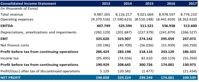
Figure 4.4 - Historical consolidated income statement (2013 - 2017) ... 39

Figure 4.5 - Iberia historical operating indicators (2013 - 2017) ... 39

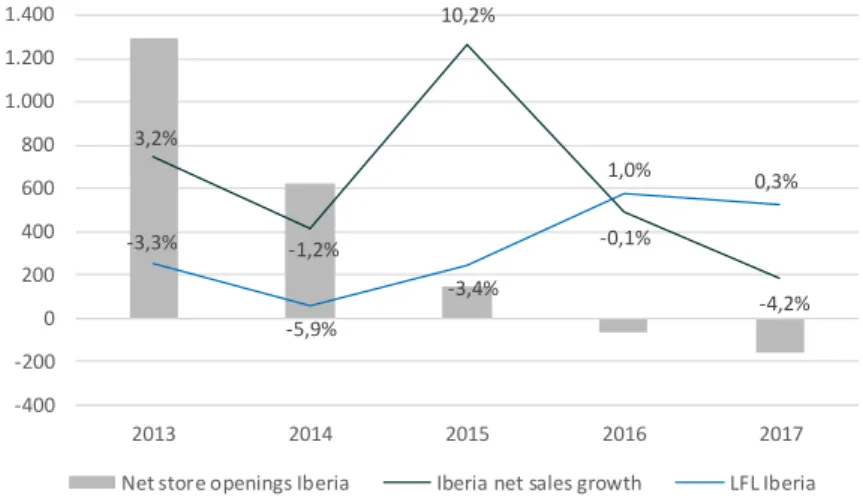
Figure 4.6 - Historical sales growth in Iberia (2013 - 2017) ... 40

Figure 4.7 - Emerging Markets historical operating indicators (2013 – 2017) ... 41

Figure 4.8 - Emerging Markets historical sales growth (2013 - 2017) ... 41

Figure 4.9 - Historical operating costs as % of total operating costs (2013 – 2017) ... 42

Figure 5.1 - Estimated LFL growth in Iberia ... 44

Figure 5.2 - Estimated net store openings in Iberia ... 44

(9)

Figure 5.4 - Portugal forecasted revenues (in million Euros) ... 45

Figure 5.5 - Estimated LFL growth in Emerging Markets ... 45

Figure 5.6 - Estimated net store openings in Emerging Markets ... 46

Figure 5.7 - Estimated FX rates ... 47

Figure 5.8 - Argentina forecasted revenues (in thousand Argentinean pesos) ... 47

Figure 5.9 - Brazil forecasted revenues (in thousand Brazilian reais) ... 47

Figure 5.10 - Estimated DSI, DRO and DPO ... 50

Figure 5.11 - Estimated working capital by geographical segment ... 51

Figure 5.12 - Estimated net debt and net debt to EBITDA ratio (in thousand Euros) ... 51

Figure 5.13 - Estimated country risk premium by segment ... 53

Figure 5.14 - WACC assumptions ... 53

Figure 6.1 - Estimated FCFF in Iberia ... 54

Figure 6.2 - Estimated FCFF in Emerging Markets ... 55

Figure 6.3 - Sum of parts DCF valuation of DIA... 55

Figure 6.4 - Equity value after sensitivity analysis to WACC and terminal value nominal growth rate ... 56

Figure 6.5 - Estimated multiples from peer group ... 57

Figure 6.6 - WACC comparison between both studies ... 58

(10)

1 Introduction

This Dissertation aims at valuing Distribuidora Internacional de Alimentación, S.A., (DIA) and estimate the intrinsic value of its shares. The company is a Spanish discount retailer with operation in Spain, Portugal, Argentina and Brazil, and it is also listed in the main Spanish stock exchange. This valuation is compared with an investment bank’s investment report and the current market price; therefore, a recommendation is issued.

The structure of the Dissertation approaches the most common and relevant topics in an equity

research, making available all the disclosed and necessary information for a sound valuation.

It begins by exploring the most important studies and publications about the state-of-art of enterprise valuation methodologies. Their advantages and disadvantages are discussed, and their application examined according to the characteristics of the company and the market. The goal of this chapter is to provide the fundamental tools to perform a plausible and robust valuation.

The second step of this document presents an overview of the food retail sector and the macroeconomic outlook, in order to foresee the principal trends and perspectives of the industry and how some critical may influence the company’s performance in the future and, thus, its intrinsic value.

Afterwards, an in-depth analysis of the company is developed, focusing on its history and ownership structure, as well as its business model and historical operating performance. This chapter is essential to understand the goals of the company and its strategy to achieve them, because its future performance is influenced by the decisions taken today.

To conclude, the business plan and cost of capital assumptions are described and explained in order to understand the key value drivers of DIA’s valuation. The final equity value of the company is presented, as well as the methodologies used to achieve it. The comparison with the investment bank’s equity research is also shown, focusing on the methodologies and assumptions used in both valuations.

(11)

2 Literature Review

Valuation assumes an important role in various fields of finance. From corporate finance and capital budgeting to portfolio management and investment analysis, passing through Mergers & Acquisitions valuation and litigation processes, firm valuation is used by managers, investors and academics.

In active portfolio management and investment analysis, analysts defend that the value of a business is associated with its growth potential, risk profile and ability to generate cash flows, so they look for companies that are traded below their intrinsic value, expecting to cash in a profit (Damodaran, 2006).

On the other hand, in mergers & acquisitions the buyer and the seller use firm valuation in order to help them defining the maximum and minimum prices, respectively, that they are willing to pay and sell for an asset (Fernandéz, 2007). Managers and decision makers use firm valuation to understand the impact of their decisions on the value of the company, in corporate finance and capital budgeting processes. Corporate finance focus on maximizing the value of the company (Damodaran, 2002).

In bankruptcy and litigation processes, it is necessary to calculate the value of the assets of the company in order to proceed to their alienation and satisfy all the stakeholder’s claims.

Company valuation has different objectives according to the purposes it addresses. Different methodologies can be applied, each with different fundamentals and assumptions, although they share common characteristics (Damodaran, 2006). In this section the state-of-the-art of valuation methods are presented and their advantages and disadvantages discussed. The author suggests the categorization of different methodologies into four groups: 1) Discounted cash flows valuation; 2) Relative valuation; 3) Contingent claim valuation; and 4) Accounting and liquidation valuation.

2.1 Discounted Cash Flow valuation

According to a survey conducted by Bancel and Mittoo (2014), the discounted cash flow (DCF) approach remains a favorite among European practitioners as a key tool for valuations complemented with other methods. The DCF approach relates the value of a company or an asset to the present value (PV) of the future cash flows it is expected to generate (Damodaran, 2002), as expressed in Formula 1. The discount factor used to translate the future cash flows

(12)

into today’s value must represent the opportunity cost faced by the investors for investing their funds in a particular business instead of other entailing the same risk (Luehrman, 1997).

Equation 2.1 – Present value rule

𝑃𝑟𝑒𝑠𝑒𝑛𝑡 𝑉𝑎𝑙𝑢𝑒 = ∑ 𝐶𝐹𝑡 (1 + 𝑟)𝑡 𝑡=𝑛

𝑡=1

where n represents the life time the life time of the asset, CF_t is the cash flow of the asset at period t, and r is the discount rate.

This approach is based on predictions, so a sensitivity analysis must be performed in order to compute three different scenarios (“base case”, “bull case” and “bear case” to examine the effects of changes in the underlying assumptions in the company’s value (Steiger, 2010). The “base case” must reflect the company’s best estimations at the date while the “bull case” and the “bear case” must represent the optimistic and pessimist assumptions, respectively.

Using a DCF methodology one might arrive at the value of the entire business, which is called the Enterprise Value, or at the value of the equity stake of the company which is an equity valuation. Koller et al. (2010) claims that the aim of the DCF model is to value the equity of a going concern by initially valuing the asset side of the balance sheet and subtracting the value of the interest-bearing debt. The value of total assets is the sum of the value of operations of the firm and “excess marketable securities”, that include cash that is not necessary for the operating activities of the firm. The value of operations is computed by summing the discounted free cash flows from operations at the WACC. Free cash flow is cash generated by the business of the firm after paying taxes on the business only, after capital expenditures and after investment in additional working capital, therefore it is cash available to distribute to all equity and debt holders of the company and for investment in excess marketable securities.

According to Oded and Michel (2007), there are four methods to value a company using the discounted cash flows approach: 1) Free Cash Flows to the Firm (FCF); 2) Cash Flows to the Equity (FCE); 3) Capital Cash Flows (CFC) and 4) Adjusted Present Value (APV). Each method is evaluated in the following.

2.1.1 Free Cash Flow to the Firm

The FCFF approach calculates the Enterprise Value by discounting the sum of the cash flows to all stock and debtholders in the firm at an adequate rate, the Weighted Average Cost of Capital (WACC). Free cash flow to the firm can be computed in the following way:

(13)

Equation 2.2 - FCFF formula

𝐹𝐶𝐹𝐹 = 𝐸𝐵𝐼𝑇 ∗ (1 − 𝑇𝑎𝑥 𝑟𝑎𝑡𝑒) + 𝐷𝑒𝑝𝑟𝑒𝑐𝑖𝑎𝑡𝑖𝑜𝑛 − 𝐶𝑎𝑝𝑒𝑥 − 𝛥 𝑊𝑜𝑟𝑘𝑖𝑛𝑔 𝐶𝑎𝑝𝑖𝑡𝑎𝑙

Depreciation is not a cash cost, that is why it is added back to the EBIT

The cash flows do not reflect the tax-deductibility of interest since the discount rate, WACC, incorporates this characteristic by considering the after-tax cost of debt (Damodaran, 2002).

2.1.2 Free Cash Flow to Equity

The FCFE approach assesses the equity value of the firm. Damodaran (2002) defines cashflows to equity as the “cashflows left over after meeting all financial obligations, including debt payments, and after covering capital expenditure and working capital needs”, so it is the cashflows that can be returned to shareholders.

Equation 2.3 - FCFE formula

𝐹𝐶𝐹𝐸 = 𝑁𝑒𝑡 𝐼𝑛𝑐𝑜𝑚𝑒 + 𝑁𝑜𝑛 − 𝐶𝑎𝑝𝑒𝑥 + 𝐷𝑒𝑝𝑟𝑒𝑐𝑖𝑎𝑡𝑖𝑜𝑛𝑠 − 𝛥 𝑊𝑜𝑟𝑘𝑖𝑛𝑔 𝐶𝑎𝑝𝑖𝑡𝑎𝑙 + ∆ 𝑁𝑒𝑡 𝐷𝑒𝑏𝑡

where change in net debt is the difference between new debt issued and the repayment of old debt.

As explained later in this chapter, free cash flow to equity must be discounted at the required rate of return by equityholders of the firm, which is also knows as Cost of Equity (Ke).

2.1.3 Capital Cash Flow

The Capital Cash Flow method calculates the value of the levered firm. Capital cash flows are cash flow to both equity and debt holders and are discounted back at the unlevered cost of equity to compute the value of the firm, according to Damodaran (2006). Ruback (2002) shows that the Capital Cash Flow approach arrives at a similar value as the FCFF method, therefore it will not be assessed in more detail.

2.1.4 Adjusted Present Value

According to Luerhman (1997), the Adjusted Present Value method is less prone to errors, requires fewer assumptions and provides managerially relevant information about where the value come from in comparison to the FCFF approach.

As stated by Damodaran (2006), using this method the Enterprise Value is obtained by valuing the company as it is all financed by equity and adding up the value of debt benefits and costs. Benefits from using debt to fund the company’s operations arise from the tax-deductibility of

(14)

interest expenses. At the same time, debt brings bankruptcy risks and, thus, its expected costs arise.

Equation 2.4 - APV formula

𝐸𝑉 = 𝑉𝑎𝑙𝑢𝑒 𝑜𝑓 𝑏𝑢𝑠𝑖𝑛𝑒𝑠𝑠 𝑤𝑖𝑡ℎ 100% 𝑒𝑞𝑢𝑖𝑡𝑦 𝑓𝑖𝑛𝑎𝑛𝑐𝑖𝑛𝑔

+ 𝑃𝑉 𝑜𝑓 𝐸𝑥𝑝𝑒𝑐𝑡𝑒𝑑 𝑇𝑎𝑥 𝐵𝑒𝑛𝑒𝑓𝑖𝑡𝑠 𝑜𝑓 𝐷𝑒𝑏𝑡 + 𝐸𝑥𝑝𝑒𝑐𝑡𝑒𝑑 𝐵𝑎𝑛𝑘𝑟𝑢𝑝𝑡𝑐𝑦 𝐶𝑜𝑠𝑡𝑠

The calculation of the unlevered value of the firm is the first step in this approach, which is obtained in the following way:

Equation 2.5 - Value of Unlevered Firm formula

𝑉𝑎𝑙𝑢𝑒 𝑜𝑓 𝑈𝑛𝑙𝑒𝑣𝑒𝑟𝑒𝑑 𝐹𝑖𝑟𝑚 = ∑ 𝐹𝐶𝐹𝐹𝑡 (1 + 𝑘𝑢)𝑡 𝑛

𝑡=1

where 𝐹𝐶𝐹𝐹𝑡 is the operating cash flow to the firm after-tax at time t and 𝑘𝑢 is the unlevered

cost of equity. Using this method, the company is valued as if it has no debt, which means that its free cash flow must be discounted at the unlevered cost of equity (Jennergren, 2011). After calculating the value of unlevered firm, the present value of the benefits from holding debt must be calculated. The tax-deductibility of interest expenses assumes the form of tax shields and their present value is calculated as present in the formula below:

where Kd is the cost of debt. The choice of the appropriate discount factor is subject to many different interpretations in financial literature and there is no consensus among academics and financial analysts leading Copeland et al. (2000) to claim that “the financial literature does not provide a clear answer about which discount rate for the tax benefit of interest is theoretically correct”. If, on the one hand, Fernández (2004) argues that the value of the tax shields should be calculated as the difference of the value of the levered firm and the value of the unlevered firm, he arrives at a multiple of the unlevered cost of equity of the firm to the cost of debt that elevates the value of tax benefits much more than the conventional approach. On the other hand, Cooper and Nyborg (2006) disagree with Fernandez because it violates value-additivity and argue that the value of the interest tax shields is the present value of interest tax savings discounted at Kd.

The final step to conclude a valuation using the APV method is to compute the expected bankruptcy costs. These costs can be direct or indirect. Direct bankruptcy costs are, for example, lawyer fees. On the other hand, indirect bankruptcy costs are, for example, loss of bargaining

(15)

power with suppliers or loss of clients. Damodaran (2006) states that this component “poses the most significant estimation problems, since neither the probability of bankruptcy nor the bankruptcy costs can be estimated directly”.

Despite of that, the author suggests that the expected bankruptcy costs (ECB) are calculated as follows:

Equation 2.6 - Expected Bankruptcy Costs formula

𝐸𝐶𝐵 = 𝑃𝑟𝑜𝑏𝑎𝑏𝑖𝑙𝑖𝑡𝑦 𝑜𝑓 𝐷𝑒𝑓𝑎𝑢𝑙𝑡 ∗ 𝑃𝑉 𝑜𝑓 𝐵𝑎𝑛𝑘𝑟𝑢𝑝𝑡𝑐𝑦 𝐶𝑜𝑠𝑡𝑠

Damodaran (2006) suggests two ways to estimate the probability of default by either estimating the bond rating of the company and computing the empirical default probabilities at each level of debt or a statistical approach that is based on the firm’s intrinsic characteristics. On the other hand, it is very difficult to estimate bankruptcy costs. Damodaran states that “the magnitude of these costs can be examined in studies and can range from 10-25% of firm value”.

2.2 Discount rate

The four DCF methods described in the previous section depend on different rates to discount the estimated cash flows that are described in the following section. The discount factor is the rate at which the estimated cash flows must be discounted to properly reflect the opportunity cost of an investment, in this case a firm. As mentioned before, by discounting the estimated cash flows at this rate one arrives at their present value.

2.2.1 Cost of equity

According to Damodaran (2002), cost of equity is the “rate of return required by equity investors in the firm”. Although there are several risk and return models to compute the cost of equity, the three most prominent models are described with some detail: the Capital Asset Pricing Model (CAPM), the Fama-French three-factor model and the Arbitrage Pricing Theory. The Capital Asset Pricing Model (Sharpe, 1964; Lintner, 1965; Mossin, 1966; Black, 1972) argues that the expected return of an asset is linearly related with its beta (correlation between the return of the asset and the return of the market portfolio). As evidence shows, it is the leading model among corporations and financial advisors according to Bruner, Eades, Harris and Higgins (1998). This model considers the risk-free rate; the market risk premium and asset’s sensitivity to non-diversifiable risk, as described below:

(16)

Equation 2.7 - Cost of equity formula using CAPM

𝐾𝑒 = 𝑅𝑓+ 𝛽𝑒∗ (𝑅𝑚− 𝑅𝑓)

Where 𝑅_𝑓 is the risk-free rate, 𝛽_𝑒 is the equity beta and 𝑅_𝑚 is the market rate of return, whereas (𝑅𝑚− 𝑅𝑓) represents the market risk premium. Each of these elements are described and

explained in the next chapters.

On the other hand, Fama-French three-factor model argues that expected returns can be forecasted as a function of systematic risk, market capitalization (SMB) and book-to-market ratio (HML). As Koller, Goedhart and Wessels (2005) states, Fama-French three-factor model considers that “equity returns are inversely related to the size of a company (as measured by market capitalization) and positively related to the rario of a company’s book value to its market value of equity. This model is expressed in the formula below (Fama, French, 2004). Fama & French (2015) extended the formula by two further factors.

Equation 2.8 - Cost of equity formula using Fama-French three factor model

𝐾𝑒= 𝑅𝑓+ 𝛽𝑒∗ (𝑅𝑚− 𝑅𝑓) + 𝛽𝑠∗ 𝑆𝑀𝐵 + 𝛽𝑣∗ 𝐻𝑀𝐿

Where 𝛽_𝑠 and 𝛽_𝑣 are the beta coefficients relating to 𝑆𝑀𝐵 and 𝐻𝑀𝐿, respectively, 𝑆𝑀𝐵 is the return difference between small and big diversified portfolios and 𝐻𝑀𝐿 represents the return difference between of diversified portfolios with high and low book-to-market ratios.

Other alternative to compute the cost of equity is the Arbitrage Pricing Theory developed by Ross (1976) where the author computes the expected return of an asset as a linear relationship between various macroeconomic variables. Damodaran (2002) considers that while CAPM assumes that market risk is reflected in the market portfolio, APT “allows for multiple sources of market-wide risk and measures the sensitivity of investments to changes in each source”. Although resembling a “general version” of the Fama-French three-factor model, Koller, Goedhart and Wessels (2005) argue that there is no consensus “about how many factors there are, what the factors represent, or how to measure the factors”.

On the other hand, although Fama & French (1992) could not find strong evidence about the linear relationship between beta and the return of an asset, Amihud ,Christensen and Mendelson (1992) and Khothari and Shanken (1995) did and Damodaran (2002) considers that CAPM is “the risk and return model that has been in use the longest and is still the standard in most real world analyses”. Therefore, it will be discussed in detail and its components will be analyzed in the next chapters.

(17)

2.2.1.1 Risk-free rate

Damodaran (2008) defines risk as the variance around the expected return of an asset. Thus, a risk-free investment is one whose actual return is always equal to the expected return. Damodaran (2002) argues that an investment must bear no default risk and no reinvestment risk to be considered risk free.

The only securities that can meet these criteria are government securities because they control the printing of currency and, therefore, can act as a lender of last resort, guaranteeing the default free nature of the security; on the other hand, no reinvestment risk can only be assured by zero coupon bonds because, since there is no coupon, it cannot be reinvested at a different rate. Additionally, Damodaran (2008) argues that the maturity of the risk-free security should be equal to the duration of the cash flows and it should pay in the same currency in order to handle inflation consistently. In the case of the Economic and Monetary Union, as none of the governments that comprise this union control the Euro money supply, investors perceive the yield of the 10-year German government bond as the risk-free rate.

2.2.1.2 Beta

In CAPM, equity beta (𝛽_𝑒), also known as levered beta, is the measure of the systemic risk of the asset or the asset’s sensitivity to non-diversifiable risk, which can be obtained by computing the covariance between the asset’s rate of return and the rate of return of the market portfolio. Rosenberg and Rudd (1982) states that one of the fundamental principles of the CAPM model is that investors can mitigate their idiosyncratic risk by diversifying their portfolios, so the market only rewards bearing market risk.

Beta is not directly observable in the market, so it must be estimated implying that one must develop a set of assumptions and methodologies. One of the most common methods to estimate the raw beta is to regress the stock return against the market portfolio return, and then “improve the estimate by using industry comparables and smoothing techniques” (Koller, Goedhart and Wessels, 2005). In this way, beta is the slope of the regression and it represents the sensitiveness of the stock price to market fluctuations (Fama & French, 2004).

Two questions that arise from this method: how long should be the time series and return interval for beta estimation and what should be the market portfolio?

Black, Jensen and Scholes (1982) utilized five years of previously monthly data to estimate the beta, while Alexander and Chervany (1980) considers a period of 4 to 6 years of monthly data.

(18)

On the other hand, Merton (1980) defends “using as long a historical time series as is available”. Damodaran (1999) considers that a longer time span has the advantage of having more observations in the regression, but the firm can also have changed its fundamental characteristics in the same time period. The objective is to estimate a beta that is a best fit for the future. Damodaran (1999) also considers that “the return interval most adequate is the monthly one” and “using more frequent return periods, such as daily and weekly returns, leads to systematic biases” (Koller, Goedhart and Wessels, 2005).

Regarding the benchmark portfolio, it is widely reckoned that a true market portfolio is unobservable, so a proxy is necessary. Koller, Goedhart and Wessels (2005) recommend a well-diversified portfolio represented by an equity index such as the S&P 500, for U.S. stocks, or, for example, the MSCI Europe Index, outside the United States. On the other hand, a local market index is a bad choice because most countries rely economically on just a few industries and, thus, the beta would represent a firm’s sensitivity to a particular industry, instead of measuring market-wide risk.

2.2.1.3 Market risk premium

Market risk premium is the difference between the expected return of the market and the risk-free rate and it must be estimated since it is unobservable. Koller, Goedhart and Wessels (2005) consider that “no single model for estimating the market risk premium has gained universal acceptance”, however it is reasonable to assume that expected return on riskier investments is higher than the expected return on safer investments, which means that “the expected return on any investment can be written as the sum of the risk-free rate and an extra return to compensate for the risk” (Damodaran, 2002).

Using the CAPM, Damodaran (2002) argues that the goal of the risk premium is to measure the excess return that investors demand, on average, to invest in the benchmark portfolio over the risk-free asset. Damodaran (2017) states equity risk premiums are estimated using one of three general approaches: 1) surveys to investors, managers and academic; 2) historical equity premium; or 3) implied equity premiums.

Surveys to investors, managers and academics are a very reasonable method to estimate the equity risk premium, because, on the one hand, “if the equity risk premium is what investors demand for investing in risky assets today, the most logical way to estimate it is to ask these investors what they require as expected returns”. On the other hand, managers engage in decisions supported by corporate finance, and they must deal with it on a daily basis, while

(19)

academics do not take part in any investing or corporate finance decision but provide the textbooks and papers that most practitioners back their numbers with.

The historical return of stocks over the yield of default-free securities, on an annual basis, might produce reasonable estimates in large and diversified stock markets like the United States, but for short and less diversified markets, like emerging markets and even some European equity markets. There is no consensus on which time period to use to estimate the equity risk premium nor on whether to use a geometric or arithmetic average. Damodaran (2002) argues that, using this method, “the risk premium estimated in the US markets by different investment banks, consultants and corporations range from 4% at the lower end to 12% at the upper end.”

Implied equity premiums are derived from the market, which implies that the market is correctly priced. However, this methodology depends on the soundness of the model used and the availability and reliability of the inputs used. Moreover, it changed considerably over time.

2.2.1.4 Country risk premium

The discount rate used to value non-US companies must consider the risk associated with the specific country. Damodaran (2002) argues that country specific risk is non-diversifiable, “either because the marginal investor is not globally diversified or because the risk is correlated across markets”.

Damodaran (2017) suggests calculating the market risk premium by adding the country risk premium to the mature market equity premium as follows:

Figure 2.1 - Equity risk premium formula with country risk premium

𝐸𝑞𝑢𝑖𝑡𝑦 𝑅𝑖𝑠𝑘 𝑃𝑟𝑒𝑚𝑖𝑢𝑚

= 𝐵𝑎𝑠𝑒 𝑃𝑟𝑒𝑚𝑖𝑢𝑚 𝑓𝑜𝑟 𝑀𝑎𝑡𝑢𝑟𝑒 𝐸𝑞𝑢𝑖𝑡𝑦 𝑀𝑎𝑟𝑘𝑒𝑡 + 𝐶𝑜𝑢𝑛𝑡𝑟𝑦 𝑅𝑖𝑠𝑘 𝑃𝑟𝑒𝑚𝑖𝑢𝑚

The same author suggests using a market-based measure to estimate the country risk premium, such as the credit default swap spreads for each country.

2.2.2 Weighted Average Cost of Capital

The WACC takes into consideration the aggregate risk of a company, because it combines the rates of return required by debt holders (cost of debt) and equity holders (cost of equity). The WACC is defined in the following way:

(20)

Equation 2.9 - WACC formula

𝑊𝐴𝐶𝐶 = 𝐷

𝐷 + 𝐸𝑘𝑑(1 − 𝑡𝑐) + 𝐸 𝐷 + 𝐸𝑘𝑒

where 𝐷 is debt and 𝐸 is equity and both are measured in market values. 𝑘_𝑑 is the cost of debt, 𝑡𝑐 is the marginal tax rate and 𝑘𝑒 is the cost of equity and has already been defined in detail.

It is important to note that this method includes the value of interest tax shields and bankruptcy costs, implicitly, by using the after-tax cost of debt (Damodaran, 2006). In addition, this method “assumes the company manages its capital structure to a target debt-to-value ratio” (Koller, Goedhart and Wessels, 2005).

In the following sections the remaining components of the WACC are described in detail.

2.2.2.1 Cost of debt

Koller, Goedhart and Wessels (2005) argue that the cost of debt of an investment-grade company is the yield to maturity of the company’s long-term bonds. For these companies, this method is a good proxy because the probability of default is extremely low. To estimate the cost of debt, the following formula must be solved for yield to maturity (YTM):

Equation 2.10 - YTM formula

𝑃𝑟𝑖𝑐𝑒 = 𝐶𝑜𝑢𝑝𝑜𝑛 (1 + 𝑌𝑇𝑀)+ 𝐶𝑜𝑢𝑝𝑜𝑛 (1 + 𝑌𝑇𝑀)2+ ⋯ + 𝐹𝑎𝑐𝑒 + 𝐶𝑜𝑢𝑝𝑜𝑛 (1 + 𝑌𝑇𝑀)𝑁

However, companies may have bank loans and other financial liabilities that are not traded in secondary market, therefore, computing the all-in cost of debt is a good proxy for the cost of total debt of the company. It is computed as follows:

Equation 2.11 - All-in cost of debt formula

𝐴𝑙𝑙 − 𝑖𝑛 𝑐𝑜𝑠𝑡 𝑜𝑓 𝑑𝑒𝑏𝑡 = 𝐼𝑛𝑡𝑒𝑟𝑒𝑠𝑡 𝑜𝑛 𝑏𝑎𝑛𝑘 𝑙𝑜𝑎𝑛𝑠 𝑎𝑛𝑑 𝑏𝑜𝑛𝑑𝑠 ∗ 𝐼𝑛𝑡𝑒𝑟𝑒𝑠𝑡 − 𝑏𝑒𝑎𝑟𝑖𝑛𝑔 𝑙𝑖𝑎𝑏𝑖𝑙𝑖𝑡𝑒𝑠 2.2.2.2 Tax rate

Damodaran (2002) argues that there are two methods to compute the appropriate tax rate: 1) the effective tax rate; or, 2) the marginal tax rate. The effective tax rate is the average rate at which a company is taxed on its earned income, while the marginal tax rate is “the rate at which the last or the next dollar of income is taxed”. Damodaran (2002) argues that the difference between the two rates is explained by deferring taxes, tax credits and the use of different accounting standards for reporting and tax purposes. The author claims that since none of these

(21)

reasons hold in perpetuity, the effective tax rate may converge to the marginal tax rate in the long-run, so the marginal tax rate is the most robust assumption.

Multinational companies are taxed at different rates in different areas, based on the countries they are in. Damodaran (2002) proposes three distinct ways to overcome this problem:

1. Weighted average of the marginal tax rates with the proportions based upon the income generated in each of these countries by the firm. The main disadvantage of this approach is that weights may change over time if the income grows at different rates in different countries. 2. The second approach is to assume the marginal tax rate of the country in which the company is based on, with the premise that the income generated in other countries will be repatriated eventually to the country of origin when it will have to pay the marginal tax rate. This approach assumes the home country has the highest marginal tax rate.

3. The third approach is to assess each region’s income separately and apply the correct marginal tax rate to each income stream. This is the safest method.

2.2.2.3 Capital structure

The last component to estimate the WACC is the capital structure which corresponds to the weights of debt and equity regarding enterprise value. Koller, Goedhart and Wessels (2005) defend using a target of debt and equity to enterprise value at market value (in opposition to book value), because “the WACC represents the expected return on an alternative investment with identical risk” and the company can repay debt and repurchase equity at any time, at market prices. Additionally, the current weights may or may not reflect the capital structure expected in perpetuity.

The authors suggest using a combination of three approaches to estimate the target capital structure:

1. Estimate the company’s current capital structure at market values; 2. Investigate comparable companies’ capital structure;

(22)

2.3 Explicit period and terminal value

The value of the assets of a company is estimated in two distinct periods: during the explicit forecast period and after the explicit forecast period. The sum of present value of cash flow in both periods yields the value of operations:

Equation 2.12 - Value of operations formula

𝑉𝑎𝑙𝑢𝑒 𝑜𝑓 𝑂𝑝𝑒𝑟𝑎𝑡𝑖𝑜𝑛𝑠

= 𝑃𝑉 𝑜𝑓 𝐹𝑟𝑒𝑒 𝐶𝑎𝑠ℎ 𝐹𝑙𝑜𝑤 𝑑𝑢𝑟𝑖𝑛𝑔 𝐸𝑥𝑝𝑙𝑖𝑐𝑖𝑡 𝐹𝑜𝑟𝑒𝑐𝑎𝑠𝑡 𝑃𝑒𝑟𝑖𝑜𝑑 + 𝑃𝑉 𝑜𝑓 𝐹𝑟𝑒𝑒 𝐶𝑎𝑠ℎ 𝐹𝑙𝑜𝑤 𝑎𝑓𝑡𝑒𝑟 𝐸𝑥𝑝𝑙𝑖𝑐𝑖𝑡 𝐹𝑜𝑟𝑒𝑐𝑎𝑠𝑡 𝑃𝑒𝑟𝑖𝑜𝑑

The explicit forecast period is the limited number of years for which the company’s cash flow is estimated. Koller, Goedhart and Wessels (2005) argue that the explicit forecast period must be long enough to capture transitory effects and for the company to reach a steady state, that is characterized by the company growing at a constant rate that must be equal or less than that of the aggregate economy. Therefore, an explicit forecast period of 10 to 15 years is recommended.

After the explicit forecast period, the company’s operations are valued using the terminal value. The terminal value measures the liquidation value, if a finite life for the firm is assumed, or the value of a going concern in perpetuity using a stable growth model (Damodaran, 2002). Assuming the firm will reinvest its cash flows and, thus, will live beyond its explicit forecast period, the stable growth model should be used. It assumes the firm’s cash flows will grow at a constant rate forever and it can be estimated as follows:

Equation 2.13 - Terminal value formula

𝑇𝑒𝑟𝑚𝑖𝑛𝑎𝑙 𝑉𝑎𝑙𝑢𝑒𝑡=

𝐶𝑎𝑠ℎ 𝐹𝑙𝑜𝑤𝑡+1 𝑟 − 𝑔

where 𝑟 is the discount rate and 𝑔 is the rate at which the firm’s cash flows will grow in perpetuity.

2.4 Relative Valuation

The second valuation methodology presented is the relative valuation. This method relies on the analysis of comparable traded companies’ characteristics and establishing market multiples to assess the value of a firm (Henschke & Homburg, 2009). These multiples can be based on earnings, revenues, book value, and many more financial indicators, and some are industry-specific.

(23)

Goedhart et al. (2005) considers multiples valuation an adequate complementary valuation to the DCF method as it helps stress-testing the assumptions used in there. Damodaran (2006) enumerates the following steps to perform a relative valuation: 1) find a group of comparable companies (peer group); 2) generate comparable standardized prices by scaling the market prices to a common variable; and 3) adjust for differences across assets when comparing the standardized multiples.

Steiger (2008) defines comparable companies as the ones operating in the same industry and same geographical areas as the target company, as well as having the same expected growth rate, margins and returns on invested capital. The last criteria is the most challenging and complex to look for, but Alford (1992) showed that selecting the peer group based on the industry in which the companies operate is relatively effective.

Damodaran (2002) identifies four types of multiples indicated in the table below: Figure 2.2 – Types of multiples

- Price/kWh

- Price per ton of steel - Value/Sales - Value/EBIT - Value/EBITDA - Value/FCFF Sectors-Specific Multiples - Price/Earnings Ratio (PE) and variants (PEG and relative PE)

- Price/Book Value (of equity) (PBV) - Value/Book Value of Assets - Value/Replacement Cost (Tobin's Q) - Price/Sales per share (PS) Earnings Multiples Book Value Multiples Revenue Multiples

where Value refers to Enterprise Value.

Kaplan and Ruback (1995) argue that “there is no obvious method to determine which measure of performance – EBITDA, EBIT, net income, revenue, and so on – is the most appropriate for comparation”. Preference for certain types of multiples varies from industry to industry as Damodaran (2002; 2006) notes that capital intensive industries tend to opt for EV/EBITDA multiples. Lie and Lie (2002) concluded that “of the total enterprise value multiples, the asset multiple provides the most accurate and the sales multiple provides the least accurate estimates. The earnings-based multiples provide accuracy in between, and the multiple based on EBITDA provides better estimates than that based on EBIT”, after conducting an empirical study testing 10 different multiples with financial data from the fiscal year of 1998 of 8.621 companies. Besides electing the better performing multiples to apply to the valuation, it is also necessary to choose between historical and forward-looking multiples. Forward-looking multiples should

(24)

use forecasts of financial indicators, instead of historical figures. Koller, Goedhart and Wessels (2005) argue that “forward-looking multiples are indeed more accurate predictors of value than historical multiples are” but they depend on the availability of financial projections. Lie and Lie (2002) and Liu, Nissim and Thomas (2002) corroborate this position, highlighting that “forward-looking earnings forecasts reflect value better than historical accounting information”.

2.5 Contigent claim valuation

The contingent claim approach introduces managerial flexibility into firm valuation. Managers respond to future events in different ways and it is important to model the implications of these decisions into the value of the firm (Koller, Goedhart and Wessels, 2005). Koller, Goedhart and Wessels (2005) discuss two different contingent claim methods: real-option valuation approach, based on the Black-Scholes Option Princing Model (Black and Scholes,1972), and decision tree analysis approach, which relies on the binomial model. These models should be applied to assets with financial options’ characteristics, such as oil and mining reserves development and pharmaceutical patent. This is not the case of DIA Group’s assets, since, as Luehrman (1997) highlights, “the right to start, stop, or modify a business activity at some future time is different from the right to operate it now”, so this valuation method will not be examined any further.

2.6 Accounting and liquidation valuation

A business can be valued as a going concern or as a collection of assets. Accouting and liquidation valuations, also known as asset-based valuation, focus on estimating the value of each asset separately. Accounting valuation is especially advocated by accountants that argue that the value of a company is the “weighted average of (i) capitalized current earnings (adjusted for dividends) and (ii) current book value” (Ohlson, 1995). On the other hand, Damodaran (2006) argues that asset-based valuations of companies with growth perspectives underestimate the value of these companies. Also, different accounting standards in different countries and industries make the comparability between companies very complex (Estridge and Lougee, 2007). It is also very important to notice that some companies can easily manipulate their financial reports resulting in a valuation that does not represent the reality of the company. The liquidation valuation approach assumes that the assets of the company must be sold immediately and, as such, the assets may be sold at a discount. This method must only be applied in companies that face a solvency problem (Damodaran, 2006). As this is not DIA Group’s case, this method will not be analyzed any further.

(25)

3 Industry Overview and Macroeconomic Outlook

Prior to proceeding to the valuation of DIA Group, it is crucial to understand the dynamics of the food retail market and the macroeconomic trends of the geographical areas where the company operates.

3.1 Food retail business

The food retail business assumes different channels and formats. Supermarkets, hypermarkets, discounters and convenience stores are the most common ones, each with distinct characteristics and focus. Hypermarket is the largest store format and shares the focus on assortment with supermarkets. Discounters, on the other hand, offer a smaller range of products with focus on prices and private-label. Convenience stores focus on proximity and offer a limited range of everyday goods.

This business is distinguished by high sales turnover and low margins and it is a labor and capital-intensive industry. Sales growth is correlated with macroeconomic trends, namely GDP growth, inflation, demographics and private consumption but its broad and less discretionary product offerings makes it less cyclically affected by declining consumer spending. On the other hand, it is a highly competitive and fragmented industry, dominated by large players with relevant market share and scale, and customer loyalty is associated with strong brand recognition. The growth of the discount segment has pressured margins as traditional players have to lower prices to remain competitive.

Given their different risk/growth profiles and the company’s strategy in each of the markets, DIA’s operations can be divided in two segments: Iberia and Emerging Markets. The next sections approach the specificities of the sector in both geographical areas.

3.1.1 Iberia

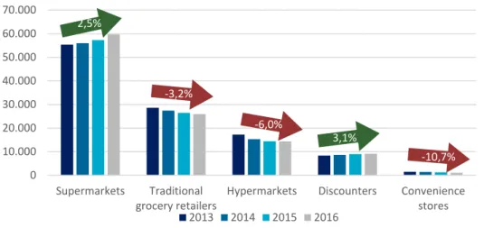
The years of economic recession affected considerably the food retail sector in Spain. With the stagnation of domestic demand, discounters and convenience stores are gaining relevance in the Spanish market with sales growing at a CAGR of 3,1% and 2,5%, respectively, from 2013 to 2016, revealing that consumers are becoming increasingly price-sensitive.

(26)

Figure 3.1 - Sales in Spain grocery retailers by channel, in Million USD (source: Euromonitor)

Spain has a mature and diversified market for food retail, offering a wide range of store formats and channels. The 6 larger groups account for less than 50% of the market share in 2016 and all of them are investing extensively in proximity and convenience formats, as well as in their fresh ranges and “price” image.

Figure 3.2 - Spain grocery retailers market share 2017 (source: Statista)

24,6% 9,1% 8,2% 5,5% 4,3% 3,4% 44,9% Mercadona SA Carrefour SA DIA SA Grupo Eroski Lidl Grupo Auchan Others

According to Euromonitor, private-label (PL) products accounted for 36% of sales in 2014 and their importance is unquestionable. The frequency of store visits and purchases is increasing as consumers prefer to purchase fresh products on a regular basis and seek proximity formats. However, as the Spanish economy recovers branded products are regaining importance. In Portugal, the food retail sector is highly concentrated as the top 5 retail chains have roughly 78% of the market share. The recent economic downturn and the challenges associated with it

0 10.000 20.000 30.000 40.000 50.000 60.000 70.000 Supermarkets Traditional grocery retailers

Hypermarkets Discounters Convenience stores Sales in Spain Grocery Retailers by Channel (in Million USD)

2013 2014 2015 2016 2,5% -3,2% -6,0% 3,1% -10,7%

(27)

have polarized the sector with the two main players (Sonae and Jerónimo Martins) increasing market share.

Figure 3.3 - Portugal grocery retailers market share 2017 (source: BPI Equity Research)

27,0% 26,0% 10,0% 9,0% 6,0% 6,0% 16,0% Sonae Jerónimo Martins Intermaché Lidl DIA Auchan Others

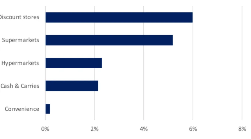
Despite the recent economic recession, food retail sales have proven resilient registering positive growth every year. Discounters and supermarkets have grown at an above 5% CAGR in the past 5 years.

Figure 3.4 - CAGR in grocery retailers in Portugal by channel, 2013-18f (source: Planet Retail)

0% 2% 4% 6% 8%

Convenience Cash & Carries Hypermarkets Supermarkets Discount stores

Portugal: CAGR Growth by Channel, 2013-2018f (%)

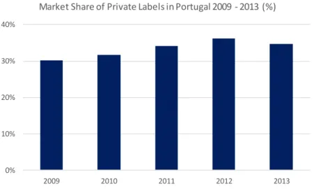
Recent trends include a highly promotion-oriented market and the strategy has revealed effective. National brands have been supporting this promotion intensity and saw their long-term declining trend reverting to private labels. Nonetheless, private labels still represent a significant proportion.

(28)

Figure 3.5 - Market share of private labels in Portugal, 2009-13 (source: Nielsen) 0% 10% 20% 30% 40% 2009 2010 2011 2012 2013

Market Share of Private Labels in Portugal 2009 - 2013 (%)

3.1.2 Emerging Markets

According to McKinsey, Emerging Markets traditional grocery formats have been proven resilient as global grocery giants struggle to find a sustainable strategy to profit from a largely unexplored consumer market. Multinational grocers relied on the modern formats that are working well in the developed world, but the macroeconomic and demographic reality is completely different. Hypermarkets prospered in the developed world thanks to a handful of conditions that emerging markets still do not benefit from in a large scale: affluent consumers, large middle class with decent wages and stable employment, widespread car ownership, among others.

(29)

In Brazil, the grocery retail market is developing and modernizing supported by a young, urban population and a fast-growing middle class. The market is highly fragmented as the largest five players compete with an immeasurable number of small and regional grocery chains. In 2015, according to Planet Retail, the top 10 retailers accounted for less than 40% of the total industry sales, but the market is shifting dynamically.

In 2013, the Brazilian discount sector captured around of 1% of the national grocery spending but it is expanding rapidly with leading discount players like Walmart, DIA and Econ. Private label penetration is low as its sales accounted for just an estimated 5% of consumer spending on food and drink, according to Nielsen research.

Global retailers face the same challenge in Argentina and in Brazil, as traditional formats still dominate the highly fragmented market. However, substantial growth has being seen in the modern grocery retail formats as the economy recovers from recession and deflation. Discounters are growing in popularity with international players rolling out their banners like Carrefour, Casino and DIA.

3.1.3 International trends and the future of grocery retail

Both developed economies and emerging markets face different challenges and opportunities with changing macroeconomic and demographic dynamics. In the Western world, ageing population, low inflation and stagnant growth present the main challenges for food retailers as competition increases. On the other hand, emerging economies present higher growth prospects with the increase of urban population, rise of the middle class and higher disposable income which suggests that modern grocery retailers will have to focus on proximity formats.

Changing consumer habits require constant adaptation from retailers with consumers increasingly more aware of health issues and demanding of fresh products. With this in mind, the market has been increasing its offerings of fresh and perishable products, like meat, fish, vegetables, fruit and bakery, while adapting store concepts to enhance customer experience. The growth of discounters has put pressure on sales due to intense competition, decreased margins which led to cost cutting, ultimately harming innovation. To revert this trend, automation and robotics can substitute labor and increase operating efficiency. Technology can also feed managers with real time date with sensor and predictive analytics

The online grocery retail segment also represents an opportunity for retailers with consumer demand increasing rapidly in recent years. E-commerce improves customer experience by

(30)

finding the optimal balance between the digital platform and the physical infrastructure of bricks and mortar.

3.2 Macroeconomic outlook

3.2.1 Iberia

Spain and Portugal have been considerably affected by the sovereign debt crisis and subsequent recession, which damaged severely the purchasing power of consumers in both countries. In Spain, the burst of the housing market bubble led to a crisis in the banking sector, where the State had to bail out some banks to strengthen their balance sheets. This was followed by a credit crunch that led to unemployment and less disposable income, affecting economic growth.

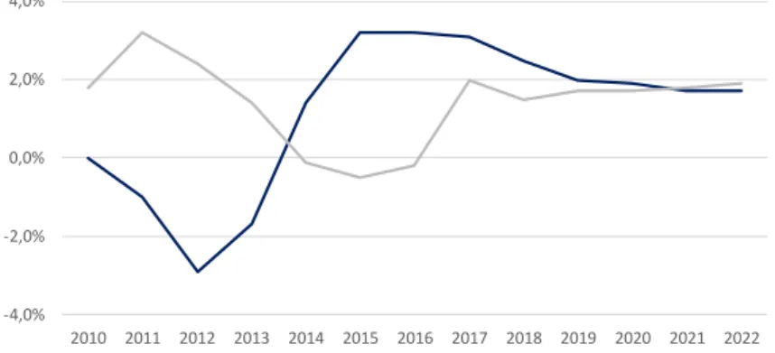
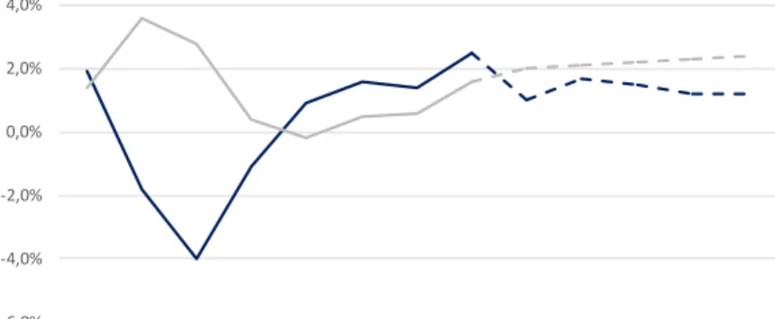
Figure 3.6 - Spain historical and forecasted real GDP growth and inflation (source: IMF)

-4,0% -2,0% 0,0% 2,0% 4,0% 2010 2011 2012 2013 2014 2015 2016 2017 2018 2019 2020 2021 2022 GDP growth, constant price Inflation

From 2009 to 2013, Spanish real GDP growth fell at a 1,4% CAGR. In 2010, the unemployment rate increased to 19,9%, having peaked at 26,1% three years later. Retail food sales decreased at a CAGR of 2,95% between 2008 and 2013, affected by the reduction of purchasing power of the Spanish population.

However, real GDP grew above 3% per annum in the past 3 years and the future seems optimistic with inflation back at normal levels and retail sales growth reflecting consumer confidence. IMF projections until 2022 indicate that real GDP growth and inflation will converge at roughly 2%.

(31)

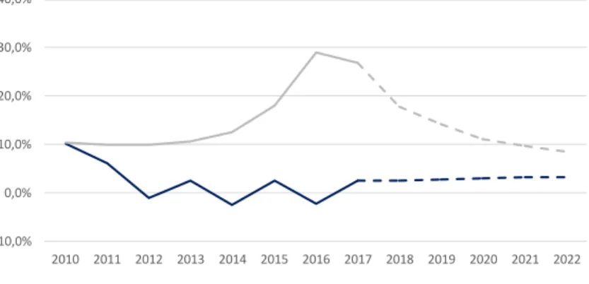
Figure 3.7 - Unemployment rate and retail sales growth in Spain (source: National Statistics Institue of Spain and Bloomberg) -18,0% -12,0% -6,0% 0,0% 6,0% 12,0% 18,0% 24,0% 30,0% 2010 2011 2012 2013 2014 2015 2016 2017

Unemployment rate Retail sales growth

Portugal faced pressure from bonds market, after its credit rating have been downgraded to “junk”, to reduce the budget deficit by raising taxes and reducing public spending. The country was financially rescued and assisted by the IMF and EU in 2011. This inevitably led to a recession, with negative real GDP and retail sales growth, following Spain’s trend, resulting from lower purchasing power.

Figure 3.8 – Portugal historical and forecasted real GDP growth and inflation (source: IMF)

-6,0% -4,0% -2,0% 0,0% 2,0% 4,0% 2010 2011 2012 2013 2014 2015 2016 2017 2018 2019 2020 2021 2022 GDP growth, constant price Inflation

Portugal left the bailout programme in 2014 and regained access to financial markets, and, since then, real GDP growth has been growing at positive numbers and unemployment has been improving. Retail sales grew 3,6% in the past 2 years.

(32)

Figure 3.9 - Unemployment rate and retail sales growth in Spain (source: National Statistics Institute of Portugal and Bloomberg) -12,0% -6,0% 0,0% 6,0% 12,0% 18,0% 24,0% 2010 2011 2012 2013 2014 2015 2016 2017

Unemployment rate Retail sales growth

3.2.2 Emerging Markets

Emerging Markets economies are more volatile with periods of high growth followed by recessions. Argentina is no different to this: real GDP growth in the years between 2013 and 2016 was 2,4%, -2,5%, 2,6% and -2,20%, having increased its GDP in real terms again in 2017 by 2,5%. Since the 2008 financial crisis that growth was essentially propped up by expansionary monetary policies, resulting in double-digit inflation every year since then.

Figure 3.10 - Argentina historical and forecasted real GDP growth and inflation (source: IMF)

-10,0% 0,0% 10,0% 20,0% 30,0% 40,0% 2010 2011 2012 2013 2014 2015 2016 2017 2018 2019 2020 2021 2022 GDP growth, constant price Inflation

IMF projections until 2022 for Argentina are optimistic with real GDP growing around 3% per annum and inflation decreasing to 8,6% in 2022.

Brazil was considered one of the most attractive economies at the beginning of the millennium after the government took steps towards higher market liberalization, increasing business confidence and attracting foreign investment. After the 2008 financial crisis, Brazil recovered from a small recession in the following year with a 7,5% real GDP growth, however rising inflation led the government to ease expansionary policies, throwing the Brazilian economy

(33)

into recession until 2016. Last year, real GDP grew 0,7% and the IMF expects it grew at 2% per annum until 2022.

Figure 3.11 - Brazil historical and forecasted real GDP growth and inflation (source: IMF)

-5,0% 0,0% 5,0% 10,0%

2010 2011 2012 2013 2014 2015 2016 2017 2018 2019 2020 2021 2022 GDP growth, constant price Inflation

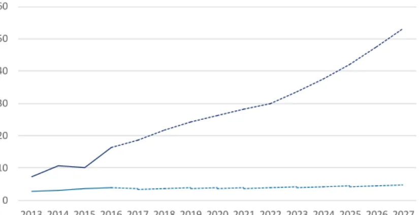
Monetary stimulus in Argentina and Brazil leads to inflation and, thus, devaluation of the currency. From 2012 to 2017, the Argentinean peso and the Brazilian real devalued, on average, 28% and 8% per annum, respectively, against the Euro and this represents the highest risk for foreign investors.

Figure 3.12 - Historical and estimated FX rates for Argentina and Brazil (source: Bloomberg)

0 10 20 30 40 50 60 2013 2014 2015 2016 2017 2018 2019 2020 2021 2022 2023 2024 2025 2026 2027 EUR/ARS EUR/BRL

(34)

4 Company Overview

Distribuidora Internacional de Alimentación, S.A. (DIA) is a Spanish discount supermarket chain founded in 1979. It operates globally and its stores are currently located in Spain, Portugal, Brazil, Argentina and China. It is traded on Spain’s principal stock exchange, Bolsa de Madrid, since July 2011 and it is a member of IBEX-35. In this section, the history of the company, as well as its business strategy, shareholder structure and financial analysis are presented.

4.1 History

In 1979, DIA introduced the first discount store in the Spanish food retail market by opening its first store in Madrid. Five years later, the first DIA-branded product arrived on the shelves, which marked the creation of the company’s corporate image. In 1989, DIA introduced franchise agreements to its business model with the inauguration of the first franchised store. DIA began its expansion in Spanish soil a year later after acquiring Dirsa, followed by the acquisition of Mercadodiario and Ahorro Popular chains in 1991 and 1992, respectively. By that time DIA had already opened more than 1,000 stores throughout Spain. DIA’s internationalization began with the opening of a store in Portugal in 1993. Greece, Argentina and Turkey followed in 1995, 1997 and 1999, respectively, although Argentina remains the only of these countries where DIA operates nowadays. In 2000, DIA merged with the giant multinational retailer Carrefour opening the doors to the French market. DIA continued its expansion strategy with the opening of its first store in China in 2003.

In July 2011 several events marked what was one of the most important years in the Group’s history: the spinoff from Carrefour and the IPO. DIA’s shares were launched in Madrid’s stock exchange for €3,5 apiece implying a market value of equity of €2,378 million. Six months later, DIA debut in IBEX 35 stock market index. The demerger allowed DIA to regain the control of its operations and fully focus on its growth strategy. In 2012 DIA discontinued its operations in Beijing, focusing on Shanghai. A year later, it successfully sold its stake in its Turkish subsidiary and bought Schlecker’s operations in the Iberian market with 1130 stores, improving its proximity home and personal care (HPC) offer, while also diversifying its portfolio. In 2014, DIA sold its French subsidiary for an Enterprise Value of €600 million demonstrating its focus on emerging markets growth and the highly profitable and consolidated Iberian business. In the same year, DIA added more than 600 stores to its portfolio with the acquisition of El Árbol, a

(35)

fresh product specialist, and 160 Eroski stores. In 2017, DIA China operations were discontinued.

By the end of 2017, DIA operated 7.388 stores globally, of which 3.785 are franchised stores and the remaining 3.603 are fully integrated store, 38 warehouses worldwide and employed more than 42 thousand people directly.

4.2 Ownership structure

DIA has 622,456,513 shares outstanding of the ordinary type and same class, entitling their holder to one vote per share. Over 80% of the shares are free-floating and the three major shareholders are: Baillie Gifford & Co. (8,92%), Blackrock Inc. (3,48%) and Black Creek Investment Management Inc. (2,61%), while 1,15% is held as treasury stock and is maintained in the balance sheet in order to cover potential distributions of shares to the Chief Executive Officer and the management team under the Long-Term Incentive Plan for 2016-2018. The Board of Directors is composed by 10 members that in all own 0,256% of the company and the same percentage of the voting rights.

4.3 Business model

DIA is known for being the biggest Spanish discount supermarket chain and it focuses on the retail sale of food, personal care, health and household products, through owned or franchised self-service stores. The company plans to achieve organic growth by consolidating its main market (Iberia) and expanding in the Latin America market. Its strategic advantage is based on a price and proximity (2P) model, with a system of both owned and franchised stores, and strong operational efficiency.

The company benefits from having a very good price image among clients thanks to the minimum cost at which it operates. DIA invests in price to maintain this competitive edge and its private-label brands supports the low-price image among the customers in all geographies. The company currently has almost 8.000 SKUs 1_{in the stores and they represent 46% of the}

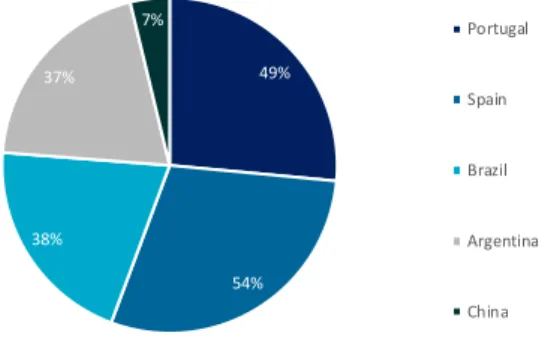
sales, which makes it a core growth driver. The penetration of private-label brands is greater in Iberia than in the Emerging Market, as it is shown in Figure 4.1.

1_{SKUs – Store Keeping Unis}

(36)

Figure 4.1 - DIA private labels by market in 2016 49% 54% 38% 37% 7% _Portugal Spain Brazil Argentina China

DIA also supports the low-price strategy with the loyalty program Club DIA. An initiative created in 1998 that has a reach of more than 37 million customers and gathers their preferences, making it a very useful tool to better manage the supply chain and the commercial offer. 76% of DIA’s total sales were made using the loyalty card in 2016, which indicates the effectiveness of this strategy.

As mentioned earlier, proximity is the second pillar of DIA’s 2P strategy (price and proximity). Approximately 86% of DIA’s network consists of neighborhood stores. Those include:

Figure 4.2 - DIA's neighborhood store network format

Sqm SKU's Main characteristics

DIA Market Minipreço (*)

DIA Fresh Fresh by DIA

Clarel 160 - 260 6000 - Specialized in health, beauty, household and personal care items

Cada Dia Mais Perto

El Árbol La Plaza

(*) Located in rural/urban centres 400 - 700 2800

- Placed in densely neighbourhoods for everyday shopping

- Large range of DIA's products available and perisahbles

150

400 - 1000 2500

- Proximity and closeness to the customer - Specialisation in fresh products and assisted sales in meat and fish in urban areas

n.a.

- Offer essentially based on perishables: fruit, vegetables, meat and fish selections and dairy products

n.a. n.a. - Placed in rural areas, offers the franchisees greater flexibility

DIA diversifies its offer and targets a different type of customer by running larger format stores, which account for the remaining 14% of the store network:

(37)

Figure 4.3 - DIA's larger store network formats

Sqm SKU's Main characteristics

DIA Maxi Minipreço (**)

Max Descuento 1000 n.a. - The cash & carry business line in Spain, specialized in the hotel and restaurant sectors (**) Located in the suburbs of cities

700 - 1000 3500

- Largest store format and includes customer parking

- Adapted to larger and less frequent purchases

Another important differentiating factor of DIA’s business model is its franchise regime that manages 51% of the store network worldwide. DIA cultivates a close relationship with the entrepreneurs from the beginning which is a key to this business model success. DIA’s historical knowledge of the sector combined with its powerful logistics infrastructure as well as the strength of its brand allied with the franchisee local market expertise reflects the success of this business model. DIA currently is the leading franchiser in Iberia, the third in the distribution sector in Europe and the largest franchiser in Argentina, where 70% of the stores are franchises.

DIA combines three categories of stores in its network: COCO (Company Owned, Company Operated), COFO (Company Owned, Franchise Operated) and FOFO (Franchise Owned, Franchise Operated). COCO stores are important to test new concepts before replicating them to franchises and, although they still represent the 49% of the store network, DIA aims to transfer them to the franchised network. COFO stores were introduced in 2006 and DIA assumes the initial investment and then transfers the management of the store to the franchisee, while FOFO was the initial model of franchises of the company.

The process of transferring COCO stores to the franchised models has a positive impact in the financial performance of the company: on the one hand, DIA still acts as the commercial intermediary between suppliers and franchised stores, although “losing” a bit of the gross profit margin to the franchisee; on the other hand, franchisees support operating and personnel expenses (in case of COFO stores, DIA assumes rent expenses) and DIA obtains a higher EBITDA margin with franchised stores compared to COCO ones. This regime may also have some risk and disadvantages attached, because even though franchisees stores are supervised, there is a general loss of control that may result in deviations from the core strategy of the company, resulting in the deterioration of its image amongst clients.

DIA developed an IT system to support its 38 warehouses worldwide. This logistics system is designed to manage the global supply chain, from the supplier to the warehouses and the stores.

(38)

These warehouses, with a total area of almost 770.000 sqm, are placed closed to larger metropolis, resulting in lower fuel expenses.

DIA Group is also undergoing a digital transformation at all levels, whose main goals are approximation to the customer needs and improving efficiency. Optimizing decision-making processes by transforming data in knowledge is at the heart of the improvement of logistics chain processes, efficient store management and better understanding the customer needs. E-commerce projects and commercial digitalization were also central to DIA’s strategy during 2016. DIA online store in currently serves 15 million customers in Spain and its competitive prices and promotional discounts, makes it lowest-priced in the entire company.

4.4 Financial analysis

The financial analysis is based on the data included in the Consolidated Annual Account from the last 5 complete fiscal years, from 2013 to 2017. The analysis is done both by segment and as a group, excluding France since DIA discontinued its operations in the country in 2014.

4.4.1 Operating performance

DIA’s net sales have grown at a CAGR of 2,06% since 2013. Over the same period, total selling area increased from 2,286 million of square meters with 6.463 stores to 2,7681 million square meters with 7.388 stores at a CAGR of 3,4%, implying that net sales per square meter of selling area has decreased.

During the same period, the net profit has decreased from €190,9M to €130,9M which reflects essentially the divestment from France in 2014 and, more recently, the discontinuation of DIA China operations. Following the same trend, operating costs decreased at a CAGR of 3,12% in the last 5 historical years. Operating costs include cost of goods sold, personnel costs and other operating costs. The consolidated income statement is shown in the figure 4.3 and it includes France operations.