Equ
ity
Va
luat
ion
Thes
is
EDP
Renewab
les
D
iogo
Fernandes
D
isser
ta
t
ion
wr
i
t
ten
under
the
superv
is
ion
of
Professor
José
Car
los
Tude
la
Mar
t
ins
Dissertation submittedin partial fulfilment of requirements for the MScin Economics with majorin Finance & banking, at the Universidade Católica
2
Abstract
This dissertation has the intent of valuating EDP Renewables, a subsidiary company from EDP, listed on PSI20, inserted in the Utilities Industry - renewable energy. As a result of the energy sector transformations, fear of fossil fuel shortages and environmental protection, the progressive search for clean sources of power becomes essential to valuate companies that can be game changers.
To estimate the share price the Discounted Cash Flow method was used in both approaches: the Free Cash Flow to the Firm & the Free Cash Flow to Equity, obtaining thus an equity value of €m6.405 and €m6.248 respectively – this converts into a share price of €7.42 and €7.22. Rest on the Dividend Discount Model, the equity value is €m5.428 implying a share price of €6.28. As reported by the Multiples EV/Revenue, EV/EBITDA and Price/CF per share, prices of €8.60, €7.25 and €7.08 were estimated.
Finally a sensitivity analysis was performed due to the uncertainty associated the company’s environment. In conclusion, a final price of 7.11€ per share and a recommend a buy action is in order (actual price: €6.80). As benchmark, valuations from Morgan Stanley (€8.10) and Macquire Research (€6.2) which allowed us to conclude that the value reached in this thesis is in line with the opinion of others financial institutions and provides this dissertation with practical usefulness.
Resumo
Esta dissertação tem o objectivo de avaliar a EDP Renováveis, uma empresa subsidiária da EDP, listada na PSI20. Como resultado das transformações do setor de energia, o medo de escassez de combustíveis fóssil e proteção ambiental, a busca progressiva por fontes limpas de energia torna-se essencial para avaliar as empresas que podem ser crucias no mercado.
Para estimar o preço da ação, o método Discounted Cash Flow foi utilizado nas suas duas abordagens: Free Cash Flow to the Firm & the Free Cash Flow to Equity, obtendo assim um valor de capital próprio de € m6.405 e € m6.248, respectivamente – traduzindo-se num preço de ação de € 7,42 e € 7,22. A partir do modelo de Dividend Discount Model, o valor patrimonial é de €5.428, o que implica um preço de ação de €6.28. Conforme relatado pelos múltiplos EV / Receita, EV / EBITDA e Preço / CF por ação, foram estimados os preços de € 8.60, € 7.25 e € 7.08.
Finalmente, uma análise de sensibilidade foi realizada devido à incerteza associada ao ambiente económico e à Indústria em que empresa se insere.
Em conclusão, um preço final de 7,16 € por ação e uma recomendação para comprar é devida (preço atual: 6,80 €). Como benchmark, as avaliações da Morgan Stanley (€8.10 e da Macquire Research (€6.2) permitiram concluir que o valor alcançado nesta tese está em linha com a opinião de outras instituições financeiras e fornece esta dissertação com utilidade prática.
3
Acknowledgments
The knowledge that I have acquired since the beginning of my bachelor degree until my current work experience compiles the pillars for this dissertation. Although university is much about individual learning and tests, individuality is the last word I would use to describe my path here. Without the help and teamwork of others, this path could never me possible.
This dissertation is dedicated to my parents, for always believing in me and supporting me even if it was hard for them to do so. I wasn’t blessed with a big family, but I was blessed with the best one, for sure. May I ever be as attentive to my children as you were with me.
.
I would also express my gratitude to my supervisor, Professor José Carlos Tudela Martins for his seminars and valuable advices and help during this dissertation; to all the University professors and staff that have taught me so much, both as an academic and as a person. To all of you, my deepest gratitude.
Finally but not the least, I would like to thank Professor António Manuel Simões for teaching me the importance of mathematics in the world and to his incentives and passion for the numbers who were passed to me when I was very young.
5
Contents
1. Literature Review ... 9
1.1. The purpose of Valuation ... 9
1.2. Discounted Cash Flow Methods ... 11
1.2.1. Dividend Discount Model ... 11
1.2.2. Discounted Cash-Flow ... 12
1.2.2.1. Terminal Value ... 14
1.2.3. Adjusted Present Value ... 15
1.3. Profitability Models ... 17
1.3.1. Economic Value Added... 17
1.3.2. Residual Income/Dynamic Return on Equity ... 18
1.4. The Cost of Capital ... 18
1.4.1. The Risk Free Rate ... 18
1.4.2. Capital Asset Pricing Model ... 19
1.4.3. Cost of Equity ... 20
1.4.4. Cost of Debt ... 20
1.4.5. Weighted Average Cost of Capital ... 21
1.5. Relative Valuation ... 21
1.5.1. Multiples Valuation ... 21
1.5.2. Peer Group ... 22
1.6. Option Pricing Theory... 23
2. Macroeconomic Review ... 25
2.1. World Economic Outlook ... 25
3. Industry Overview ... 26
3.1. Industry Leaders ... 26
3.2. Advantages of Renewable Energy ... 27
3.2.1. Green Energy’s Economics of Scale ... 28
4. Company Overview ... 30
4.1. Introduction ... 30
4.2. Stock Performance and Shareholder Structure ... 31
4.3. EDPR Portfolio ... 32
4.4. Operational data and performance ... 32
4.5. Financial data and performance ... 33
4.6. Operational and Financial Data by Region ... 34
6 5.1. Introduction-Models Used ... 36 5.2. Assumptions ... 37 5.2.1. Macro Assumptions ... 37 5.2.1. Industry-specific Assumptions ... 38 5.2.2. Company assumptions ... 38 5.3. Historical Data ... 41 5.4. Forecasts for 2017-2026 ... 44
5.4.1. Main assumptions for 2017 ... 44
5.4.2. Forecasts 2018-2026 ... 45
5.4.3. CAPM Results ... 50
5.4.4. WACC results ... 52
5.4.5. Discounted Cash Flows models – results ... 53
5.4.5.1. Free Cash-Flow to the Firm ... 53
5.4.5.2. Free Cash-Flow to Equity ... 54
5.4.5.3. Dividend-Discount Model ... 55
5.4.6. Multiples results ... 55
5.4.6.1. EV/EBITDA ... 56
5.4.6.2. EV/Revenues ... 57
5.4.6.3. Price/CF per share ... 58
5.5. Different scenarios comparison and resume ... 58
5.6. Sensitivity Analysis ... 60
5.6.1. Single variables ... 60
5.7. Valuation Resume ... 61
5.8. Comparison with other valuations ... 63
6. Conclusion ... 64
7 Table of Figures
Table 1- Share Price Evolution ... 31
Table 2- EDPR stock highlights ... 31
Table 3- EDPR's Portfolio ... 32
Table 4- EDPR Operating data 2014-2016 ... 33
Table 5- EDPR Financial Data 2014-2016... 34
Table 6- Operational and Financial Data for Europe, 2014-2016 ... 35
Table 7- Operating and Financial Data for North America and Brazil, 2014-2016 ... 36
Table 8- GDP growth (% change), 2015-2022 ... 37
Table 9- Inflation (% change), 2015-2022 ... 37
Table 10- Tax Rate (%), 2016-2017 ... 38
Table 11-EDPR's Installed capacity by country, 2008-2016 ... 38
Table 12- Average Load factors (%), 2008-2016... 39
Table 13- Electricity Output, 2008-2016 ... 39
Table 14- Average Selling Price, 2008-2016 ... 39
Table 15- Revenues and EBIT, €m, 2008-2016 ... 40
Table 16- EDPR's Business Strategy 2016-2020 ... 40
Table 17- EDPR's Consolidated Income Statement, 2008-2016 ... 41
Table 18- EDPR's Consolidated Balance Sheet, 2008-2016 ... 42
Table 19- EDPR's Net Financial Expenses, 2008-2016 ... 43
Table 20- EDPR's Capex and Cash-Flow, 2008-2016 ... 43
Table 21- Consolidated Income State and prediction for 2017 ... 44
Table 22 - Consolidated Balance Sheet with forecast for 2017 ... 44
Table 23- Portugal forecasts 2017-2026 ... 45
Table 24- Spain's Forecasts 2017-2026 ... 46
Table 25- Rest of Europe's Forecasts 2017-2026 ... 47
Table 26 - North America's Forecast 2017-2026 ... 48
Table 27- Consolidated Income Statement (m) Forecast 2017-2026 ... 49
Table 28 - Balance Sheet and other Financial Maps 2017-2026 ... 50
Table 29 - CAPM regression statistics ... 51
Table 31 - Equity Beta and WACC calculation steps ... 52
Table 30 - Market risk premium using Fernandez(2017) results ... 52
Table 32 - Free Cash Flow to the Firm (FCFF) and DCF ... 53
Table 34 - Free Cash Flow to Equity, DCF and Equity Value ... 54
Table 33 - Equity Value ... 54
Table 35 - Dividend Discount Model ... 55
Table 36 - EV/EBITDA multiples comparison ... 56
Table 37 - EV/Revenues multiple comparison... 57
Table 38 - Price/CF per share ... 58
Table 39 -EV/EBITDA scenarios ... 59
Table 40 - EV/Revenues scenarios ... 59
Table 41- Price/CF per share scenarios ... 59
Table 42 - Single-variable sensitivity analysis on FInancials ... 60
Table 43 - Share price across models ... 62
8 Table 45 - Valuation Comparison ... 63
9
1. Literature Review
The present and first section of this thesis is a prospectus of the state-of-the-art in equity valuation, gathering and explaining the existing models in order to complete a valuation exercise on EDP Renewables.
That said, all the models here introduced will be thoroughly characterized in concordance with the literature that fundament, exploit and typify their assets and liabilities. It’s essential to mention that, as it will be explained further, some models will be more suitable for the exercise than others, depending on parameters such as capital structure.
Also, some of the methods here explained will have similar objectives, making them almost substitutes. One of the main questions managers struggle to answer is what type of valuation method to use in order to correctly measure their companies value or performance. (Luherman, 1997). For that reason, not every method explained in this part will be used for the actual valuation of this dissertation topic but there will be a selection of the methods which create a more tailor-made path to a correct valuation of this company, taking into account its historical performance, the industry it is inserted and its fundamentals.
1.1. The purpose of Valuation
“There is one principal theme that carries through all of finance. It is value. What exactly is a particular object worth? To make smart decisions, you must be able to assess value—and the better you can assess value, the smarter your decisions will be.”
-Welch (2009) Valuation is not to be regarded as something simple, easy-to-do process. It’s true that most of the work might be somewhat mechanic but the crucial steps, the assumptions one makes and the capacity of the analyst in understanding the company and its positioning in the market is crucial to better valuate the company. Goedhart et. al (2010) insist in having as a ground rule for value creation, a realistic estimation of market opportunities and a keen sense for the industry environment. That said, analysts should first comprehend up to what level external factors may affect the value of the firm so they can, with rigor, specify beneficial investment decisions (Damodaran, 2004). The same author goes further and states that what the
10
understanding of value determinants and the know-how in estimating that value should act almost as a prerequisite for this kind of exercise. (Damodaran, 2006) It’s important to keep in mind that valuation is not timelessly definitive. This implies that, mainly due to shifts in the economic cycle, assumptions made today will not, with high probability, hold in the future (Damodaran, 2002).
“When you do any valuation, there are three possibilities. The first is that you are right and the market is wrong. The second is that the market is right and that you are wrong. The third is that you are both wrong. In an efficient market, which is the most likely scenario?” (Damodaran, The Dividend Discount Model)
Finally it’s imperative to introduce and explain the relevant models for valuation. These are, as said before, different approaches to fulfill the same purpose. In the next few parts of this section, each of these models will be presented and discussed.
Cash Flow
Approaches
Equity Values Dividend Discount Model
Enterprise Values (Equity and debt)
Discounted Cashflow
Returns Based Approaches
Equity Values Dynamic Return on Equity (ROE)
Enterprise Values (Equity and debt)
Economic Value Added Multiples Equity Values Dividend Yield Price to Earnings Ratio Price to Book Value Enterprise Values (Equity and debt)
Free Cash Flow Yield
Enterprise Value to EBIT
Enterprise Value to Capital
Figure 1 - Different types of Valuation Source: Goldman Sachs (adapted)
11
1.2.Discounted Cash Flow Methods 1.2.1. Dividend Discount Model
The Dividend Discount Model is one of the hallmarks in valuation. Dating back to 1938, it was developed by Williams and later revised by Gordon and Shapiro in 1956. This revision caused a mixture in the true creator of this model, since until today, the Dividend Discount Model is commonly known as the Gordon Growth Model.
This model, as its name leads to believe, is based on dividends. It assumes that the only cash flow received from the acquisition of a publicly traded stock is the dividend it provides. This jumps to the underlying conclusion that stock value must reflect the present value of all its expected dividends.
𝑉𝑎𝑙𝑢𝑒 𝑝𝑒𝑟 𝑠ℎ𝑎𝑟𝑒 𝑜𝑓 𝑆𝑡𝑜𝑐𝑘 𝑃0 = ∑ 𝐸(𝐷𝑃𝑆(1+𝑘 𝑡) 𝑒)𝑡 𝑡=∞
𝑡=1
(1)
Where the numerator represent the expected value of dividends per share (DPS) and 𝑘𝑒 the cost of equity.
Gordon and Shapiro revised this model, and assumed that firms would be forever in a steady state, meaning its growth would be constant over time. Damodaran (2005) also presents a two-step model adequate for companies whose growth rate may be somewhat abnormally high for a certain period but will then stabilize forever.
𝑃0 = 𝐸(𝐷𝑃𝑆𝑡) 𝑘𝑒−𝑔 (2) 𝑃0 = ∑ 𝐸(𝐷𝑃𝑆𝑡) (1+ 𝐾𝑒,ℎ𝑔)𝑡 𝑛 𝑡=1 + 𝐸(𝐷𝑃𝑆𝑛+1) 𝐾𝑒,𝑠𝑡−𝑔𝑛 (1+𝐾𝑒,ℎ𝑔)𝑛 (3)
In equation (1), g represents the growth rate of dividends, whereas in equation (2), g is the extraordinary growth in dividends for the first n years, 𝐾𝑒 is the cost of equity (hg is the high growth period and st is the stable growth period), 𝑔 is the extraordinary growth for the first n years and 𝑔𝑛 is the steady state growth for the remaining years.
Alternatively, Molodovsky et al (1965) propose a multistage growth model to correct the assumption of constant growth in the estimation of value. Hence, the
12
methodology follows a three-phase approach with different dividend growth rates. Typically, the growth rate will start as positive but it will linearly decline before reaching a lower constant growth rate that will endure for the rest of the firms live. The classic Gordon Growth Model, although useful and convenient, meets its limitations regarding the assumption of steady state growth. Damodaran (1994) advises that if growth is constant forever, other measures of performance will also be constantly growing, which is not empirically observed for the majority of companies. Also, distributing dividends is a decision that can be based only as to give a signal of strong performance to the market. Furthermore there are companies who opt not to pay dividends at all even if they have a lot of cash surplus. This can be observed in big companies such as Amazon or Google. In these cases it’s impractical and troublesome to compute a reliable valuation using the standard model.
For the two-stage period, some problems may arise. Firstly, it’s hard to find a decision rule for how long the extraordinary period will last. As it is expected a decrease in the growth rate after the first period, a high investment will lead to longer periods. The issue is translating these qualitative assumptions into quantitative realities. Secondly, an abrupt drop in the dividend growth rate from period 1 to period 2 is also somewhat suspicious and inadequate. In reality, the growth rate would decline in a much more steady-paced movement, gradually settling into the period 2 growth rate. Subsequently, there might be skewed results when estimating a firms’ value in a model which dividends are its core foundation and the company does not distribute all the dividends it could, in theory. In such cases, a firm’s value will be undervalued because they decided to accumulate some cash instead of paying it out as dividends.
1.2.2. Discounted Cash-Flow
Havnaer et al (2012) state that this is one of the most widely accepted methods in valuation. In fact, as cash is king (Copeland et al, 2000) and value should be quantified as a function of cash, timing and risk (Luherman, 1997).
To estimate firm value using these methods, a prediction of the present and future cash-flows is needed, along with stable growth risk and an appropriate discount rate
.
13
Within this method, there are two processes by which a firm’s value can be computed: the Free Cash-Flow to the Firm (FCFF) and the Free Cash-Flow to Equity (FCFE).
The FCFF is regarded as the expected value of cash-flows derived from operations, after taxes, before interests being due and including company investments:
𝐹𝐶𝐹𝐹 = 𝑁𝑂𝑃𝐴𝑇 − 𝑇𝑎𝑥𝑒𝑠 + 𝐷𝑒𝑝𝑟𝑒𝑐𝑖𝑎𝑡𝑖𝑜𝑛 𝐸𝑥𝑝𝑒𝑛𝑠𝑒 − 𝐶𝐴𝑃𝐸𝑋 − ∆𝑁𝑊𝐶 (1) The main idea behind this method is that shows the available cash-flow of all participants and as cash is least exposed to tempering (Estridge J. & Lougee B., 2007). So, using the weighted average cost of capital (WACC) as a discount factor, it is possible to compute a valuation of the firm:
𝐹𝑖𝑟𝑚 𝑉𝑎𝑙𝑢𝑒 = ∑ 𝐹𝐶𝐹𝐹𝑡
(1+𝑊𝐴𝐶𝐶)𝑡 𝑁
𝑡=1 (2)
The other perspective of a DCF valuation is somewhat similar to the idea behind the Dividend Discount Model. The available cash to be distributed in dividends should equal the cash-flow of operations net of all payments to debt holders. Hence, using the FCFF as a starting point, it’s possible to compute the FCFE:
𝐹𝐶𝐹𝐸 = 𝐹𝐶𝐹𝐹 − 𝐼𝑛𝑡𝑒𝑟𝑒𝑠𝑡 × (1 − 𝑡) + ∆ 𝑁𝑒𝑡 𝐷𝑒𝑏𝑡 (3)
The objective is now to find the Equity Value. In order to achieve such result, it makes sense to discount all available FCFE to the cost of equity. Hence, Equity Value will be computed in a similar fashion as Firm Value:
𝐸𝑞𝑢𝑖𝑡𝑦 𝑉𝑎𝑙𝑢𝑒 = ∑ 𝐹𝐶𝐹𝐸𝑡 (1+𝑟𝑒)𝑡 𝑁
𝑡=1 (4)
These two approaches should, in theory, output the same results. This seems plausible due to the direct relation between the two paths. Goedhart et al (2005) state the usefulness of these methods, since they can be used to value investments as well as multinational companies.
Nonetheless, these methods also have its downsides. Pinto et al (2010) argued that a company with negative FCFE, is levered or a varying capital structure the FCFF yields a more accurate result since the cost of equity is more sensible to capital structure changes.
14
Also, Luerhman (1997) assert that for complex capital structures, fund raising strategies and tax positions increase the valuation errors. In addition, the author also specifies that the estimation of the weighted average cost of capital is sensible to tax shields, issue costs, debt securities. It’s important to keep in mind that only market values should be used to compute the WACC (Fernández, 2003).
Considering the company chosen for this dissertation, this method will be used, given the usefulness, simplicity and the symbiosis that the method shares with the firm. The disadvantages stated don’t fit with the company’s structure.
One core, transversal question in using this method is to choose a time frame for the projections. Literature typically recommends an explicit period of five to ten years. This period is obviously adaptable, depending on the stableness of the firm. It would be unwise to choose a small window period for a relatively new company which is expanding or a very large period for stable companies.
This method, as of most of valuation, is an art (Titman, 2007). The key to perform a good valuation lies on its assumptions. Damodaran (2002) states that analysts build faulty valuations not due to the calculations, but due to the lack of information, the quality of the assumptions are already faulty. The problems with valuation lie more in the root of the process, not in the more mathematical part of it.
In conclusion, the DCF value will be given by: 𝐷𝐶𝐹 = ∑ 𝐶𝑎𝑠ℎ 𝐹𝑙𝑜𝑤𝑡 (1+𝑟)𝑡 + 𝑇𝑒𝑟𝑚𝑖𝑛𝑎𝑙 𝑉𝑎𝑙𝑢𝑒𝑁 (1+𝑟)𝑁 𝑁 𝑡=1 (5) 1.2.2.1. Terminal Value
Walt Disney once said that “forever is a long time”. Aspects of everyday life are constantly changing and no one can expect that the world will enter in a steady state indefinitely. Intrinsically, the same happens with firms. This section is ought to explain the second part of a DCF valuation, the Terminal Value. Although this method contradicts the premise stated above, it’s impossible to estimate every future cash-flow from today to the end of time, so as a last-resource option, it’s easier and achievable to assume that from some point in the future until infinity, the cash-flow will be stable and growing at a constant rate.
15
There are three approaches to cope with Terminal Value, following Damodaran (2002): the liquidation in the final year of all the firm’s assets and its net worth (after debt payments) in the market; applying market multiples to the company’s earnings or sales revenues from the terminal year, though mixing multiples and DCF approaches may yield biased results; lastly using a stable growth model where there’s a percentage of cash-flow invested every year into new assets – taking the opposite direction of the liquidation model- assuming a steady-state and stable growth for the company.
𝑇𝑒𝑟𝑚𝑖𝑛𝑎𝑙 𝑉𝑎𝑙𝑢𝑒𝑡 =𝐶𝐹𝑡+1
𝑅−𝑔 (6)
The main limitation of this method is the use of a perpetual growth rate. As this rate is fixed and assumed to last forever, it means that the company will always grow more than the world economy (Damodaran, 2005).
“Setting the stable growth rate to be less than or equal to the growth rate of the economy is not only the consistent thing to do but it also ensures that the growth rate will be less than the discount rate. This is because of the relationship between the riskless rate that goes into the discount rate and the growth rate of the economy.” (Damodaran, 2002)
1.2.3. Adjusted Present Value
“APV is value additivity, you can use it to break a problem into pieces that make managerial sense.” (Luehrman, 1997)
The Adjusted Present Value (APV) method appears in the literature as a direct substitute of the Discounted Cash Flow approach. The main idea behind this method is to estimate the value of a firm based only in equity financing and then adding the present value of the expected tax benefits net of bankruptcy costs. This method provides transparency since it’s a two-step separated process which allows for a more clear view of this approach (Luehman, 1997).
𝐴𝑃𝑉 = 𝑃𝑉𝐶𝐹 𝐴𝑠𝑠𝑒𝑡𝑠+ 𝑃𝑉𝐴𝑙𝑙 𝑓𝑖𝑛𝑎𝑛𝑐𝑖𝑛𝑔 𝑠𝑖𝑑𝑒 𝑒𝑓𝑓𝑒𝑐𝑡𝑠 (1) The first step is to perform a valuation exercise as if the company was unlevered (only equity-financed). This is easily estimated by discounting the expected free cash-flow to the firm at the unlevered cost of equity, without forgetting the case where there’s a constant perpetual growth.
16
𝑉𝑎𝑙𝑢𝑒 𝑜𝑓 𝑡ℎ𝑒 𝑢𝑛𝑙𝑒𝑣𝑒𝑟𝑒𝑑 𝑓𝑖𝑟𝑚 =𝐹𝐶𝐹𝐹𝑡(1+𝑔)
𝑟𝑑𝑢−𝑔 (2)
Then, for the second component of the equation above, it’s imperative to compute tax shields, i.e., the expected tax benefits as well as the associated bankruptcy costs. Damodaran (2006) advises choosing the correct tax rate and choosing the right level of debt according to the rate volatility. Plus, if the company has a volatile level of debt, the discount rate is also a factor to be carefully thought of to reach a more accurate present value.
𝑃𝑉𝑡𝑎𝑥 𝑠ℎ𝑖𝑒𝑙𝑑𝑠 =𝐷𝑡∗ 𝑟𝑡∗𝜏𝑡
(1+ 𝑟𝑑)𝑡 (2)
The bankruptcy costs are the negative side of having debt. They can be defined as all the payments that have to be made if the firm is unable to honor their obligations. Regardless of the inexistence of a categorical model to estimate the bankruptcy costs, the part it plays on the estimation of the adjusted present value is still crucial. Using 𝜋a as the probability of default and BC as the present value of the bankruptcy cost, the present value of expected bankruptcy cost can be estimated:
𝐸𝑥𝑝𝑒𝑐𝑡𝑒𝑑 𝐵𝑎𝑛𝑘𝑟𝑢𝑝𝑡𝑐𝑦 𝐶𝑜𝑠𝑡𝑠 (𝐸𝐵𝐶)=𝜋𝑎 ∗BC (3)
The main issue regarding this estimation is that neither the probability of default nor the bankruptcy costs can be calculated directly, meaning the most accurate way of obtaining these parameters is through the use of a proxy.
Altman and Kishore (1998) suggested an estimation of a bond rating for each level of debt and use empirical data of default probabilities for each rating to find the probability of default of the firm. Regarding the bankruptcy costs, literature has focused on the magnitude of different types of costs, concluding that generally the direct costs of bankruptcy are small but the indirect costs, although substantial, vary widely across firms. Shapiro and Titman (1985) speculate that the indirect costs could be as large as 25% to 30% of firm value but provide no direct evidence of the costs. For pre-distressed companies, Branch (2002) estimates this value to be approximately 28%.
17
𝑉𝐿= 𝑉𝑈+ 𝑃𝑉𝑡𝑎𝑥 𝑠ℎ𝑖𝑒𝑙𝑑𝑠+ 𝐸𝐵𝐶 (4)
This method is widely used and is significantly better than the Free Cash-Flow approach when facing a company whose capital structure changes considerably along the investor scope. Regarding the specific case of this dissertation chosen firm, this method doesn’t add accuracy since its historical ratio is essentially stable and its politics also haven’t suffered substantial modifications.
1.3.Profitability Models
1.3.1. Economic Value Added
The Economic Value Added (EVA) is a measure of the excess value that derives from an investment and is obtained through the difference between the company’s cost of capital and return on capital. In a more rigorous definition, it’s estimating a variable that is correlated with the value of the firm, specifically, a risk-adjusted cash-flow variable. This model is considerably simpler than the standard Discount Cash-Flow approach, since it’s a derivation of the model. However, simplicity also punishes results, as this variable is not perfectly correlated with the DCF value. 𝐸𝑉𝐴 = 𝐴𝑓𝑡𝑒𝑟 𝑇𝑎𝑥 𝑂𝑝𝑒𝑟𝑎𝑡𝑖𝑛𝑔 𝐼𝑛𝑐𝑜𝑚𝑒 − 𝐶𝑜𝑠𝑡 𝑜𝑓 𝐶𝑎𝑝𝑖𝑡𝑎𝑙 × 𝐶𝑎𝑝𝑖𝑡𝑎𝑙 𝐼𝑛𝑣𝑒𝑠𝑡𝑒𝑑 (1)
The estimation of the capital invested and the cost of capital are the main variables and should be estimated carefully. The first one depends on the initial capital investment plus the cumulative market value. The latter is the market measure of the cost. One should ignore book values, as they tend to underestimate cost of capital for most firms, especially for highly levered firms. (Damodaran, 2005)
One of the basic principles of finance as a discipline is the concept of net present value rule, which represents the present and future expected cash-flows of an investment, resulting in a measure of value surplus of a given project. Economic Value Added is an extension of this rule (Damodaran, 2005). This enlargement allows for another approach to estimate firm value:
𝐹𝑖𝑟𝑚 𝑉𝑎𝑙𝑢𝑒 = 𝐶𝑎𝑝𝑖𝑡𝑎𝑙 𝐼𝑛𝑣𝑒𝑠𝑡𝑒𝑑𝐴𝑠𝑠𝑒𝑡𝑠 𝑖𝑛 𝑃𝑙𝑎𝑐𝑒+ ∑ 𝐸𝑉𝐴𝑡,𝑎𝑠𝑠𝑒𝑡𝑠 𝑖𝑛 𝑝𝑙𝑎𝑐𝑒 (1+𝑘𝑒)𝑡 𝑡=∞ 𝑡=1 + ∑ 𝐸𝑉𝐴𝑡,𝑓𝑢𝑡𝑢𝑟𝑒 𝑝𝑟𝑜𝑗𝑒𝑐𝑡𝑠 (1+𝑘𝑒)𝑡 𝑡=∞ 𝑡=1 (2)
18
1.3.2. Residual Income/Dynamic Return on Equity
The Dynamic Return on Equity model is a similar approach to the EVA, but it focuses on the equity-side perspective. Firstly, the Return on Equity is a ratio that shows the return of Net Income as a percentage of Shareholder’s equity:
𝑅𝑒𝑡𝑢𝑟𝑛 𝑜𝑛 𝐸𝑞𝑢𝑖𝑡𝑦 =𝑇𝑜𝑡𝑎𝑙 𝐸𝑞𝑢𝑖𝑡𝑦𝑁𝑒𝑡 𝐼𝑛𝑐𝑜𝑚𝑒 (1)
The dynamic ROE compares the return on equity (ROE) with the cost of equity (Ke).
𝑉𝑒𝑞 = 𝐸0 × ∑ 𝐸𝑡−1(1+𝐾×(𝑅𝑂𝐸− 𝐾𝑒) 𝑒)𝑡 𝑛
𝑡=1 (2)
1.4.The Cost of Capital
In every Finance-related course, a key fundamental tool to use is the present value. To calculate it, it’s imperative to use a discount rate, which represents no more than an opportunity cost; to valuate savings, for instance, it’s common to use a bank’s interest rate, since money not spent and stored in a bank will provide interest. On the other hand, for investments and firms, to perform valuation, analysts refer to a discount rate that reflects the opportunity cost of money that could be invested in another project. In a more meticulous way, equity-only financed projects will have a specific cost of equity; if the investment is funded through debt-only, it will yield a so called cost of debt; finally, for projects that use a mixed strategy of funds it’s possible to achieve a weighted average cost of capital. This section goes through all these kinds of cost of capital.
1.4.1. The Risk Free Rate
The risk free rate is perhaps the most common variable to be used in any finance-based analysis, and is a core player in computing the cost of capital.
In principle, this rate cannot have any default or reinvestment risk (Damodaran, 2005). This criterion implies that only government bonds can fulfill these criteria, and not all of them are suitable for it since some governments don’t print their own
19
money. Also, only bonds with the same maturity as the investment horizon should be considered.
Furthermore, according to Koller et al (2005), long-term government bonds in the U.S. and Western Europe show significant (low) covariance with the market. This already provides an estimation error when using those rates since the main assumption for the risk free rate, according to this author, is that the risk free rate should be regarded as the return of a portfolio that has no covariance with the market.
1.4.2. Capital Asset Pricing Model
The Capital Asset Pricing Model (CAPM) is a model developed first by Treynor (1962) as a development of the work of Markowitz (1952) on modern portfolio theory. However, Sharpe (1964) developed the CAPM model as most scholars study today and as it will be presented in this dissertation.
Hence, this model determines the relationship between systematic risk and the expected return of a security:
𝐾𝑒 = 𝑅𝑓+ 𝛽[𝐸(𝑅𝑚− 𝑅𝑓)] (1)
In this manner, 𝛽 is the covariance risk of the security with the market, relatively to market variance, meaning this parameter is the marginal effect each dollar has on the market portfolio.
𝛽𝑠𝑡𝑜𝑐𝑘 = 𝑐𝑜𝑣(𝑅𝑠𝑒𝑐𝑢𝑟𝑖𝑡𝑦;𝑅𝑚𝑎𝑟𝑘𝑒𝑡)
𝑣𝑎𝑟(𝑅𝑚𝑎𝑟𝑘𝑒𝑡) (2)
“The attraction of the CAPM is that it offers powerful and intuitively pleasing
predictions about how to measure risk and the relation between expected return and risk. (…)A risky asset’s return is uncorrelated with the market return—its beta is zero—when the average of the asset’s covariances with the returns on other assets just offsets the variance of the asset’s return. Such a risky asset is riskless in the market portfolio in the sense that it contributes nothing to the variance of the market return. When there is risk-free borrowing and lending, the expected return on assets that are uncorrelated with the market return must equal the risk-free rate.”
20
1.4.3. Cost of Equity
The cost of equity is the minimum rate of return required by investors to enter as part of the equity of the firm. Similarly, it’s an opportunity cost that equals to a return on alternative investment for the same level of risk (Pratt, 2002). Following Brealey and Myers (2000), the expected return on equity can be computed as:
𝑟𝑒 = 𝑟 + 𝜋𝑒 (3)
Where r is the risk-free rate and 𝜋𝑒is the equity risk premium. The most common approach used to estimate cost of equity is the CAPM model, as discussed above and presented in equation (1).
After this parameter is estimated it yields a rate that will be part of the total cost of capital which is the reference and basis to make investment decisions and valuation. It’s fundamental to keep in mind that, in practice, there are some additional
premiums to be added on the cost of capital, either based by historical performance, bias or animal spirits. The models used often miss some important risk factors such as lack of information, survival risk and even illiquidity. These risk should be accessed, measured and added to the estimates of cost of equity.
Damodaran (2001) refers to the common use of the Small Cap Premium, used essentially to value small companies which are prone to be acquired. The author believes that, although most of the companies use this premium today, it doesn’t make it right. In fact, the use of this method started in the 1970s, for academics realized that often the traditional CAPM underestimated expected returns for small market capitalizations.
1.4.4. Cost of Debt
The cost of debt isthe rate a company pays on its current debt. It consolidates the default risk and the market interest rates, reflecting in this manner the cost of borrowing money for a company. This parameter can be estimated similarly to the cost of equity:
𝑟𝑑 = 𝑟 + 𝜋𝑑 (4)
In this estimation process, is worth to remember two rules into how the estimation is done. Firstly, keep it current. The cost of debt should reflect the company’s current default risk, regardless of how different it might have been when the company
21
purchased it debt. This also implies that cost of debt should be updated for today’s risk free rate. Working these two assumptions together the outcome should be to keep away from book interest rate. As it has been stated before, market values provide much accurate results in valuation. Secondly, currency should stay consistent so as not to fall on differences in expected inflation. (Damodaran, 2016).
1.4.5. Weighted Average Cost of Capital
Combining the cost of equity and cost of debt, it’s possible to compute, for any given firm, the Weighted Average Cost of Capital (WACC). Following Fernández (2011), “The WACC is just the rate at which Free Cash Flows must be discounted to
obtain the same result as in the valuation using Equity Cash Flows discounted at the required return to equity.”
𝑊𝐴𝐶𝐶 = 𝐸
𝐸+𝐷× 𝐾𝑒+ 𝐷
𝐸+𝐷× 𝐾𝑑× (1 − 𝑇) (5)
Although useful and widely used, this models has its drawbacks. Luerhman (1997) argues that for companies with complex tax structure, the WACC performs poorly. Also, literature strongly punishes this model as one of its main assumptions is that the company has a stable capital structure, otherwise the rate it provides doesn’t properly reflect the cost of capital.
1.5. Relative Valuation
The methods for valuation described until now have as a common basis finding value through their given cash-flows, growth or risk characteristics. Relative Valuation takes a different approach to estimate the value of assets, based on the similarities of assets that are currently priced in the market (Larsen, 2012). Its main assumption is that it relies on the market being right on average but wrong on the pricing of individual stocks. In a first approach, multiples valuation as described below will be helpful so as to correct these errors (Damodaran, 2012).
1.5.1. Multiples Valuation
This type of valuation is one of the most used methods in valuation by analysts and academics. Goedhart et al. (2003) alerts for the often misuse of multiples in valuation as it’s difficult in a comparative analysis to find the “fair” firm to compare. Also, using the industry is often a mistake, as the average doesn’t mean much if the variance of performance is too high. The author then advises four basic principles to correctly use multiples valuation: peers with similar prospects for
22
ROIC and growth, forward-looking multiples, use of enterprise-value multiples and adjustment of the latter for non-operative items.
Although there is some debate about which multiples to use, Lie (2002) infers that it’s always better to consider several multiples – the more the merrier.
𝑃𝑟𝑖𝑐𝑒/𝐸𝑎𝑟𝑛𝑖𝑛𝑔𝑠 =𝐶𝑢𝑟𝑟𝑒𝑛𝑡 𝑀𝑎𝑟𝑘𝑒𝑡 𝑃𝑟𝑖𝑐𝑒𝐸𝑎𝑟𝑛𝑖𝑛𝑔𝑠 𝑝𝑒𝑟 𝑆ℎ𝑎𝑟𝑒 (1) 𝐸𝑛𝑡𝑒𝑟𝑝𝑟𝑖𝑠𝑒 𝑉𝑎𝑙𝑢𝑒 𝑀𝑢𝑙𝑡𝑖𝑝𝑙𝑒𝑠 =𝐸𝐵𝐼𝑇𝐷𝐴 𝑜𝑟 𝑆𝑎𝑙𝑒𝑠 𝑜𝑟 𝐸𝐵𝐼𝑇 𝑜𝑟 𝐶𝑎𝑝𝑖𝑡𝑎𝑙𝐸𝑉 (2) 𝑃𝑟𝑖𝑐𝑒 𝑡𝑜 𝐶𝑎𝑠ℎ 𝐹𝑙𝑜𝑤 =𝐶𝑎𝑠ℎ 𝐹𝑙𝑜𝑤 𝑝𝑒𝑟 𝑆ℎ𝑎𝑟𝑒𝑆ℎ𝑎𝑟𝑒 𝑃𝑟𝑖𝑐𝑒 (3) The price-to-earnings ratio is a broadly known multiple. Fernández (2001) cites this and the Enterprise Value multiples as the most important ones to use in a valuation. Literature advises that different industries will have more suitable multiples than others; a great critique to the P/E ratio, for instance, is that it is distorted by different capital structures of firms and the embodiment of non-operating gains and losses in final result.
1.5.2. Peer Group
Finding a peer group to value a target firm it’s a very demanding task, especially because it’s not easy, even in the same industry, finding similar companies in all relevant characteristics (Henschke and Homburg, 2009). First things first, how can an analyst define industry? Some companies that are within the same industry according to the Standard Industrial Classification (SIC) codes are not comparable because their business is very different or have disparate business models (Koller et al, 2005). However, to define a set of comparable firms it’s desirable to use a statistical tool, like the cluster analysis, or simply the disclosed information that companies make available in their annual reports regarding their peers.
No matter what tool the analyst chooses to use, it’s necessary to have a carefully thought peer group. Literature varies a lot in the definition of what is a “good” peer group. Damodaran (2006) argues that comparable firms should have similar cash flows and level of risk while maintaining the same growth pattern. Koller et al (2005) on the other hand, states that return on invested capital and growth in the long run are more decisive factors. Simply enough, it seems somewhat logic that
23
companies that face the same industry and are involved in the same macro-economic environment are more prone to output a fairly more accurate valuation, qualifying them as excellent peers (Lieu et al, 2002 and Foushe et al, 2012).
1.6.Option Pricing Theory
The basic principle of most of the valuation techniques present until now are based on the fact that the value of any asset is the present value of all future cash flows. Option pricing theory is an exception in the way it approaches assets in two different points of view: assets derive their value from other assets’ values and on the occurrence of specific events cash flows are unforeseen.
Options are derivative contracts which give their owner the right (but not the obligation) to buy (in case of call options) or sell (put options) assets at a predetermined price for a prearranged period of time. They provide flexibility and create value when the cost of the option is lower than the benefits it brings.
According to Copeland et al (1990) options are one of the methods to better manage risk and uncertainty. If an asset is constantly exposed to risk and henceforth is volatile, a manager can protect some of that risk using options. A good example is airline companies. There is a great dependence between oil prices and jet fuel which in turn has a big influence on airlines operations. Options on oil are a common way which big airline companies use to protect themselves against the increase of oil prices.
It’s important to keep in mind that although this method brings a lot of benefits it should not be used as single valuation method; its main use is to complement other types of valuation, acting as a “check point” (Lueherman, 1997).
Option pricing theory dates back to 1972, following the works of Fisher Black and Myron Scholes who first created the now famous Black-Scholes model, using a “replicating portfolio” – a portfolio that is only composed by the asset in study another risk-free asset. Their work also made a breakthrough on the notion of arbitrage, i.e. no-risk investments. A simpler model was then developed, based on the formulation that an asset price will either move up or down in the future; this model, named the Binomial model assumes that the stock price follow a binomial process. Damodaran (2006) suggests that the present value of an option should reflect expectations about its future price, which is a direct aftermath of arbitrage.
24
Binomial Model
Black Scholes Model
S - current value of the underlying asset K - strike price of the option
t - option expiration life r - risk free interest rate
- variance of the underlying asset 𝑆𝑢 𝑆 𝑆𝑑 𝑆 𝑆𝑢 𝑆
S is the current stock price and moves up to Su with probability p and moves down to Sd with probability 1- p.
In limit, the Binomial model, which suffers from discrete changes in prices, will converge to the Black-Scholes Model, a non-discrete approach to price option. Luherman (1997) advises the use of the latter since it shares more inputs with the classical DCF valuation, permitting a fairer, homogeneous comparison.
25
2. Macroeconomic Review
This chapter has the solely objective of providing illustrative data about the general state of the macroeconomic and financial environment with particular emphasis on the utilities sector, acting as a background agent for the valuation assumptions that are going to be used for the specific case of EDP Renewables.
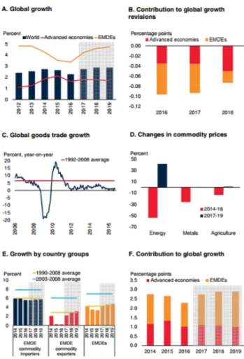
2.1. World Economic Outlook
The past year was marked as the worst since the global financial crisis by the World Bank. 2016 was notable for stalling global trade, poor investment and a fierce policy uncertainty. Results presented by this institute state that global growth has fallen to 2.6 percent in 2016 which represents a 0.1 percentage point below June 2016 forecasts. Although facing such deficient results, 2017 aims for some room improvement, counting on a rise to 2.7 percent, due mostly to emerging markets and developing economies (EMDEs). However developed economies will continue to struggle against growth and low inflation as a direct result of increased risk in policy, unfertile investment and dull productivity growth. As a result, the World Banks points to a 1.6 percent growth in these economies in 2016 and an average of 2.2 percent in 2017.
26
3. Industry Overview
Awareness for the world’s future energy is rising since the beginning of the century and concerns almost every big player in the market: governments, private industrial companies from several industries, financial sector and others. Furthermore, the need for energy is also increasing, with an estimating growth of over 40% between 2012 and 2040.1
Graph 1-Evolution of the world's energy consumption2
Taking into account not only the fact that fossil fuels such as coal or oil are somewhat finite but also the severe climatic changes registered in the past decade, renewable energies can be seen as a strong bet to solve these two problems. In fact, there has already been a clear positive trend in the use of renewable energy.
3.1. Industry Leaders
The reference index for renewable energy is the RENIXX 30, containing, by market capitalization, the top thirty major companies operating in the business. Both the U.S. and China dominate this index
The top thirty major players are ranked by market capitalization in the Renewable Energy Industrial Index (RENIXX 30).
1 Intergovernmental Panel on Climate Change 2016 2 U.S. Energy Information Administration 2016
27
Figure 3- Renewable Energy Industrial Index by market capitalization, April 2017
Source :Renewable-Energy-Industry.com and Thomson Reuters 3.2. Advantages of Renewable Energy
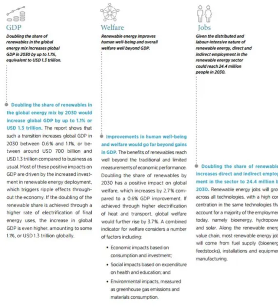
The accelerating change to an energy system based on renewable energy is regarded as a one-of-a-kind chance to satisfy not only the growing energy demand and climate goals but also enhancing human welfare. According to the International Renewable Energy Agency, investing in renewable energy is part of the plan of 164 countries that will contribute to achieve the Paris agreement on climate in 2030. The Agency’s updated report “Renewable Energy Benefits: Measuring the Economics” predicts a 100% increase on renewable energy share on global energy production in the next 13 years, resulting in a global GDP increase up to 1.1 percent, an enhanced 3.7 percent in welfare (measured through 3 sub-indicators: economical, social and environmental, using variables such as consumption, total employment
Company Name Country of Origin Sales (€m)
Albioma SA FR 367.8
Bourbon SA FR 1,020.6
Brookfield Renewable LP BM 2,452.0
Canadian Solar Inc CA 2,853.1
CGG SA FR 1,20
China High Speed Group Co. CH 8,966.0
China Longyuan Power CH 17,87
Dong Energy A/S DN 57,39
EDP Renovaveis SA PT 1,453.2
First Solar Inc USA 2,951.3
Gamesa Corporation Tech SP 4,61
Innergex Renewable Energy CA 292.8
JA Solar Holdings Co Ltd CH 15,74
JinkoSolar Holding Co Ltd CH 21,40
Meyer Burger Technology SW 453.1
Nordex SE DE 3,40
Ormat Technologies Inc USA 662.6
Plug Power Inc USA 85.9
REC Silicon ASA NO 271.2
SMA Solar Technology AG DE 946.7
SolarCity Corp USA 399.6
Solaredge Technologies Inc IL 240.0
SunPower Corp USA 2,559.6
Sunrun Inc USA 453.9
Tesla Motors Inc USA 7,000.1
Trina Solar Ltd CH 3,035.5
Verbund AG AT 2,61
Vestas Wind Systems A/S DN 10,24
Xinjiang Goldwind Science & Tech Co. Ltd CH 26,40
28
and greenhouse gas emissions), and more than 24 million new jobs created on this sector. These are the main three elements that will change with the global attention that’s being put on renewable energy, as the previously mentioned report states:
Figure 4- Three key changing elements with the investment in Energy
Source - Renewable Energy Benefits: Measuring the Economics (IREA; 2016)
3.2.1. Green Energy’s Economics of Scale
The evolution of technology as an economic term has always helped decreasing costs and the energy sector feels no different. In fact, for the past 6 years, the world has seen the cost of implementing green energy decrease further and further, resulting in an increase of investments in the sector.
29
Source - Bloomberg
30
4. Company Overview 4.1. Introduction
EDP Renewables is a Portuguese company that focuses on value creation within the renewable energy sector. It builds and explores wind farms and solar power plants since 1996 and is already expanded to eleven other countries (Spain, France, Italy, Poland, Belgium, Romania, UK, Canada, USA, Mexico and Brazil). Its European headquarter is based in Madrid and its American counterpart is located in Houston. In 2016, the company produced 24,5TWh of electricity, avoiding 20,1mt of Co2 emissions and managing 10,4GW of installed capacity, while employing over than 1000 collaborators.
31
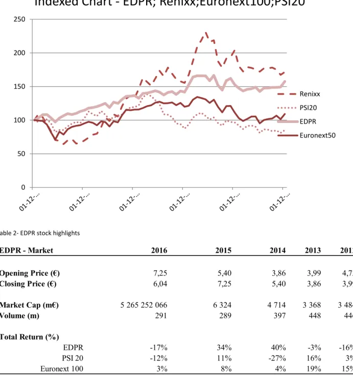
4.2. Stock Performance and Shareholder Structure
EDPR launched its IPO in 2008 and it’s now listed in the Euronext Lisbon. There are 872.380.160 shares outstanding, of which 77.5% belong to EDP S.A., followed by MSF Investment Management with 3,1%. The remaining shares are branched throughout 23 countries
Table 1- Share Price Evolution
Table 2- EDPR stock highlights 0 50 100 150 200 250
Indexed Chart - EDPR; Renixx;Euronext100;PSI20
Renixx PSI20 EDPR Euronext50 EDPR - Market 2016 2015 2014 2013 2012 Opening Price (€) 7,25 5,40 3,86 3,99 4,73 Closing Price (€) 6,04 7,25 5,40 3,86 3,99 Market Cap (m€) 5 265 252 066 6 324 4 714 3 368 3 484 Volume (m) 291 289 397 448 446 Total Return (%) EDPR -17% 34% 40% -3% -16% PSI 20 -12% 11% -27% 16% 3% Euronext 100 3% 8% 4% 19% 15%
32
4.3. EDPR Portfolio
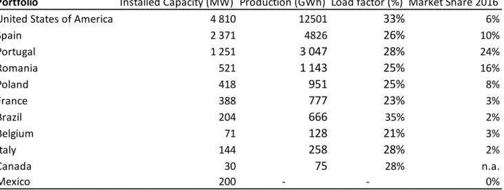
This company’s portfolio is well expanded, operating in 13 countries, with the U.S., Spain and Portugal being its largest business areas in terms of installed capacity and production.
Table 3- EDPR's Portfolio
Portfolio Installed Capacity (MW) Production (GWh) Load factor (%) Market Share 2016
United States of America 4 810 12501 33% 6%
Spain 2 371 4826 26% 10% Portugal 1 251 3 047 28% 24% Romania 521 1 143 25% 16% Poland 418 951 25% 8% France 388 777 23% 3% Brazil 204 666 35% 2% Belgium 71 128 21% 3% Italy 144 258 28% 2% Canada 30 75 28% n.a. Mexico 200 - - 0%
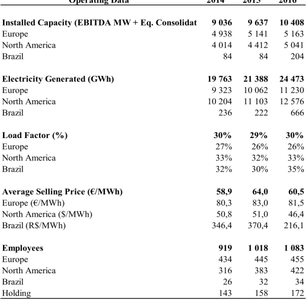
4.4.Operational data and performance
EDPR has a well diversified portfolio across Europe and the American Continent. Its employees are increasing every year, though in very small changes, mainly due to the North America branch. Regarding the Installed Capacity, Europe has been leading with an advantage of 24% over North America in 2016. Also, within Europe, Spain has the biggest installed capacity at 44% of all the European business, followed by Portugal.
On the other hand, North America has been generating more electricity in the past 3 years, holding an average of 51% per year of all electricity generated by the firm. The load factor has been somewhat stable, with small changes across the different business areas, with highlights to Brazil which had a 5% load factor increase from 2015 to 2016.
The average selling price for the different areas of business have also not varied significantly. On average, the price per MWh has been around €61, with small fluctuations on all areas of activity.
33 Table 4- EDPR Operating data 2014-2016
Operating Data 2014 2015 2016
Installed Capacity (EBITDA MW + Eq. Consolidated) 9 036 9 637 10 408
Europe 4 938 5 141 5 163 North America 4 014 4 412 5 041 Brazil 84 84 204 Electricity Generated (GWh) 19 763 21 388 24 473 Europe 9 323 10 062 11 230 North America 10 204 11 103 12 576 Brazil 236 222 666 Load Factor (%) 30% 29% 30% Europe 27% 26% 26% North America 33% 32% 33% Brazil 32% 30% 35%
Average Selling Price (€/MWh) 58,9 64,0 60,5
Europe (€/MWh) 80,3 83,0 81,5 North America ($/MWh) 50,8 51,0 46,4 Brazil (R$/MWh) 346,4 370,4 216,1 Employees 919 1 018 1 083 Europe 434 445 455 North America 316 383 422 Brazil 26 32 34 Holding 143 158 172
4.5.Financial data and performance
In 2016, Revenues increased by almost 7% against the observed value for the previous year. EBITDA has also been successively increasing over the last 3 years. The EBITDA margin decreased 3% in 2016, but it is value is still considerably high: for every euro generated in revenues, around 71 cents are profits before all taxes and paid interests.
On another measure, net profits heavily diminished in 2016 due to the increase in net financial expensive (18%) and the decrease in the EBIT of about 3%. The Operating Cash Flow has been consistently increasing, standing at €564m in 2016.
34
These changes are mainly due to EDPR’s asset rotation strategy3. Capital Expenditures have also been increasing up to €1029m, which are a direct result of the investments made mostly in the North American markets (81%). Net debt decreased 25% due to tax equity deals4 a lower cost of debt which resulted from a renegotiation with EDP and forex differences.
Table 5- EDPR Financial Data 2014-2016
Financial Data (€m) 2014 2015 2016
Revenues 1 276,7 1 547,1 1 650,8
Operating Costs & Other Operating Income (373,5) (404,8) (479,8)
EBITDA 903,2 1 142,3 1 171,0
EBITDA / Revenues 71% 74% 71%
EBIT 422,4 577,8 564,0
Net Financial Expenses (249,9) (285,5) (350,1)
Net Profit (Equity holders of EDPR) 126,0 166,6 56,3
Operating Cash-Flow 707 701 869
Capex 732 903 1 029
PP&E (net) 11 013 12 612 13 437
Equity 6 331 6 834 7 573
Net Debt 3 283 3 707 2 755
Institutional Partnership Liability 1 067 1 165 1 520
4.6. Operational and Financial Data by Region
Taking a closer look by region, the most evident result is that Spain is the main market in Europe in both the operating and financial parts of the business. However this lead is softened in the financial part, since, although Spain has the highest revenue in the Europe side of EDPR’s portfolio, its EBITDA stays somewhat in par with the rest of the continent. It’s important to mention that from 2016 forward, EDPR expects to invest more in the rest of Europe, since Spain and Portugal have already met the market’s need.
3 Selling small assets which are foreseen to become in distress and re-investing its value into more
favorable projects.
35 Table 6- Operational and Financial Data for Europe, 2014-2016
Portugal 2014 2015 2016
Installed Capacity (MW) 624 1 247 1 251
Load Factor (%) 30% 27% 28%
Electricity Output (GWh) 1 652 1 991 3 047
Revenues(m€) 165,7 190,2 267,7
Operating costs and Other operating income (m€) (31,4) 87,6 (44,5)
EBITDA (m€) 134,4 277,8 223,2 EBITDA / Revenues (%) 81% 146% 83% Spain 2014 2015 2016 Installed Capacity (MW) 2 194 2 194 2 194 Load Factor (%) 28% 26% 26% Electricity Output (GWh) 5 176 4 847 4 926 Revenues(m€) 344,8 375,4 348,6
Operating costs and Other operating income (m€) (118,1) (126,0) (122,6)
EBITDA (m€) 226,7 249,4 226,0 EBITDA / Revenues (%) 66% 66% 65% Rest of Europe 2014 2015 2016 Installed Capacity (MW) 1 413 1 523 1 541 Load Factor (%) 24% 27% 25% Electricity Output (GWh) 2 495 3 225 3 257 Revenues(m€) 233,8 272,0 268,1
Operating costs and Other operating income (m€) (65,0) (93,0) (73,7)
EBITDA (m€) 168,8 179,0 194,4
EBITDA / Revenues (%) 72% 66% 73%
Moving to the American continent, Brazil is showing some results, with its EBITDA margin increasing substantially every year. On the Operating side, the country has also increased its installed capacity to 204MW in 2016 from a shallow 84MW in 2015. According to the 2016 report, EDPR is now heavily focusing investments in Brazil, has it has revealed to be investment-worthy and it will continue to be one of the main investment areas in the foreseeable future.
On North America, the installed capacity doesn’t grow at the same pace as Brazil, but it has seen a 14% increase in 2016. The investments in this region will also continue to grow since there is an estimated increased demand for renewable power plants.
36 Table 7- Operating and Financial Data for North America and Brazil, 2014-2016
North America 2014 2015 2016
Installed Capacity (MW) 3 835 4 233 4 861
Load Factor (%) 33% 32% 33%
Electricity Output (GWh) 10 204 11 103 12 576
Revenues(m€) 671,8 772,1 780,5
Operating costs and Other operating income (m€) (217,1) (281,2) (251,1)
EBITDA (m€) 477,4 512,7 555,1 EBITDA / Revenues (%) 71% 66% 71% Brazil 2014 2015 2016 Installed Capacity (MW) 84 84 204 Load Factor (%) 32% 30% 35% Electricity Output (GWh) 236 222 666 Revenues(m€) 78,5 79,1 132,6
Operating costs and Other operating income (m€) (30,8) (35,9) (41,8)
EBITDA (m€) 47,7 45,5 96,7
EBITDA / Revenues (%) 61,0% 58,0% 73,0%
5. EDPR Valuation
5.1. Introduction-Models Used
After reviewing the most used models among the literature, it’s crucial to choose which are the more appropriate. Not all models will be applied for the purpose of this valuation because some of them are somewhat substitutes and others for one reason or another will not be a good fit for the type of company this dissertation is exploring. The DCF method seems a good starting point: it’s widely accepted within the literature and although in some cases, due to the structure of the company, it may not be the most suitable one, EDPR does not pose a threat for the accuracy of this method and henceforth it shall be used. By principle, the WACC shall also be estimated.
The DDM is the second obvious choice: the company pays regular dividends and their value is kept consistently so there aren’t any precautions in poor estimations using this method.
A Relative valuation using multiples is also going to be used. In the sector of Utilities, in which this company is inserted, it has already been covered that some multiples perform better than others. Nonetheless, the method has a large support in the literature and will be considered.
37
Using all these methods, it’s also important to conciliate them with the macro and micro economic environment currently felt by the firm. In the next parts of this chapter assumptions will also be discussed so that they can be properly introduced in a technical financial model.
One final note is to never forget the true purpose of this dissertation: to estimate a price per share for EDPR and recommend an investment on it.
5.2. Assumptions
5.2.1. Macro Assumptions
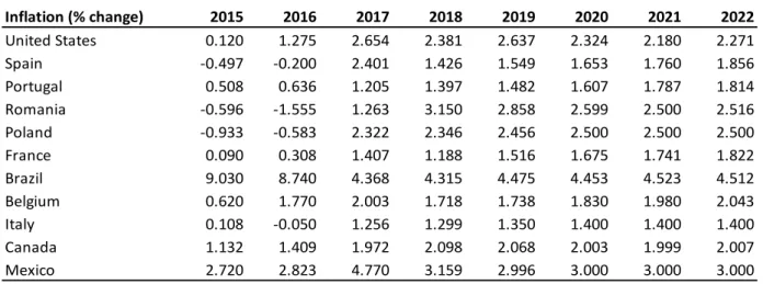
Although there is a chapter about the world’s economic performance, one should specify and adjust this analysis for the specific case of EDPR. In the tables below, one can observed the estimated GDP growth5 and inflation for the countries were EDPR has business activities.
Table 8- GDP growth (% change), 2015-2022
GDP growth (% change) 2015 2016 2017 2018 2019 2020 2021 2022 United States 2,596 1,616 2,307 2,519 2,121 1,825 1,672 1,703 Spain 3,203 3,203 3,203 3,203 3,203 3,203 3,203 3,203 Portugal 1,596 1,432 1,741 1,454 1,16 1,06 0,96 0,99 Romania 3,938 4,785 4,2 3,4 3,3 3,3 3,3 3,3 Poland 3,941 2,83 3,405 3,232 2,992 2,924 2,766 2,71 France 1,274 1,213 1,396 1,65 1,749 1,796 1,83 1,858 Brazil -3,769 -3,595 0,165 1,748 1,954 2 1,998 1,993 Belgium 1,5 1,239 1,633 1,505 1,477 1,544 1,502 1,524 Italy 0,783 0,88 0,843 0,815 0,8 0,8 0,85 0,85 Canada 0,942 1,433 1,941 1,956 1,843 1,8 1,8 1,8 Mexico 2,629 2,302 1,664 1,957 2,71 2,682 2,743 2,708
Table 9- Inflation (% change), 2015-2022
Inflation (% change) 2015 2016 2017 2018 2019 2020 2021 2022 United States 0.120 1.275 2.654 2.381 2.637 2.324 2.180 2.271 Spain -0.497 -0.200 2.401 1.426 1.549 1.653 1.760 1.856 Portugal 0.508 0.636 1.205 1.397 1.482 1.607 1.787 1.814 Romania -0.596 -1.555 1.263 3.150 2.858 2.599 2.500 2.516 Poland -0.933 -0.583 2.322 2.346 2.456 2.500 2.500 2.500 France 0.090 0.308 1.407 1.188 1.516 1.675 1.741 1.822 Brazil 9.030 8.740 4.368 4.315 4.475 4.453 4.523 4.512 Belgium 0.620 1.770 2.003 1.718 1.738 1.830 1.980 2.043 Italy 0.108 -0.050 1.256 1.299 1.350 1.400 1.400 1.400 Canada 1.132 1.409 1.972 2.098 2.068 2.003 1.999 2.007 Mexico 2.720 2.823 4.770 3.159 2.996 3.000 3.000 3.000
5 For the purpose of valuation, a single GDP growth rate will be considered. It will be the weighted
average of all growth rates, weighted by the Installed Capacity for each country.
Source: WEO April 2017
Source: WEO April 2017 Weighted average : 2,03
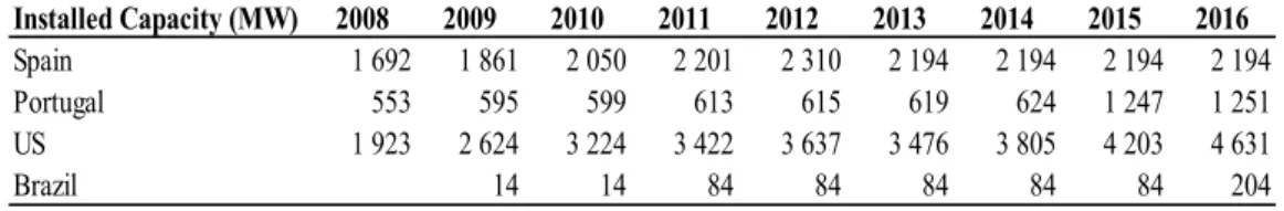
38 Installed Capacity (MW) 2008 2009 2010 2011 2012 2013 2014 2015 2016 Spain 1 692 1 861 2 050 2 201 2 310 2 194 2 194 2 194 2 194 Portugal 553 595 599 613 615 619 624 1 247 1 251 US 1 923 2 624 3 224 3 422 3 637 3 476 3 805 4 203 4 631 Brazil 14 14 84 84 84 84 84 204
Focusing on Table 10, one can observe the current and expected values for tax rates across countries in which EDPR is operating. Although most values are stable, some remarks have to be made, as the CIT laws have been changed:
1. In Italy, starting from 2017, the applicable tax will be 24% instead of 27,5% 2. In France, a reduction of tax has also been approved, starting from April 2017. 3. In the U.K., starting also in 2017 the tax will be 18% which will be further reduced
to 17% in 2021 onwards.
Table 10- Tax Rate (%), 2016-2017
Tax Rate (%) 2016 2017 2018 2019 2020 2021 2022 Belgium 33,99 33,99 33,99 33,99 33,99 33,99 33,99 France 33,33 28 28 28 28 28 28 Italy 27,5 24 24 24 24 24 24 Poland 19 19 19 19 19 19 19 Portugal 21 21 21 21 21 21 21 Romania 16 16 16 16 16 16 16 Spain 25 25 25 25 25 25 25 United Kingdom 20 18 18 18 18 17 17 Brazil 34 34 34 34 34 34 34 Canada 26,5 26,5 26,5 26,5 26,5 26,5 26,5 Mexico 30 30 30 30 30 30 30 United States 38,2 38,2 38,2 38,2 38,2 38,2 38,2 5.2.1. Industry-specific Assumptions
Although having an understanding about the state of the global economy is important for valuation, one also has to follow a top-down approach, i.e., analyzing industry-specific data to better understand what the company faces6. In case of EDPR, Utilities and Renewables seem to be the best fit.
5.2.2. Company assumptions
Moving into a more in depth analysis, the next tables are concerned with EDPR’s historical performance.
Table 11-EDPR's Installed capacity by country, 2008-2016
6 Please refer to annexes for a more detailed information
39 Load Factors (%) 2008 2009 2010 2011 2012 2013 2014 2015 2016 Spain 26% 26% 27% 25% 27% 29% 28% 26% 26% Portugal 27% 28% 29% 27% 27% 29% 30% 27% 28% RoE 23% 23% 24% 23% 24% 25% 24% 27% 25% US 34% 32% 32% 33% 33% 32% 33% 32% 33% Brazil - 22% 26% 35% 31% 31% 32% 30% 35% Electricity Output (GWh) 2008 2009 2010 2011 2012 2013 2014 2015 2016 Spain 2 634 3 275 4 355 4 584 5 106 5 463 5 176 4 847 4 926 Portugal 1 028 1 275 1 472 1 391 1 444 1 593 1 652 1 991 3 047 RoE 238 426 804 1 326 1 727 2 132 2 495 3 225 3 257 US 3 907 5 905 7 689 9 330 9 937 9 769 10 145 11 030 12 501 Brazil - 26 31 170 231 230 236 222 666
Table 12- Average Load factors (%), 2008-2016
Table 13- Electricity Output, 2008-2016
These three tables are operational indicators. Regarding installed capacity and electricity output there is a clear positive trend for all countries. The load factor7 is highly dependent of technology and it indicates the volatility of consumption, i.e., the lowest the factor, the more volatile it is. For the general case, all countries have an average load factor between 20% and 30% meaning they have good potential of investment.
Table 14- Average Selling Price, 2008-2016
7 Average load divided by the peak load in a specified period of time.
Average Selling Price 2008 2009 2010 2011 2012 2013 2014 2015 2016
Spain 100,72 84,04 79,13 82,53 87,71 80,28 50,33 48,73 60,18
Portugal 93,8 94,5 93,8 98,7 101,8 99,3 98,3 95,0 88,0
RoE 70,7 89,7 93,8 95,7 107,2 104,8 95,8 86,0 83,3
US 108,9 82,2 84,9 80,9 82,8 84,5 93,6 95,7 83,0
40 Revenues (€m) 2008 2009 2010 2011 2012 2013 2014 2015 2016 Spain 264,9 273,3 343,5 370,3 445,0 438,3 344,8 375,4 348,6 Portugal 97,9 123,1 140,3 138,6 149,3 160,5 165,7 190,2 267,7 RoE 17,0 39,1 78,5 126,2 183,0 217,4 233,8 272,0 268,1 US 192,6 286,1 382,0 414,5 482,9 472,9 505,6 695,7 705,2 Brazil - 6,1 7,5 45,3 62,1 69,7 78,5 79,1 132,6 EBIT (€m) 2008 2009 2010 2011 2012 2013 2014 2015 2016 Spain 165,7 118,4 131,4 152,6 166,4 160,2 93,4 116,8 93,5 Portugal 51,1 71,3 81,8 83,0 92,4 103,9 107,1 234,3 151,0 RoE 4,1 12,2 40,9 9,8 123,5 98,0 64,9 70,3 96,2 US 50,8 57,1 75,9 74,2 98,3 128,9 156,8 195,0 212,5 Brazil - 0,5 (1,8) 8,5 10,2 8,0 9,4 7,2 17,1
Strategy Unit Increase 2016-2020
Prioritize Investments in core markets n.a. n.a. Invest in growth opportunities bn€ €4,8bn
Capacity Additions Unit 2016 2016-2020 (?%;GW)
North America GW 4,23 65% Europe GW 4,96 13% Portugal GW 1,25 20% Spain GW 2,19 10% RoE GW 1,52 30% Brazil GW 0,08 38% Operational Increase 2016-2020 (%;GW)
Load Factor (excluding Brazil) % 6%
Production (TWh) % 10%
OPEX % -3%
EBITDA % 8%
Net Profit % 16%
Dividends % 25%
Table 15- Revenues and EBIT, €m, 2008-2016
The average selling price does not reflect energy consumption increases. The main reason is that, although the energy market is an open market, it’s heavily regulated by governments and so its price is solely defined by demand and supply. As for Revenues and EBIT, they show a quite positive trend which reflects good investments made during these years, following up EDPR’s IPO in 2008.
Apart from the historical data, assumptions have to be made about the future. EDPR releases once a year, its business plan, which state the main objectives to conquer in the next few years. The last one available is the 2016-2020 one, states that new investments will be made up to €4,8bn. The main focus is the American market, since the United States will have a 65% increase in capacity, followed by a 38% increase in Brazil. Good news to investors: dividends are also planned to increase 25% until 2020, which illustrates the good historical and future results of the company.