Human Capital Composition, R&D and the Increasing Role of
Services
∗Ana Balc˜ao Reis† Tiago Neves Sequeira‡
Abstract
A growth model with endogenous innovation and accumulation of high-tech and low-tech human capital is developed. The model accounts for a recently established fact about human capital composition, which stated that “the richest countries are investing proportionally less than middle income countries in engineering and technical human capital”, due to the consideration of a negative effect of technological development on the accumulation of high-tech human capital. Under this new and reasonable assump-tion, our model also accounts for other previously established stylized facts. Both the evolution of human capital composition and the transition across stages of development are endogenously determined. We relate an increasing R&D activity and a negative re-lationship between income and the ratio of high to low-tech human capital, both present in developed countries, to the transition to a services economy. Although all growth rates are optimal, we observe under-allocation of high-tech human capital to industry. JEL Classification: O11, O14, O15, O31, O33.
Key-Words: human capital composition, high-tech human capital, R&D, Develop-ment, structural transition.
∗We are grateful to Jos´e Tavares, to Ant´onio Antunes and to participants at the Informal Research
Workshop at the Quantitative Economics Doctorate meeting and at the Annual Spie Meeting, held at
Faculdade de Economia (UNL) during 2003, for many comments and suggestions and to John Huffstot for
text revision. Tiago Neves Sequeira is also grateful to the Funda¸c˜ao para a Ciˆencia e Tecnologia for financial
support during the second year of his PhD program (PRAXIS XXI / BD / 21485 / 99). The usual disclaimer applies.
†Faculdade de Economia, Universidade Nova de Lisboa.
‡Faculdade de Economia, Universidade Nova de Lisboa and Departamento de Gest˜ao e Economia, Uni-versidade da Beira Interior. (e-mail: [email protected]).
1
Introduction
Recently, Sequeira (2003a) established a new stylized fact relating human capital composi-tion and the level of income per capita: “the richest countries are investing proporcomposi-tionally less than middle income countries in engineering and technical human capital”. This may be related to a growing concern in the developed economies about an increasing bias in the composition of human capital towards low-tech human capital and away from high-tech specializations such as engineering. The European Commission has been concerned about this bias: “More than a quarter of the undergraduates of colleges and universities are from the social sciences” (European Commission, 1999). This paper considers this question in the context of an endogenous growth model where the accumulation of both low-tech and high-tech human capital are endogenously determined.
We build a growth model with endogenous innovation and accumulation of high-tech and low-tech human capital, which integrates the Lucas (1988) model and a R&D model (similar to those in Romer, 1990 or in Grossman and Helpman, 1991) to describe the evolution of the economy throughout two different stages of development. There is an endogenous transition between stages as in Funke and Strulik (2000) or Sφrensen (1999). We extend their models by explicitly introducing two different types of human capital and a services sector, characterized by being relatively more intensive in low-tech human capital. The characterization of human capital as high-tech or low-tech is made according to the accumulation of more technological or engineering skills or more literary and organizational skills.1 The two types of human capital have different utilizations, in particular the R&D
technology only uses high-tech human capital.
Moreover, we introduce a new feature on the process of accumulation of high-tech human capital, that allows the replication of established stylized facts regarding human capital composition and the dynamics towards a service intensive economy. The accumulation of this type of human capital increases with the share of this input that is allocated to the process, but it decreases with the rate of innovation. High-tech human capital deals with
new technology; as when there is an advance in the knowledge frontier this reduces the value of older knowledge. Thus a high rate of innovation implies a depreciation of high-tech human capital. A related mechanism was used by Zeng (1997) in the R&D sector: as technology evolves, human capital dedicated to R&D becomes less effective. In this paper the depreciation effect affects all the allocations of high-tech human capital. These workers deal with new technologies wherever they are employed: in the R&D sector, in the education sector, in the manufacturing sector and even in the services sector. This assumption may be linked to adoption costs or skill-bias in new technologies. We think that this is a new and reasonable assumption with important implications. Thus, in our model, a crucial difference between high-tech and low-tech human capital is that low-tech is not affected by new technologies in its accumulation process.2
This idea applied to general human capital, and not only to high-tech human capital, as here, has been used in different environments, mainly to explain rising wage inequality. Helpman and Rangel (1999), for instance, showed that technological change that requires more education and training, such as electrification or computerization, necessarily produces an initial slowdown after being introduced. Lloyd-Ellis (1999) argued that workers are distinguished by the range of ideas and technologies that they are capable of implement in a given time range and that it always takes some time to acquire the necessary skills to implement them. Our formulation extends this idea; we consider that the range of ideas and technologies that people are exposed to in the human capital accumulation process is more relevant for high-tech human capital then for low-tech human capital. Also, this introduces a new distortion with policy implications: a negative exxternality imposed on high-tech human capital accumulation by technological development.
Our model enables us to relate the evolution of human capital composition to the in-creasing role of services in the economy. In this sense, we also add to the classic literature on the “macroeconomics of unbalanced growth” (Baumol, 1967), predictions about the increasing role of services in the economy and its relative price.
2This is an extreme assumption that is adopted for simplification. It would be sufficient to assume that
high-tech human capital accumulation is more affected by the introduction of new technologies than low-tech accumulation.
In the rest of this section we review some stylized facts on growth and development. In section 2 we present the model, in section 3 we obtain the competitive equilibrium steady-state solutions and in Section 4 we compare these with the optimum. Section 5 calibrates the model and shows that it is able to account for the new fact on human capital composition as well as for the other already established empirical regularities for reasonable values of the parameters. Section 6 extends the model to look at structural transformation and section 7 concludes.
1.1 Some evidence on growth and development
1.1.1 Some evidence on human capital composition and development
Bertochi and Spagat (1998) showed that there is a positive relationship between vocational specializations (at the secondary education level) and GDP per capita for low levels of development that is inverted for higher levels of GDP per capita. These authors explained the fact with the political influence of social classes throughout history. Sequeira (2003a) showed that, in developed countries, there is a negative relationship between the high-low-tech ratio and the level of development.3 This ratio is defined as enrollments or graduates
in technical specializations (at the tertiary education level) to enrollments and graduates in other specializations. When this relationship is submitted to robustness tests and the insertion of other controls, the fact seems to be quite robust and sometimes the relationship between the ratio and GDP per capita turns out to be negative. Table 1 restates the main results in Sequeira (2003a): there is a polynomial relationship between the high-low-tech ratio and GDP per capita, which is systematically seen in cross-section adjustment and also in a pooled regression, with impressive similar estimators and levels of significance across different cross-sections and the pooled regression.4 This is summarized in Fact 1:
3In Sequeira (2003a) the relevant variable is the high-tech ratio which is the ratio between high-tech
human capital and total human capital. It can be shown however that the same results are obtained when using high-low-tech ratio which is the ratio between high-tech human capital and low-tech human capital. In Sequeira (2003a, WP) this last variable is used. Here we adopted this variable.
4This polynomial relationship do not include outliers, but all the results in Table 1 can be verified when
they are included. To see the method of exclusion and that this relationship can also be shown using panel data methods see Sequeira (2003a). All the econometric estimations shows t-statistics in parenthesis based
Table 1. - Fact 1: The relationship between high-low-tech ratio and GDP per capita H/L 70/74 75/79 80/84 85/89 90/94 95/97 Pooled LAD GDP 377*** 135*** 162*** 349*** 317*** 206*** 176*** 201*** (3.61) (3.25) (4.24) (5.82) (4.51) (2.27) (7.69) (5.69) GDP2 -0.031*** -0.006*** -0.008*** -0.020*** -0.018*** -0.013*** -0.009*** -0.011*** (-3.59) (-4.30) (-5.18) (-5.41) (-4.26) (-2.52) (-6.80) (-5.34) R2 0.12 0.08 0.13 0.22 0.15 0.07 0.10 0.05 Wald GDP2 17.4*** 18.5*** 26.8*** 29.2*** 18.2*** 6.3** 46.24*** – N 93 109 107 111 105 67 592 621
Note: N stands for Number of Observations. Source: Sequeira (2003a).
Fact 1 - In rich countries, the High–Low-tech ratio is negatively correlated with GDP per capita, although positively correlated in poorer countries.
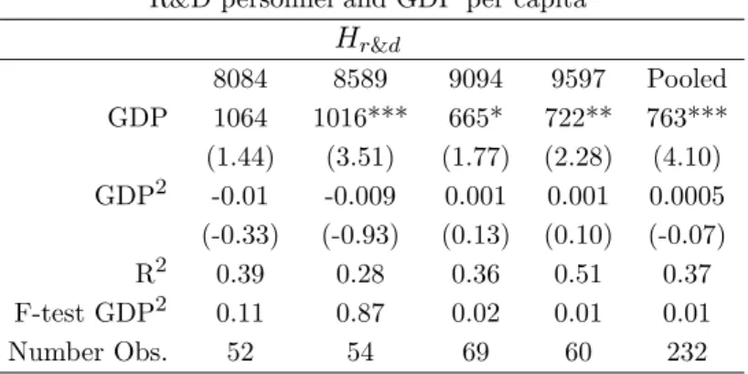
However, it can be shown that the proportion of R&D personnel and the level of GDP are closely related, as the next table supports. In fact, Scientists and Engineers employed in R&D (as a proportion of the total population) seems to have a positive relationship with the level of development as has been shown by Jones (1995a, b). Fact 2 makes the point.
Fact 2 - “R&D personnel” is positively correlated with GDP per capita.
on white-consistent variance-covariance matrix, except for the case of Least Absolute Deviations (LAD). The total number of observations is 621 and the number of outliers is 29. The number of countries in each cross-section is around 100. All the results in Table 1 could be obtained using LAD estimators, which accounts for the possible influence of outliers in the dependent variable and for possible non-normality on data.
Table 2 - Fact 2: The relationship between R&D personnel and GDP per capita
Hr&d 8084 8589 9094 9597 Pooled GDP 1064 1016*** 665* 722** 763*** (1.44) (3.51) (1.77) (2.28) (4.10) GDP2 -0.01 -0.009 0.001 0.001 0.0005 (-0.33) (-0.93) (0.13) (0.10) (-0.07) R2 0.39 0.28 0.36 0.51 0.37 F-test GDP2 0.11 0.87 0.02 0.01 0.01 Number Obs. 52 54 69 60 232
Sources: WDI. Calculations by the authors.
1.1.2 Some evidence of structural transformation and convergence
One of the most striking features of the human evolution in the two last centuries is the massive reallocation of labor and production from agriculture into industry and services. This is a very recent phenomenon which began with the Industrial Revolution. Table 3 shows the results of Rebelo et al. (2001). This shows that phases of economic growth and structural dynamics are closely related.
Table 3 - Fact 3: Structural transformation
Share of Employment Share of consumption
Agriculture declines declines
Manufacturing stable stable
Services increases increases
Source: Rebelo et al. (2001).
Fact 3 summarizes the result.
Fact 3 - More developed countries tend to have larger shares of the service sector and small shares of the agriculture sector. Middle-income countries tend to have the greatest industrial shares.
Data from the Statistical abstract and from the Historical Statistics of the United States, show clear evidence of increasing growth rates of Services employment when compared to growth rates of Manufacturing employment, after 1890 (Ruttan, 2002: figure 2). Also the
British industrial output presented higher growth than did services output in the early industrial times, but the output from the services sector grew at higher pace in the devel-oped world (Crafts, 1995; Crafts and Harley, 1992). Hereinafter, we will call the changes in quantities produced by different sectors in the economy across the different stages of development “Fact 3 in quantities”.
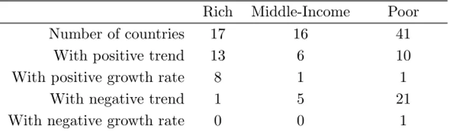
Rebelo et al. (2001) also pointed out that services prices increase with the USA’s development. We extended the analysis for all countries for which we had data. In the next table we show that more developed countries tend to have higher and consistent growth rates of the services prices.5 We calculated the services prices using services value added
at constant and current prices and GDP at constant and current prices. We calculated the price of services with reference to GDP price. We then calculated trends on the evolution of the services prices series and its growth rate year by year, to account for the persistence of price movements. Table 4 summarizes the results.
Table 4 - Fact 4: services prices dynamics
Rich Middle-Income Poor
Number of countries 17 16 41
With positive trend 13 6 10
With positive growth rate 8 1 1
With negative trend 1 5 21
With negative growth rate 0 0 1
Notes: Trends and Growth rates are significant at the 10% level. Sources: WDI. Calculations by the authors.
Fact 4 - In the richest countries, services prices are consistently increasing, while in poorer countries they do not show a consistent tendency.
In fact, 81% of the rich countries show an increasing trend of services prices and for 50% of them, this is persistent. These proportions fall to 35% and 6%, respectively, in middle-income countries and to 24% and 2% in poor countries. In these last two groups,
5For that, we have divided countries into three groups: rich (above 10000 USD), middle-income (between
2000 and 10000 USD) and poor (below 2000 USD). For the first group, we select those countries with values for 1980 onwards and for the other two groups those which have values for 1970 on. This was necessary in order to have more observations on the group of the rich countries.
more than 95% of the 58 countries show no significant persistence in prices movements. Fact 4 summarizes the argument.
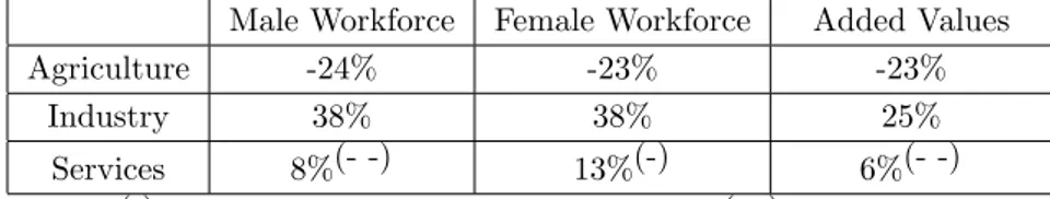
More technical graduates (engineering, applied mathematics, computer science) tend to be employed in industrial sectors but more low-tech graduates (law, social sciences, literature and humanities) tend to be employed in the services sector. This link between human capital composition and sectoral composition can be seen in data shown in Table 5. The Table shows correlations between high-low-tech ratio and workforce (columns 1 and 2) and added values in industry and services (column 3). This evidence is summarized in Fact 5 and will be an assumption in our model.
Table 5 - Fact 5: Correlations between high-low-tech ratio and Sector shares Male Workforce Female Workforce Added Values
Agriculture -24% -23% -23%
Industry 38% 38% 25%
Services 8%(- -) 13%(-) 6%(- -)
Note: (-) means significant at the 5% level and (- -) at the 20% level. No sign means significant at the 1% level.
Source: Unesco Database and World Development Indicators. Calculations by the authors.
Fact 5 - Technical graduates are mainly employed in the industrial sector and low-tech ones are mainly employed in the services sector.
A great number of empirical studies have detected significant conditional convergence when the regression includes controls for human capital, with Barro (1991) and Barro and Sala-i-Martin (1992, 1995) being the more significative.6 There is also time series evidence,
supported by Maddison (1995, 2001), that developed countries after 1910 have slowed down their rate of growth when compared to the period between 1870 and 1910 eventhough “the
6In practice we may observe that some middle-income countries in the fifties and sixties grew faster than
the more developed ones between that period and the nineties, with Japan, Portugal, Spain, South Korea being mere examples of this when compared with United States, United Kingdom or France. Thus, some authors, and most recently Easterly and Levine (1997), have modelled growth as a quadratic function of initial income. A common finding is that middle income countries have grown faster once controlling for policy differences.
pace of technological advance was substantially faster in the twentieth century than in the nineteenth” (Maddison, 2001, p.101).
Fact 6 - In general, growth regressions show strong evidence of conditional con-vergence.
2
The Benchmark Model
We consider an economy with an industrial sector, a services sector and an R&D sector. Also, there is accumulation of physical capital and of two types of human capital, high and low-tech human capital.
2.1 The accumulation of human capital
The existing stocks of high-tech and low-tech human capital are denoted by H and L. Accumulation of each type of human capital uses its own type with a CRS technology. However, there is a crucial difference between the two types of human capital: productivity in the accumulation of high-tech human capital decreases with the rate of technological development. This acts as an endogenous depreciation mechanism and formalizes the idea that high-tech human capital has to be up to date with the latest technologies. Thus, the accumulation of the two types of human capital is given by:
· H = γHH(1 − δ · n n), γ, δ > 0 (1) · L = ξLL, ξ > 0 (2)
where nn· represents the rate of technological development in this economy given by the rate of growth of the number of varieties of intermediate goods. The parameter δ on equation (1) reflects the impact on the accumulation of H of technological progress, when it occurs.7
7The functionH = γH·
H−δ
·
n
nH, γ, δ > 0 was also tested without any qualitative changes and only slightly
quantitative ones. The parcel δn·
With this structure for human capital accumulation, we assume that Research and Development has two different and opposite effects on productivity and growth: (1) a positive and direct effect on economic growth and (2) a negative and indirect effect on growth, due to high-tech human capital depreciation. It also has two different and opposite effects on human capital: (1) the level of technological knowledge increases human capital productivity in its market employments but (2) the rate of technological change decreases productivity in the accumulation of high-tech human capital.
2.2 Technology
Production of the homogenous final good Y uses physical capital, services and an index of intermediate goods. The latter is represented by the usual Dixit and Stiglitz formulation:
D = ·Z n 0 xαidi ¸1/α , 0 < α < 1 (3) where n denotes the number of available varieties, xi is the input of intermediate good i and
α controls the elasticity of substitution between varieties, which is equal to 1/(1 − α) > 1.
Intermediate goods are produced only with high-tech human capital and services S, are produced with a combination of high-tech and low-tech human capital. This is a simple way of introducing the notion that the industrial sector is more high-tech intensive than the services sector,
xi= Hxi (4)
S = LθSHS1−θ, with 0<θ<1 (5)
The final good (Y), which we take as numeraire, is produced with a Cobb-Douglas technology:
Y = A1K1−η−ψDηSψ, η, ψ > 0 (6)
Consumption goods, C, and investment goods, K, are all produced with the same technol-·
ogy. For simplicity, we neglect depreciation of physical capital, which leads to the economy’s resource constraint,
Y = C +K· (7)
Production of a new intermediate good requires the invention of a new blueprint. For emphasis of the following exposure, we assume that the production of new ideas is solely determined by the aggregate knowledge employed in R&D which is determined by high-tech human capital employed in R&D labs:8
·
n = ²Hn, ² > 0 (8)
2.3 Households
The population size is normalized to one, so all aggregate magnitudes can be interpreted as
per capita quantities. Human capital is supplied inelastically.9 Therefore, full employment
requires that,
H = HS+ HH + Hn+ Hx (9)
L = LS+ LL. (10)
where Hx is total high-tech human capital used in the production of intermediate goods.
Households earn wages, wH and wL, per unit of each type of employed human capital
(H − HH) and (L − LL).10 They also earn returns, r, per unit of aggregate wealth, A,
8Consideration of only High-tech human capital in the R&D technology is only a matter of simplification,
which do not have any influence on our results. Consideration of a more complex technology with spillovers
·
n = ²Hnnφ(like in Jones (1995b)) would introduce small changes to the conclusions. This is considered,
together with market power in services when we calibrate the model.
9We do not consider the choice of becoming high or low-tech. High-tech do not perform low-tech tasks,
as in equilibrium wH= wL+ κt, with κt > 0. Sequeira (2003b) addresses this issue.
10We look at the representative household which has both H and L. Also, this does not necessarily mean
that human capital used in the accumulation of human capital is not paid in the market. Simple modifications would account for this, assuming that the wage at schools may be a proportion of wage at the sectors Y and
which leads to a budget constraint A = rA + w· H(H − HH) + wL(L − LL) − C. Subject
to this constraint and the knowledge formation technologies (1) and (2) they maximize intertemporal utility Ut =
R∞
t log(Ct)e−ρ(τ −t)dτ , where ρ > 0 denotes the time preference
rate. Private agents take the aggregate rate of innovation as given. Using the control variables C > 0, HH ≥ 0 and LL≥ 0 we obtain from the first order conditions,
· C C = r − ρ (11) HH > 0 and · wH wH = r − γ(1 − δ · n n) or HH = 0 (12) LL> 0 and · wL wL = r − ξ or LL= 0 (13)
The first of these equations is the standard Ramsey rule. The second and third indicate that the growth rate of wages must be sufficiently high compared to the interest rate to ensure investment in human capital. The condition for high-tech human capital wage was obtained assuming that agents take the rate of innovation as a constant. This is verified in equilibrium and implies that the growth rate of high-tech wage is constant.
2.4 Firms and Markets
The markets for the final good and its inputs are perfectly competitive. This implies that:
r = (1 − η − ψ) Y K , (14) pD = ηYD, (15) pS= ψY S , (16)
where pD represents the price index for intermediates and pS the price of services. Each
firm in the industrial sector owns an infinite patent for selling its variety xi. Producers act
under monopolistic competition and maximize operating profits
πi= (pi− wH)xi, (17)
where pxi denotes the price of an intermediate and wH is the unit cost of xi. The demand
for each intermediate good results from the maximization of profits.11 Profit maximization
in the intermediate goods sector implies that each firm charges a price of,
pi = p = wH/α. (18)
With identical technologies and symmetric demand, the quantity supplied is the same for all goods, xi = x. Hence, equation (3) can be written as,
D = n1/αx. (19)
From pDD = pxn together with equations (15) and (18) we obtain the total quantity of
intermediates produced at each period and so, the value of Hx,
X = xn = Hx= αηYw
H . (20)
After insertion of equations (20) and (18) into (17), profits can be rewritten as a function of aggregate individual output and the number of existing firms:
π = (1 − α)ηY /n. (21)
Let υ denote the value of an innovation, defined by
vt= Z ∞ t e−[R(τ )−R(t)]π(τ )dτ , where R(τ ) = Z t 0 r(τ )dτ (22)
Taking into account the cost of an innovation as determined by eq.(8) , free-entry in R&D
implies that,
wH/² = υ and n > 0 (H. n> 0) (23)
wH/² > υ and n = 0. (Hn= 0) (24)
Finally, no-arbitrage requires that investing in R&D has the same return as investing in physical capital:
·
υ
υ = r − π/υ. (25)
From (25) we conclude that ππ. = υυ. for a stable growth rate of υ. With equations (3)-(25) the economy is fully described. In the following section we will describe the general equilibrium of this theoretical economy and show how it may describe stylized facts shown in section 1. We look at the steady-state solution for two different stages of development and at the transition between them. Before we proceed with the analysis we compute some equations that will be useful for calculating the steady-state. From the insertion of Eqs. (19) and (20) into production function (6), we reach the condensed form of that function:
Y1−η= A2K1−η−ψnη
1−α
α Sψ
wηH where A2= A1(αη)
η (26)
At the steady-state the shares of factor of production in each sector must be constant. Hence, each of the allocations of H must grow at the same rate as the total stock and the same applies to L. Thus, from (5) we obtain gS = θgL+ (1 − θ)gH and its dual. With (16)
we obtain that,
gpS = θgwL+ (1 − θ)gwH = gY − θgL− (1 − θ)gH. (27)
Using growth rates provided by log-differentiation of (20) in (27) we obtain that, at the steady-state,
3
Stages of development
3.1 The first stage of development
We look at a first stage of development in which the economy invests in high and low-tech human capital but not on R&D.12. So, we begin with a situation in which w
H > ²υ,n = 0.
and Hn= 0.13
At the steady-state the rate of growth of consumption is constant, implying that con-sumption, output and capital grow at constant and equal rates. Taking this into account, and using (7) - from which gY = gC, in the steady-state, (11) to (13), (20) and (28), and
the fact that at the steady-state the share of H in each utilization is constant, we obtain that in this stage steady-state the growth rates of human capital stocks are given by,
gH = γ − ρ (29)
and
gL= ξ − ρ (30)
The High-low-tech human capital ratio, defined by H/L, increases in this stage of de-velopment if γ > ξ. This is what we see in the data for less developed economies, so we look at this case (see Fact 1).
From (26), with (5), (20) and (28), we obtain that:
(1 − η)gY = (1 − η − ψ) (gK) + ψ [(1 − θ)(gY − gwH) + θ(gY − gwL)] − ηgwH. (31)
Taking into account that at the steady-state output, capital and consumption grow at the same rate we obtain gY.
gY = [ψ(1 − θ) + η] (γ − ρ) + θψ(ξ − ρ)
ψ + η (32)
12We could define a previous stage of development where there is only investment in physical capital: this
would be a Ramsey type economy. This changes nothing to our proposes.
13We could look at a transitory phase where g
H> gL= 0, but that would not change our results. It could
Proposition 1 At the steady-state of stage 1, the growth rate of consumption and
pro-duction is a weighted average of the growth rates of H and L and decreases with the time preference factor (ρ). The growth rate of wages increases with the productivity of the other type of human capital and decreases with its own productivity.
Proof. Taking (7) and (11) into account we obtain the steady state value of r. Inserting
r in (12) and (13), we can also obtain the growth rates of wL and wH This is summarized
as: r = [ψ(1 − θ) + η] γ + θψξ ψ + η (33) gwH = r − γ = ψθ [ξ − γ] ψ + η , (34) gwL = r − ξ = [ψ(1 − θ) + η] (γ − ξ) ψ + η . (35)
The differentiated-goods-sector share (η) has a positive effect and the services-sector-share (ψ) has a negative effect in the economy growth rate if and only if γ > ξ. The intuition behind the negative effect of the share of the services sector in the economy growth rate is based on the allocation of high-tech human capital between this sector and the intermediate goods sector.14 We can also see that, for γ > ξ high-tech human capital grows at higher
rates than does GDP per capita, and GDP grows at higher rates than does low-tech human capital, while wH decreases and wL increases. Under the same condition the growth rate of
industrial output (gX) is greater than the growth rate of the services output (gS) - Fact 3.
3.2 Transition between stages of development
The steady-state of stage 1 is only a transitory equilibrium, as in Funke and Strulik (2000) or in Sφrensen (1999). While there is no R&D the growth rate of profits is growing with output.
14Had we considered that intermediate goods are produced with final product Y or a combination of the
two stocks of human capital with the same share θ of the services technology, r∗would still be a weighted
average of productivity in human capital accumulation: (1 − θ)γ + θξ. In this case, the effects of the sectors’ shares on growth rates would turn out to be zero.
This also means that, profits on existing varieties grow faster than the cost of inventing a new one. Then, at some point it is worth to invest in R&D. The next proposition shows that in equilibrium, there are incentives to shift from the first stage to the second. We look at transitional dynamics and convergence features in appendix.
Proposition 2 If individuals invest in high-tech human capital (which happens if γ > ρ),
then the economy will invest in R&D at some period in time.
Proof. At the steady-state r is constant and, from (22), v may be calculated as vt=
πt/(ρ + gn). For gn= 0 and (21), this implies that gυ= gπ = gY . So, for γ > ρ, gv > gwH.
This implies that, though initially wH > ²υ, at some period in time we must have that
wH = ²υ.
This also means that, while there is no R&D, profits on existing varieties grow faster than the cost of inventing a new one. Then, at some point it is worth to invest in R&D. Note that investment in human capital is a necessary and sufficient condition to enter into an R&D stage. The following theorem makes the point.
Theorem 1 Investment in human capital is a necessary and sufficient condition to enter
into an R&D stage.
Proof. On necessity: If gH=0, gwH=gY=gυ, so if we begin with wH > ²υ, this will
remain in effect unless gH>0 implying that gwH<gv.
On sufficiency: The last proposition showed sufficiency.
Thus, we will now consider a last stage of development where there is investment in R&D.
3.3 The second stage of development
We now determine the growth rate of the economy in the steady-state of the last stage of development. This last stage is characterized by the existence of R&D. From (8), to obtain
a constant innovation rate in the steady-state we must have gn= gH. Conditions (11), (12)
and (20) imply that gH = γ(1 − δgn) − ρ. Thus, using the fact that gn= gH, we reach:
gH = 1 + δγγ − ρ (36)
For low tech human capital the condition is the same as before. We just rewrite it,
gL= ξ − ρ (37)
Proposition 3 With investment in R&D gL> gH in this stage if γ < 1−δ(ξ−ρ)ξ . So, H/L
increases in developing countries and decreases in developed ones (Fact 1) if and only if ξ < γ < 1−δ(ξ−ρ)ξ .
Proof. Eqs. (36) and (37) give the proof.
This proposition shows that the model can replicate Fact 1, presented in Section 1. Note that Fact 2 is also replicated in a very simple way, because when we arrive at the last stage in the model, there is an increase in Hn, which becomes positive.15
Taking into account that in the steady-state the shares of factors in each sector must be constant, (20) and (26) imply that,
gY = (1 − η − ψ) (gK) +1 − αα ηgH + ψ [(1 − θ)gH+ θgL] + ηgH (38)
Again, at the steady-state, the rate of growth of consumption is constant, implying that consumption, output and capital grow at constant and equal rates. Taking this into account and the rates of growth of H and L given in (36) and (37) we obtain the rate of growth of
15Note that in the model all the variables are per capita, which means that H
nis the model equivalent to
R&D personnel as a percent of total population in data. If the services’ price growth were zero in developed countries, it could be shown that the only solution consistent with an innovating economy is that gL> gH.
As it is only a theoretical hypothesis, as we have shown in section 1 that the growth rate of prices is positive in rich countries, we do not show the proof. It is available if requested.
output at this last stage of development,
gY = [η/α + ψ(1 − θ)]
γ−ρ
1+δγ + θψ(ξ − ρ)
η + ψ (39)
Proposition 4 a) With an active R&D sector, the growth rate of consumption and
pro-duction are positively enhanced by the monopolistic markup (1/α) and by the productivity of the human capital accumulation sector (γ and ξ).
b) Each growth rate of wages increases with the productivity in the accumulation of the other type of human capital. However, high-tech human capital benefits from its own productivity increase if and only if ψθ < 1−αα η.
Proof. From (11), (12), and (13), we can now obtain r and the growth rates of wL and
wH, r = [η/α + ψ(1 − θ)] γ−ρ 1+δγ + θψ(ξ − ρ) η + ψ + ρ, (40) gwH = r − γ(1 − δgn) = 1−α α η1+δγ1 (γ − ρ) ψ + η + ψθ(ξ − 1+δγγ (1 + δρ)) ψ + η , (41) gwL = r − ξ = 1−α α η1+δγ1 (γ − ρ) ψ + η − [ψ(1 − θ) + η] (ξ − 1+δγγ (1 + δρ)) ψ + η . (42)
The preference discount rate (ρ) has two opposite effects on the rate of growth: a positive effect evaluated at ((1−θ)ψψ+η + ψ+ηη )1+δγδγ , and a negative effect of −
1−α
α η1+δγ1
ψ+η − 1
which dominates. This happens because as individuals prefer present consumption, they will decrease innovation, which, besides the usual negative effect, now has a positive effect on the accumulation of high-tech human capital.
Note that it is possible to have a positive contribution of the industrial sector share to economic growth.16 It may be proved that ρ < 1−ααθ ρ+ξ
1−δ(ξ−ρ)+1−ααθ <
ξ
1−δ(ξ−ρ), which leads
16This is interesting because the influential article of Baumol (1967) and related literature discuss the
to the conclusion that it is possible to have the following results simultaneously: (1) high-tech human capital growing less than low-high-tech human capital and (2) industrial sector contributing more to economic growth than the services sector in the second stage. The intuition is that the higher the monopolies markups (1
α), the higher the impact of the
industrial sector on growth and the higher the innovation rate. But as the innovation rate increases, there is a negative effect on high-tech human capital accumulation. If this effect is strong enough, those two results may occur simultaneously.17
Under the condition defined in this last proposition, in the first stage gX > gS and in the second stage gX < gS, which links the evolution of human capital composition and the
increasing importance of the services sector in the economy. However, with a Cobb-Douglas specification, we must have constant shares of sectors. Thus, we look more carefully at this question in section 6. Next theorem summarizes the results obtained so far.
Theorem 2 Under the following conditions on parameters the model simultaneously
veri-fies Fact 1, Fact 2, Fact 4 (in quantities), Fact 5 and Fact 6. (i) ξ < γ < 1−δ(ξ−ρ)ξ .
(ii) 1−α
α η > [ηθ] δγ.
(iii) 1−αα η < [ψ(1 − θ) + η] δγ.
Proof. Fact 2 is always verified. Proposition 3 shows that condition (i) sustains Facts 1 and 3. Let xi, i = 1, 2 be the variable at stage i. Solving for gp2S > g1pS using (27) together with (34) and (35) for g1
pS and together with (41) and (42) for g
2
pS shows that condition
(ii) sustains Fact 4. Solving gY1 > g2Y using (32) and (39) shows that condition (iii) sustains Fact 6.18
relative costs of this sector. Our model has crucial different predictions because human capital is accumulable. Nevertheless, the services sector can still have a deterimental relative effect on economic growth.
17Had we considered that intermediate goods were produced with the final good or with a combination
of the two human capital stocks, the effect of the services sector would be clearly negative in the second stage. In these cases, equilibrium interest rate will be r∗= 1−αα η1+γ1 (γ−ρ)
ψ + ψh(1−θ) γ 1+γ(1+ρ)+θξ i ψ and r ∗= 1−α α η1+γ1 (γ−ρ) ψ+η + (ψ+η) h (1−θ)1+γγ (1+ρ)+θξ i ψ+η , respectively.
Thus, Facts 1 to 6 can be verified simultaneously. Verification of Fact 1, 3 and 6 depends on human capital technology. Simultaneous verification of Fact 4 and 6 depends on human capital technology and on the allocation of human capital between sectors.
We now determine the shares of H in each sector and obtain the equilibrium value for
H/n, which in the following section we compare to the optimal solutions. In this stage (23)
holds and then gwH = gυ. Hence, equation (25) may be written as
gwH = r − ²π/wH (43)
Inserting (16) in wH = (1−θ)pHSsS and then inserting the resulting equation for wH, (21)
and (41) into (43), we obtain the high-tech human capital share in services production:
uS= HS H = (1 − θ)ψ η 1 ² 1 (1 − α)γ 1 + δρ 1 + δγ n H (44)
Using the same steps than we have used to obtain uS, we can state that:
ux= 1 ² α 1 − αγ 1 + δρ 1 + δγ n H (45)
So, in equilibrium uS/ux= (1−θ)ψαη . From the varieties production function and the high-tech
human capital accumulation technology, using (36), we reach:
un= 1 ² n H γ − ρ (1 + δγ) (46) uH = γ − ρ γ(1 + δρ) (47)
Using (44) to (47) and the condition un+ uH+ ux+ uS= 1, we get to the competitive equilibrium level of H/n: H n = γ ²ρ · 1 + δρ 1 + δγ ¸2· γα 1 − α µ 1 +(1 − θ)ψ αη ¶ + γ − ρ (1 + δρ) ¸ (48)
4
Efficiency
To compare the competitive equilibrium outcome with the social optimum we only look at the last stage of development. Since the intermediate-goods sector is symmetric, the so-cial planner employs the quantity xi = x of each intermediate good. He maximizes Ut =
R∞
t log(Ct)e−ρ(τ −t)dτ , subject to the constraints .
K = Y −C, where Y = A2K(1−η−ψ)(n
1
α−1nx)ηSψ,
and the two human capital production technologies in (1) and (2). The control variables are C, Hn, Hs, Ls and x, and we take into account that Hx = nx. From the current value
Hamiltonian for this problem we obtain the first order conditions.
1/Ct= λ1 (49) λ4² = λ2γ(1 − δgn) + λ2δγ²HnH (50) λ1(1 − θ)ψY HS = λ2γ(1 − δgn) (51) λ1θψY LS = λ3ξ (52) λ1ηYx = nγ(1 − δgn)λ2 (53) λ1(1 − η − ψ)KY = ρλ1− · λ1 (54) λ2(γ(1 − δgn)) = ρλ2− · λ2 (55) λ3ξ = ρλ3− · λ3 (56) −xγ(1 − δgn)λ2+ λ1(η Y αn) + λ2δγHH² Hn n2 = ρλ4− · λ4 (57)
From insertion of (51) and (53) into the production function we obtain income per capita as Y = A2K1−η−ψ(n 1−α α )η[LS]θψ[HS](1−θ)ψ+η, where A2 = A1 · η (1 − θ)ψ ¸η (58) At the steady-state the rate of growth of consumption is constant, thus (52) and (56) imply that L/L = ξ − ρ, as in the competitive equilibrium. From (53) and (55) we obtain·
·
H/H = 1+δγγ−ρ, which is also given in the decentralized solution by (36) and is again equal to
·
that at the steady-state the shares of factors in each sector are constant we obtain the rate of growth of output at the optimum, gSP
Y ,
gYSP = [η/α + ψ(1 − θ)]
γ−ρ
1+δγ + θψ(ξ − ρ)
η + ψ (59)
Theorem 3 All growth rates in the economy are optimal.
Now we determine the efficient allocations of human capital between sectors. Insertion of λ1 from (51) in (57) after using (53), and consideration of (50) provides:
u∗S = 1 ² ψ(1 − θ) η α 1 − α · γ(1 + δρ) (1 + δγ) n H + δ²ρ (γ − ρ)(1 + δγ) γ(1 + δρ)2 ¸ (60) Insertion of λ2 from (53) in (57) and consideration of (50) provides,
u∗x= 1 ² α 1 − α · γ(1 + δρ) (1 + δγ) n H + δ²ρ (γ − ρ)(1 + δγ) γ(1 + δρ)2 ¸ (61)
So, in the optimum uS/ux = (1−θ)ψη , which is smaller than the equilibrium value for this
ratio. From the varieties production function and the high-tech human capital accumulation technology, we obtain: u∗n= 1 ² n H γ − ρ (1 + δγ) (62) u∗H = γ − ρ γ(1 + δρ) (63)
As u∗n+ u∗H + u∗x+ u∗S= 1, we can determine H/n in the social planner solution,
µ H n ¶∗ = γ ²ρ · 1 + δρ 1 + δγ ¸2 h γα 1−α ³ 1 +(1−θ)ψη ´ +(1+δρ)γ−ρ i 1 − δ α 1−α ³ 1 +(1−θ)ψη ´ (γ−ρ) (1+δρ) (64)
Comparing (48) to (64), it is easy to see that there are two opposite distortions between the decentralized and the social planner solution: (i) the monopoly markup, from which we tend to have higher H/n than optimal and (ii) the externality, from which we may have lower H/n than we should. If the first distortion dominates, we will get a lack of R&D when
compared to the high-tech human capital, u∗
n > un, u∗x > ux and u∗s < us. If, however, the
second distortion dominates we will get lower high-tech to varieties ratio in the steady-state than in the social planner solution, u∗
n < un, u∗x > ux and u∗s < us or u∗s > us. The share
of high-tech human capital in the education sector is optimal (u∗
H = uH), as this does not
depend on H/n.
Theorem 4 The competitive equilibrium allocates less high-tech human capital to the
indus-trial sector than would the social planner. Other allocations of H depend on which distortion dominates. The allocation of L between services and human capital accumulation is optimal.
Proof. For results on H compare (45) with (61), (44) with (60), (46) with (62) and (47) with (63). For this, we have to consider a comparison between (48) and (64).
For the result on L, use the low-tech human capital accumulation in (2) to have LL L = ·
L/L
ξ . The proof is concluded verifying that the growth rate of low-tech human capital in the
decentralized equilibrium is equal to the social planner one.
We make two remarks on these results. The first is that this externality is a new reason to get over-production of ideas. The second is to note that, even though there is an increasing concern about the lack of engineering and technical knowledge in developed countries, this concern may be misleading. In fact, our model suggests that we may have not a level problem, but an allocation problem. This consists, notably, of a lack of high-tech skills in industry and, depending on which is the stronger distortion, an over or under allocation of high-tech skills both in R&D and in services. An incentive policy to the consumption of intermediate goods may be Pareto-improving, solving the markup distortion. Policies such as taxes on R&D or subsides to high-tech accumulations, which are natural candidates to solve the externality distortion, fail to do so. The first one only affect the free-entry condition in R&D, increasing the cost of a new ideia and has not growth effects, as Arnold (1998) has shown. It can also be shown that the second, although changes the high-tech human capital growth rate, introduces new distortions in the economy.19
19A subside like this changes the household resource constraint to a = ra + w(H − (1 − s)H·
H − C)
and introduces new distortions in uH. For reasonable values of parameters ux/us fall in the competitive
5
Calibration Procedure
In this section, we quantitatively test the model. We calibrate the model presented in the previous section and also an extension that considers spillovers in R&D and market power in services, as this may be relevant for quantitative results. We follow Funke and Strulik (2000) and Jones and Williams (2000) in doing this calibration. We depart from the method used by the first authors in a crucial point: we calibrate the model for the first stage and then determine the range of parameters for which our facts are plausible to occur in the second stage. We then assess the quantitative importance of the distortion implied by the depreciation externality.
We calibrate the model for the United States of America. We consider that this country entered the second stage between 1870 and 1890, when the US “second industrial revolution” began. This has been supported, for instance, by Maddison (2001). We compare a period in the first stage (1850-1870) to a recent period (1973-1986) to have a clear distinction between stages’ “steady-states”. In the first period the average GDP per capita growth rate is 1.44% and in the second period is 1.49%, according to Maddison (1995).20.
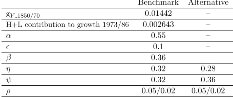
We need values for the shares in the economy, β, ψ, η, and θ, the elasticity of substitution between varieties (α), the productivity of the R&D sector (²) and the average annual growth rate of GDP per capita (gY) in the first stage. The share of capital is assumed as 0.36 and R&D productivity is 0.1, as is usual in economic growth literature.21 For industrial and
services shares we initially assume equal values. In fact, Maddison (1995) showed that both in 1820 and in 1870, the USA showed very similar shares for these two sectors (15% in 1820 and 26% in 1870, for each sector). We also state the results of a calibration where a higher services share is imposed (ψ = 0.36). For the elasticity of substitution between varieties we assumed the value of 0.55. This is in line with values used by Jones and
20We picked GDP per capita growth rates for the whole economy from Maddison (1995) to be consistent
between two stages. Ideally we should have used GDP growth rates in the non-education sector, as in Jorgenson and Fraumeni (1993), but no sources are available for this figures in the first stage and for countries other than the USA. For the USA between 1973 and 1986, the growth rate in the non-education sector is 1.85% but for the whole economy, as showed by Maddison is 1.49%. Our procedure is under the assumption that differences between growth rates for the whole economy and for the non-education sector are equal in both stages.
Williams (2000) (α = 0.5572, implying a markup of 1.37) and Funke and Strulik (2000), who used α = 0.54. We used two alternative values of ρ, 0.05 and 0.02.22 We assumed the
value for the share of low-tech human capital in the services sector, θ, to be 0.7, using the assumption and evidence of low-tech intensity in this sector. Variations in this parameter from 0.5 to 0.9 have not crucial importance in our results. In the first stage we calculate the growth rate of both types of human capital so that (1) the given growth rate of GDP
per capita is fulfilled, (2) the growth rate of high-tech human capital is higher than the
growth rate of low-tech human capital.23 Of course we get a range of possible pairs (ξ, γ)
that satisfy these conditions. Human capital contribution to growth in the second stage is from Jorgenson and Fraumeni (1993, p.16), using their measure of labor quality. High-tech human capital growth rate is obtained in the second-stage steady-state using the shares from the calibration assumptions and values for ξ and γ that come from the first stage. In this procedure we differ from Funke and Strulik (2000), whose departure point is the growth rate of TFP (that in the model steady-state is proportional to the high-tech human capital growth rate). We consider that our approach is cleaner from measurement errors linked with different forms of growth accountings and with other production factors (such as physical capital) construction. Finally, we analyze the fit of the model comparing actual to predicted growth rate.
These calibrations are conducted assuming that countries in the first stage are in the steady-state, before investing in R&D
Next table summarizes the values for calibration.
22These are in the range of values used in all of the literature cited.
23We also assume that both human capital growth rates are positive or null. Such a condition for H is
Table 6 - Calibration Benchmark Alternative gY 1850/70 0.01442 – H+L contribution to growth 1973/86 0.002643 – α 0.55 – ² 0.1 – β 0.36 – η 0.32 0.28 ψ 0.32 0.36 ρ 0.05/0.02 0.05/0.02
This exercise is more general than it could appear. As an example, it could also be applied to a comparison between South America - as a country in the first stage - and the United States - as a country in the second stage - in the second half of the tweentieth century, as this set of countries presented an average growth rate of 1.47%, quite similar to that of the USA in the first stage. Applying such an exercise to countries with greater differences in economic growth between stages (such as South Asia - 3.27% - and USA after 1950, for instance) would increase the predicted depreciation rate.
5.1 Calibration Results for the Benchmark Model
With the discount rate (ρ) and the productivity of the low-tech human capital in low-tech accumulation sector (ξ), we calculate the high-tech human capital productivity (γ), so that we reach two conditions in the first stage: (1) the given growth rate of GDP per capita equal to 0.01442, (2) a higher growth rate of high-tech human capital than the growth rate of low-tech human capital. The next table shows the ranges of ξ and γ that fit these conditions for the two alternative values of ρ.
Table 7 - Productivity of high-tech accumulation for given values of ξ and ρ Benchmark Alternative
A B C D
min ξ γ max ξ γ min ξ γ max ξ γ ρ = 0.05 0.051 0.072 0.061 0.066 0.051 0.073 0.060 0.067
Note: The minimum ξ is the smallest that ensures a positive growth rate of L and a maximum ξ is the highest that ensures that gH > gLin the second stage.
For the next stage, we only need the contribution of human capital for growth, (η + (1 − θ)ψ)gH+ ψθgL, which is 0.2643%, from Jorgenson and Fraumeni (1993). We can then
calculate the coefficient of depreciation, δ, and the depreciation rate, δgn. The following
tables present these values.
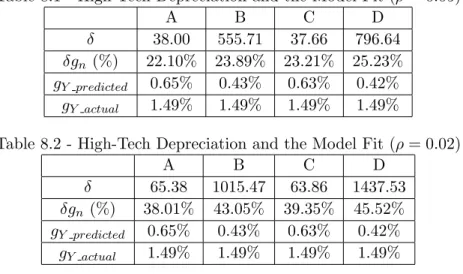
Table 8.1 - High-Tech Depreciation and the Model Fit (ρ = 0.05)
A B C D
δ 38.00 555.71 37.66 796.64
δgn (%) 22.10% 23.89% 23.21% 25.23%
gY predicted 0.65% 0.43% 0.63% 0.42%
gY actual 1.49% 1.49% 1.49% 1.49%
Table 8.2 - High-Tech Depreciation and the Model Fit (ρ = 0.02)
A B C D
δ 65.38 1015.47 63.86 1437.53
δgn(%) 38.01% 43.05% 39.35% 45.52%
gY predicted 0.65% 0.43% 0.63% 0.42%
gY actual 1.49% 1.49% 1.49% 1.49%
The depreciation rate implied by this mechanism seems to be high and stable across different modifications of parameter values that fulfil the conditions stated above, presenting values from near 20% (for the high discount rate case) to near 40% (for the low discount rate case). However, predicted growth rates of per capita output are far from the actual.
We can now assess the range of parameter ξ for which Facts 1, 3, 4 and 6 are verified. We also state conclusions for an additional fact: a positive effect of the industry share in the first and second stages. The next tables show results for calibrations with the two different values for the discount rate.
Table 9: Values ofξ for which the cited Facts are verified Benchmark Alternative ρ = 0.05 ρ = 0.02 ρ = 0.05 ρ = 0.02 Fact 1 [0.055, 0.061] [0.025, 0.034] [0.055, 0.060] [0.025, 0.030] Fact 3 [0.055, 0.061] [0.025, 0.034] [0.055, 0.060] [0.025, 0.030] Fact 4 φ φ φ φ Fact 6 [0.051, 0.061] [0.021, 0.031] [0.051, 0.060] [0.021, 0.030] Additional Fact [0.051, 0.056] [0.021, 0.026] [0.051, 0.056] [0.021, 0.026]
Note: Limits of intervals are rounded to three decimal points. The additional fact stands for a positive ∂gY
∂η , which means a positive effect of the industry share on growth.
All facts, but Fact 4, can occur simultaneously. It is also worth noting that intervals for verification of Facts 1 and 3 represent more than 60% of the whole interval that fulfill the two conditions stated above. However, in this case Fact 6 should not occur as the USA did increase its growth rate. This happens due to poor performance of the model in replicating growth rates. Tables 8 and 9 also show that changes in calibration in sectoral shares change almost nothing in the predicted depreciation rate and in the length of the verification intervals. Even differences in the discount rate have only a levels effect in the intervals length. From then on, we leave the alternative calibration and concentrate on the benchmark one with the high and low discount rates.
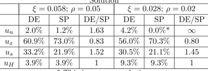
Next we can calculate the H/n ratio and the equilibrium and optimal allocations of H between sectors, when Fact 1 holds. We choose the mean point of intervals for Fact 1 (0.058 and 0.028, respectively) in the previous table. If this is the case, with both discount rates considered and the benchmark values, high-tech workers would have a 1% higher growth rate than low-tech in the first stage, but 0.6% lower in the second stage. The depreciation rate is 23.3% in the high discount rate case and 41.2% in the low discount rate case.
Table 10 - Comparison between the Decentralized Equilibrium and the Social Planner Solution ξ = 0.058; ρ = 0.05 ξ = 0.028; ρ = 0.02 DE SP DE/SP DE SP DE/SP un 2.0% 1.2% 1.63 4.2% 0.0%* ∞ ux 60.9% 73.0% 0.83 56.0% 70.3% 0.80 us 33.2% 21.9% 1.52 30.5% 21.1% 1.45 uH 3.9% 3.9% 1 9.3% 9.3% 1
* This is a corner solution.
The introduction of the externality effect cause serious overinvestment in R&D, as well as significant distortions in industry and services.24 We obtain that the joint effect of the
externality and the markup differential cause over-allocation of engineers to services and under-allocation to the industrial sector. In fact, the social planner would allocate nearly 12% more of engineers to industry and nearly 11% less to services.
As the main problem of this exercise is a lower predicted GDP growth rate than the actual one we will now the actual growth rate in the second stage keeping the value for ξ at the mean point of the intervals found in Table 9. We iterate the contribution of total human capital so that we get a GDP growth rate of 1.49%. The reached value was (η + (1 −
θ)ψ)gH + ψθgL =0.6545%, much higher than the one given by empirical estimations.The
model fitness is evaluated according to the replication of empirical facts (Except for Fact 6, that is now our objective). For the high discount rate case (ξ = 0.058; ρ = 0.05) we get a depreciation rate of 9.51%. For the low discount rate case (ξ = 0.028; ρ = 0.02) we get a depreciation rate of 17.0%. For both cases we cannot replicate the first two facts, although Fact 4 and the Additional Fact can be verified. Data on replication of empirical facts 1 and 3 are presented in the following table.
24If the unique distortion was the markup the equilibrium allocation to industry would be optimal. If the
unique distortion was the externality, it would account for 0.42% of mis-allocation (overinvestment in R&D and under-investment in Industry and Services).
Table 11 - Replication of Main Facts with the actual growth rate of GDP Stage 1 Stage 2
Fact 1: gH − gL 0.99% 0.34%
Fact 3: gX − gS 0.69% 0.24%
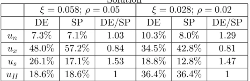
This shows that with this higher contribution of human capital to growth, it is impossible for this model to replicate Facts 1 and 3 for the USA. Next, we present the comparison between the decentralized and the social equilibrium in this case.
Table 12 - Comparison between the Decentralized Equilibrium and the Social Planner Solution ξ = 0.058; ρ = 0.05 ξ = 0.028; ρ = 0.02 DE SP DE/SP DE SP DE/SP un 7.3% 7.1% 1.03 10.3% 8.0% 1.29 ux 48.0% 57.2% 0.84 34.5% 42.8% 0.81 us 26.1% 17.1% 1.53 18.8% 12.8% 1.47 uH 18.6% 18.6% 1 36.4% 36.4% 1
We get now pretty higher shares of high-tech human capital allocated to R&D and Human capital accumulation. In consequence, the social planner would allocate more 8% to 11% of high-techs to industry and less 6% to 10% to the services sector. Investment in R&D is almost optimal in the high discount rate case and there are some over-investment in the low discount rate case.
5.2 Calibration with spillovers in R&D and market power in services
This section presents results for calibration, when we consider a model that generalizes the previous setting, introducing a non-competitive framework in the services sector and spillovers in R&D activities. We show that this setting improves the model fitness to reality. In fact, both empirical and theorectical literature point out the existence of spillovers and it is also reasonable to expect some degree of monopoly power in the services sector. Also this allows us to isolate the influence of the depreciation externality, introducing the same degree of monopoly power in the services sector than in industry.
The specification for R&D technology is borrowed from Jones (1995b), not considering the duplication externality,
.
n = Hnnφ (65)
The technology in the services sector now considers a differentiated-goods setup,
S = ·Z m 0 sϕidi ¸1/ϕ (66) where m is the number of firms in the sector. Each s is produced with the same combination of high and low-tech human capital as we had before for total S, but producers act under monopolistic competition, maximizing operating profits,
πsi = (psi− ΘwLθw
1−θ
H )si, (67)
where psi denotes the price of an intermediate and ΘwθLw1−θH is the unit cost of each s, with
Θ = θ−θ(1 − θ)θ−1. Facing elasticity of demand ε
s= 1/(1 − ϕ) each firm charges a price,
psi = ΘwθLwH1−θ/ϕ. (68)
Free entry in this sector implies that firms enter the market until the present value of profits becomes equal to the cost of installing the firm, which we assume to be fixed at F units of Y . So,
F = ω for
·
m
m > 0 (69)
where ω is the present value of future profits in the sector. Again, a non-arbitrage condition may be written as rω = πs+ω. All the equations for the other sectors in the·
economy are equal to those in Sections 2 and 3 for the benchmark model. In the appendix we develop the expressions that we apply to this case and that based our calibration exercise. For the calibration, we assume a spillover of 0.4, which is nearly half of the values sug-gested and used in the literature (see Jones, 1995b or Jones and Williams, 2000). However,
recent empirical work which include human capital reveal an important role for this fac-tor and much more smaller values for national and international spillovers than have been reported before - domestic spillovers in the presence of human capital decrease near 55% when compared to the model without human capital (Barrio-Castro et al., 2002).25 Values
for spillovers in this range do not change our results. As empirical evidence on the different degrees of monopoly power across sectors is not easily obtained, we set a markup in the services sector equal to that in the industrial sector (ϕ = 0.55). This allows us to isolate the effect of the depreciation externality and to compare it with the spillovers effect.
Also note that the depreciation rate is calculated in order to fit the growth rate of n, that is proportional to the high-tech human capital growth rate. We present values for the benchmark calibration and for both values of the discount rate previously considered.
The following table presents values for depreciation rate and a comparison between predicted and effective growth rate of GDP per capita.
Table 13 - High-tech depreciation and Model Fit
ρ = 0.05 A B δ 22.80 333.43 δgn (%) 22.10% 23.89% gY predicted 1.37% 0.75% gY actual 1.49% 1.49% ρ = 0.02 A B δ 39.23 609.28 δgn (%) 38.01% 43.66% gY predicted 1.37% 0.75% gY actual 1.49% 1.49%
Values in the table above show that the presence of spillovers and the markup in the services sector do not crucially change depreciation rates, that remain between 20% and 40%, but increase the predicted GDP growth rate that remain slightly below the actual value. Now, we determine the range of values of ξ for which the refered facts are fitted under this new specification.
Table 14 - Values of ξ for which the cited Facts are verified Benchmark ρ = 0.05 ρ = 0.02 Fact 1 [0.055, 0.061] [0.025, 0.031] Fact 3 [0.055, 0.061] [0.025, 0.031] Fact 4 [0.051, 0.057] [0.021, 0.027] Fact 6 [0.051, 0.061] [0.024, 0.031]
Note: Limits of intervals are rounded to three decimal points.
So, the presence of spillovers and the end of the monopoly distortion leads to a greater set of values for all facts are verified. We again present a comparison between the decentralized equilibrium and the social planner solution for this generalized model, using the same middle point for the first interval in Table 14.
Table 15 - Comparison between the Decentralized Equilibrium and the Social Planner Solution ξ = 0.058; ρ = 0.05 ξ = 0.028; ρ = 0.02 DE SP DE/SP DE SP DE/SP un 3.7% 2.7% 1.37 7.6% 2.5% 3.00 ux 71.0% 71.8% 0.99 63.9% 67.8% 0.94 us 21.3% 21.5% 0.99 19.2% 20.4% 0.94 uH 3.9% 3.9% 1 9.3% 9.3% 1
This extension makes it possible to avoid the markup distortion, which results in an equal relative distortion in Services and Industry sectors and again in over-investment in R&D. As growth rates are still slightly below the actual one, we proceed as before to target this growth rate. The reached value for the human capital contribution was (η + (1 −
θ)ψ)gH+ ψθgL=0.36676%. All facts (1,3 and 4) are fulfilled and we get depreciation rates
of 20% and 35% in the high and low discount rates cases, respectively. Next table presents data on the replication of Facts 1 and 3.
Table 16 - Replication of Main Facts with the actual growth rate of GDP Stage 1 Stage 2
Fact 1: gH − gL 0.99% -0.35%
In the next table we finally compare decentralized and social equilibrium in the case that we target the growth rate of GDP.
Table 17 - Comparison between the Decentralized Equilibrium and the Social Planner Solution ξ = 0.058; ρ = 0.05 ξ = 0.028; ρ = 0.02 DE SP DE/SP DE SP DE/SP un 6.9% 5.6% 1.24 11.9% 6.3% 1.89 ux 65.2% 66.2% 0.98 53.6% 57.9% 0.93 us 19.6% 19.9% 0.98 16.1% 17.4% 0.93 uH 8.3% 8.3% 1 18.4% 18.4% 1
This exercise is quite interesting because it shows that accounting for the actual growth rate of GDP, the model can account for different levels of distortions. However, over-investment in R&D are still predicted (with lower levels).26 We then see that the new
externality rivalize with spillovers in the allocation of high-tech talent to R&D or to Industry and Services. Again, this approximation to the actual GDP growth rate brings up the shares in the R&D and in the human capital accumulation sectors.
The main difference between this setting (with spillovers and without monopoly distor-tion) and the previous one is that the relative distortion between industry and services ends with the end of the monopoly distortion.
The overall conclusions of these calibration exercises are the following
(1) quite reasonable depreciation rates of high-tech human capital due to R&D are ob-tained, from 9% up to 49% (with the alternative functionH = γH· H−δ
· n
nH the depreciation
rate is between 0.6% and 1.6%;
(2) facts 1 to 6 are verified for relevant intervals of parameter values;
(3) the model easily accounts for under and over-investment in R&D, which depend crucially on the relationship between the externality and the spillover in a setting with no monopoly distortions;
26Only with φ = 0.7 (for the high discount rate case) and φ = 0.8 (for the low discount rate case), the

![Table 9: Values of ξ for which the cited Facts are verified Benchmark Alternative ρ = 0.05 ρ = 0.02 ρ = 0.05 ρ = 0.02 Fact 1 [0.055, 0.061] [0.025, 0.034] [0.055, 0.060] [0.025, 0.030] Fact 3 [0.055, 0.061] [0.025, 0.034] [0.055, 0.060] [0.025, 0.030] Fact](https://thumb-eu.123doks.com/thumbv2/123dok_br/15131693.1010861/29.892.197.760.211.364/table-values-cited-facts-verified-benchmark-alternative-fact.webp)