EUROPEAN ORGANISATION FOR NUCLEAR RESEARCH (CERN)
JHEP 10 (2018) 047
DOI:10.1007/JHEP10(2018)047
CERN-EP-2017-161 18th October 2018
Angular analysis of
B
0
d
→ K
∗
µ
+
µ
−
decays in
p p
collisions at
√
s
= 8 TeV with the ATLAS detector
The ATLAS Collaboration
An angular analysis of the decay B0d → K∗µ+µ− is presented, based on proton–proton collision data recorded by the ATLAS experiment at the LHC. The study is using 20.3 fb−1 of integrated luminosity collected during 2012 at centre-of-mass energy of
√
s = 8 TeV. Measurements of the K∗ longitudinal polarisation fraction and a set of angular parameters obtained for this decay are presented. The results are compatible with the Standard Model predictions.
1 Introduction
Flavour-changing neutral currents (FCNC) have played a significant role in the construction of the Standard Model of particle physics (SM). These processes are forbidden at tree level and can proceed only via loops, hence are rare. An important set of FCNC processes involve the transition of a b-quark to an sµ+µ−final state mediated by electroweak box and penguin diagrams. If heavy new particles exist, they may contribute to FCNC decay amplitudes, affecting the measurement of observables related to the decay under study. Hence FCNC processes allow searches for contributions from sources of physics beyond the SM (hereafter referred to as new physics). This analysis focuses on the decay B0d → K∗0(892)µ+µ−, where K∗0(892) → K+π−. Hereafter, the K∗0(892) is referred to as K∗and charge conjugation is implied throughout, unless stated otherwise. In addition to angular observables such as the forward-backward asymmetry AFB1, there is considerable interest in measurements of the charge asymmetry, differential
branching fraction, isospin asymmetry, and ratio of rates of decay into dimuon and dielectron final states, all as a function of the invariant mass squared of the dilepton system q2. All of these observable sets can be sensitive to different types of new physics that allow for FCNCs at tree or loop level. The BaBar, Belle, CDF, CMS, and LHCb collaborations have published the results of studies of the angular distributions for B0
d → K
∗µ+µ−
[1–8]. The LHCb Collaboration has reported a potential hint, at the level of 3.4 standard deviations, of a deviation from SM calculations [3,4] in this decay mode when using a parameterization of the angular distribution designed to minimise uncertainties from hadronic form factors. Measurements using this approach were also reported by the Belle and CMS Collaborations [6,8] and they are consistent with the LHCb experiment’s results and with the SM calculations. This paper presents results following the methodology outlined in Ref. [3] and the convention adopted by the LHCb Collaboration for the definition of angular observables described in Ref. [9]. The results obtained here are compared with theoretical predictions that use the form factors computed in Ref. [10].
This article presents the results of an angular analysis of the decay B0d → K∗µ+µ− with the ATLAS detector, using 20.3 fb−1 of pp collision data at a centre-of-mass energy
√
s = 8 TeV delivered by the Large Hadron Collider (LHC) [11] during 2012. Results are presented in six different bins of q2 in the range 0.04 to 6.0 GeV2, where three of these bins overlap. Backgrounds, including a radiative tail from B0
d → K
∗
J/ψ events, increase for q2 above 6.0 GeV2, and for this reason, data above this value are not
studied.
The operator product expansion used to describe the decay Bd0 → K∗µ+µ− encodes short-distance contributions in terms of Wilson coefficients and long-distance contributions in terms of operators [12]. Global fits for Wilson coefficients have been performed using measurements of Bd0 → K∗µ+µ−and other rare processes. Such studies aim to connect deviations from the SM predictions in several processes to
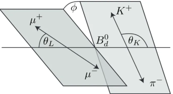
centre-of-mass frame (θK); the angle between the µ+and the direction opposite to the Bd0 in the dimuon centre-of-mass frame (θL); and the angle between the two decay planes formed by the K π and the dimuon systems in the B0d rest frame (φ). For B0dmesons the definitions are given with respect to the negatively
charged particles. Figure1illustrates the angles used.
φ
B
d0µ
+µ
−K
+π
−θ
Lθ
KFigure 1: An illustration of the Bd0 → K∗µ+µ−decay showing the angles θK, θLand φ defined in the text. Angles are computed in the rest frame of the K∗, dimuon system and Bd0 meson, respectively.
The angular differential decay rate for Bd0 → K∗µ+µ−is a function of q2, cos θK, cos θL and φ, and can be written in several ways [16]. The form to express the differential decay amplitude as a function of the angular parameters uses coefficients that may be represented by the helicity or transversity amplitudes [17] and is written as2 1 dΓ/dq2 d4Γ d cos θLd cos θKdφdq2 = 9 32π " 3(1 − FL) 4 sin 2θ K + FLcos2θK+ 1 − FL 4 sin 2θ Kcos 2θL
−FLcos2θKcos 2θL + S3sin2θKsin2θLcos 2φ
+S4sin 2θKsin 2θLcos φ + S5sin 2θKsin θLcos φ +S6sin2θKcos θL+ S7sin 2θKsin θLsin φ
+S8sin 2θKsin 2θLsin φ + S9sin2θKsin2θLsin 2φ #
. (1)
Here FL is the fraction of longitudinally polarised K∗mesons and the Siare angular coefficients. These angular parameters are functions of the real and imaginary parts of the transversity amplitudes of Bd0 decays into K∗µ+µ−. The forward-backward asymmetry is given by AFB = 3S6/4. The predictions for
the S parameters depend on hadronic form factors which have significant uncertainties at leading order. It is possible to reduce the theoretical uncertainty in these predictions by transforming the Si using ratios
P1 = 2S3 1 − FL (2) P2 = 2 3 AFB 1 − FL (3) P3 = − S9 1 − FL (4) Pj0=4,5,6,8 = pSi=4,5,7,8 FL(1 − FL) . (5)
All of the parameters introduced, FL, Si and P(0)j , may vary with q2and the data are analysed in q2bins to obtain an average value for a given parameter in that bin.
3 The ATLAS detector, data, and Monte Carlo samples
The ATLAS experiment at the LHC is a general-purpose detector with a cylindrical geometry and nearly 4π coverage in solid angle [19]. It consists of an inner detector (ID) for tracking, a calorimeter system and a muon spectrometer (MS). The ID consists of silicon pixel and strip detectors, with a straw-tube transition radiation tracker providing additional information for tracks passing through the central region of the detector.3 The ID has a coverage of |η| < 2.5, and is immersed in a 2T axial magnetic field generated by a superconducting solenoid. The calorimeter system, consisting of liquid argon and scintillator-tile sampling calorimeter subsystems, surrounds the ID. The outermost part of the detector is the MS, which employs several detector technologies in order to provide muon identification and a muon trigger. A toroidal magnet system is embedded in the MS. The ID, calorimeter system and MS have full azimuthal coverage.
The data analysed here were recorded in 2012 during Run 1 of the LHC. The centre-of-mass energy of the pp system was
√
s= 8 TeV. After applying data-quality criteria, the data sample analysed corresponds to an integrated luminosity of 20.3 fb−1. A number of Monte Carlo (MC) signal and background event samples were generated, with b-hadron production in pp collisions simulated with Pythia 8.186 [20,21]. The AU2 set of tuned parameters [22] is used together with the CTEQ6L1 PDF set [23]. The EvtGen 1.2.0 program [24] is used for the properties of b- and c-hadron decays. The simulation included modelling of multiple interactions per pp bunch crossing in the LHC with Pythia soft QCD processes. The simulated events were then passed through the full ATLAS detector simulation program based on Geant 4 [25,26]
4 Event selection
Several trigger signatures constructed from the MS and ID inputs are selected based on availability during the data-taking period, prescale factor and efficiency for signal identification. Data are combined from 19 trigger chains where 21%, 89% or 5% of selected events pass one or more triggers with one, two, or at least three muons identified online in the MS, respectively. Of the events passing the requirement of at least two muons, the largest contribution comes from the chain requiring one muon with a transverse momentum pT > 4 GeV and the other muon with pT > 6 GeV. This combination of triggers ensures that
the analysis remains sensitive to events down to the kinematic threshold of q2 = 4m2µ, where mµ is the muon mass. The effective average trigger efficiency for selected signal events is about 29%, determined from signal MC simulation.
Muon track candidates are formed offline by combining information from both the ID and MS [27]. Tracks are required to satisfy |η| < 2.5. Candidate muon (kaon and pion) tracks in the ID are required to satisfy pT > 3.5 (0.5) GeV. Pairs of oppositely charged muons are required to originate from a common vertex with a fit quality χ2/NDF < 10.
Candidate K∗mesons are formed using pairs of oppositely charged kaon and pion candidates reconstructed from hits in the ID. Candidates are required to satisfy pT(K
∗) > 3.0 GeV. As the ATLAS detector does not
have a dedicated charged-particle identification system, candidates are reconstructed with both possible Kπ mass hypotheses. The selection implicitly relies on the kinematics of the reconstructed K∗meson to determine which of the two tracks corresponds to the kaon. If both candidates in an event satisfy selection criteria, they are retained and one of them is selected in the next step following a procedure described below. The K π invariant mass is required to lie in a window of twice the natural width around the nominal mass of 896 MeV, i.e. in the range [846, 946] MeV. The charge of the kaon candidate is used to assign the flavour of the reconstructed B0dcandidate.
The B0dcandidates are reconstructed from a K∗candidate and a pair of oppositely charged muons. The four-track vertex is fitted and required to satisfy χ2/NDF < 2 to suppress background. A significant amount of combinatorial, B0d, B+, B0s and Λb background contamination remains at this stage. Combinatorial background is suppressed by requiring a B0dcandidate lifetime significance τ/στ > 12.5, where the decay
time uncertainty στ is calculated from the covariance matrices associated with the four-track vertex fit and with the primary vertex fit. Background from final states partially reconstructed as B → µ+µ−X accumulates at invariant mass below the B0d mass and contributes to the signal region. It is suppressed by imposing an asymmetric mass cut around the nominal Bd0 mass, 5150 MeV < mK πµµ < 5700 MeV.
The high-mass sideband is retained, as the parameter values for the combinatorial background shapes are extracted from the fit to data described in Section5. To further suppress background, it is required that the angle Θ, defined between the vector from the primary vertex to the B0dcandidate decay vertex and the B0
dcandidate momentum, satisfies cos Θ > 0.999. Resolution effects on cos θK, cos θL and φ were found
candidate reconstructed with the smallest value of |mK π− mK∗|/σ(mK π) is retained for analysis, where
mK π is the K∗candidate mass, σ(mK π) is the per-event uncertainty in this quantity, and mK∗ is the world
average value of the K∗mass.
The selection procedure results in an incorrect flavour tag (mistag) for some signal events. The mistag probability of a B0d (B0d) meson is denoted by ω (ω) and is determined from MC simulated events to be
0.1088 ± 0.0005 (0.1086 ± 0.0005). The mistag probability varies slightly with q2such that the difference ω − ω remains consistent with zero. Hence the average mistag rate hωi in a given q2bin is used to account
for this effect. If a candidate is mistagged, the values of cos θL, cos θK and φ change sign, while the latter two are also slightly shaped by the swapped hadron track mass hypothesis. Sign changes in these angles affect the overall sign of the terms multiplied by the coefficients S5, S6, S8and S9(similarly for the
corresponding P(0)parameters) in Equation (1). The corollary is that mistagged events result in a dilution factor of (1 − 2hωi) for the affected coefficients.
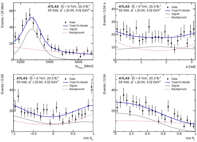
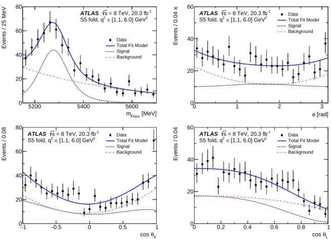
The region q2 ∈ [0.98, 1.1] GeV2 is vetoed to remove any potential contamination from the φ(1020) resonance. The remaining data with q2 ∈ [0.04, 6.0] GeV2 are analysed in order to extract the signal parameters of interest. Two K∗cc control regions are defined for B0d decays into K∗J/ψ and K∗ψ(2S), respectively as q2 ∈ [8, 11] and [12, 15] GeV2. The control samples are used to extract values for nuisance parameters describing the signal probability density function (pdf) from data as discussed in Section5.3. For q2 < 6 GeV2 the selected data sample consists of 787 events and is composed of signal B0d → K∗µ+µ− decay events as well as background that is dominated by a combinatorial component that does not peak in mK πµµ and does not exhibit a resonant structure in q2. Other background contributions are considered when estimating systematic uncertainties. Above 6 GeV2 the background contribution increases significantly, including events coming from B0d → K∗J/ψ with a radiative J/ψ → µ+µ−γ decay. Scalar K π contributions are neglected in the nominal fit and considered only when addressing systematic uncertainties. The data are analysed in the q2bins [0.04, 2.0], [2.0, 4.0] and [4.0, 6.0] GeV2, where the bin width is chosen to provide a sample of signal events sufficient to perform an angular analysis. The width is much larger than the q2resolution obtained from MC simulated signal events and observed in data for B0d decays into K∗J/ψ and K∗ψ(2S). Additional overlapping bins [0.04, 4.0], [1.1, 6.0] and [0.04, 6.0] GeV2
are analysed in order to facilitate comparison with results of other experiments and with theoretical predictions.
(Section5.1), treatment of background (Section5.2), use of K∗cc decay control samples (Section 5.3), fitting procedure and validation (Section5.4).
5.1 Signal model
The signal mass distribution is modelled by a Gaussian distribution with the width given by the per-event uncertainty in the K π µµ mass, σ(mK πµµ), as estimated from the track fit, multiplied by a unit-less scale
factor ξ, i.e. the width given by ξ · σ(mK πµµ). The mean values of the B0dcandidate mass (m0) and ξ of
the signal Gaussian pdf are determined from fits to data in the control regions as described in Section5.3. The simultaneous extraction of all coefficients using the full angular distribution of Equation (1) requires a certain minimum signal yield and signal purity to avoid a pathological fit behaviour. A significant fraction of fits to ensembles of simulated pseudo-experiments do not converge using the full distribution. This is mitigated using trigonometric transformations to fold certain angular distributions and thereby simplify Equation (1) such that only three parameters are extracted in one fit: FL, S3and one of the other S
parameters. For these folding schemes the angular parameters of interest, denoted by bp in Equation (6), are (FL, S3, Si) where i = 4, 5, 7, 8. These translate into (FL, P1, P
0
j), where j = 4, 5, 6, 8, using Equation (5).
Following Ref. [3], the transformations listed below are used:
FL, S3, S4, P0 4: φ → −φ for φ < 0 φ → π − φ for θL > π2 θL →π − θL for θL > π2, (7) FL, S3, S5, P 0 5: (φ → −φ for φ < 0 θL →π − θL for θL > π2, (8) FL, S3, S7, P0 6: φ → π − φ for φ > π2 φ → −π − φ for φ < −π 2 θL →π − θL for θL > π2, (9) FL, S3, S8, P 0 8: φ → π − φ for φ > π2 φ → −π − φ for φ < −π2 θL →π − θL for θL > π2 θK →π − θK for θL > π2. (10)
the data. The values and uncertainties of FL and S3obtained from the four fits are consistent with each
other and the results reported are those found to have the smallest systematic uncertainty.
Three MC samples are used to study the signal reconstruction and acceptance. Two of them follow the SM prediction for the decay angle distributions taken from Ref. [29], with separate samples generated for B0d and B0d decays. The third MC sample has FL = 1/3 and the angular distributions are generated
uniformly in cos θK, cos θL and φ. The samples are used to study the effect of potential mistagging and reconstruction differences between particle and antiparticle decays and for determination of the acceptance. The acceptance function is defined as the ratio of reconstructed and generated distributions of cos θK, cos θL, φ, i.e. it is compensating for the bias in the angular distributions resulting from triggering, reconstruction and selection of events. It is described by sixth-order (second-order) polynomial distributions for cos θKand cos θL (φ) and is assumed to factorise for each angular distribution, i.e. using ε(cos θK, cos θL, φ) = ε(cos θK)ε(cos θL)ε(φ). A systematic uncertainty is assessed in order to account
for this assumption. The acceptance function multiplies the angular distribution in the fit, i.e. the signal pdf is
Pkl = ε(cos θK)ε(cos θL)ε(φ)g(cos θK, cos θL, φ) · G(mK πµµ),
where g(cos θK, cos θL, φ) is an angular differential decay rate resulting from one of the four folding
schemes applied to Equation (1) and G(mK πµµ) is the signal mass distribution. The MC sample generated
with uniform cos θK, cos θL and φ distributions is used to determine the nominal acceptance functions for each of the transformed variables defined in Equations (7)–(10). The other samples are used to estimate the related systematic uncertainty. Among the angular variables the cos θL distribution is the most affected by the acceptance. This is a result of the minimum transverse momentum requirements on the muons in the trigger and the larger inefficiency to reconstruct low-momentum muons, such that large values of | cos θL| are inaccessible at low q2. As q2 increases, the acceptance effects become less severe. The cos θK distribution is affected by the ability to reconstruct the K π system, but that effect shows no significant variation with q2. There is no significant acceptance effect for φ. Figure2 shows the acceptance functions used for cos θK and cos θL for two different q2 ranges for the nominal angular distribution given in Equation (1).
0.4 0.5 0.6 0.7 2 [0.04, 2.0] GeV ∈ 2 q 2 [4.0, 6.0] GeV ∈ 2 q 0.8 1 1.2 q2∈ [0.04, 2.0] GeV2 2 [4.0, 6.0] GeV ∈ 2 q
5.2 Background modes
The fit to data includes a combinatorial background component that does not peak in the mK πµµ distribu-tion. It is assumed that the background pdf factorises into a product of one-dimensional terms. The mass distribution of this component is described by an exponential function and second-order Chebychev poly-nomials are used to model the cos θK, cos θL and φ distributions. The values of the nuisance parameters describing these shapes are obtained from fits to the data independently for each q2bin.
Inclusive samples of bb → µ+µ−X and cc → µ+µ−X decays and eleven exclusive B0d, B0s, B+ and Λb
background samples are studied in order to identify contributions of interest to be included in the fit model, or to be considered when estimating systematic uncertainties. The relevant exclusive modes found to be of interest are discussed below. Events with Bcdecays are suppressed by excluding the q2range containing the J/ψ and ψ(2S), and by charm meson vetoes discussed in Section 7. The exclusive background decays considered for the signal mode are Λb→ Λ(1520)µ+µ−, Λb → pK−µ+µ−, B+→ K(∗)+µ+µ−and B0
s → φµ+µ −
. These background contributions are accounted for as systematic uncertainties estimated as described in Section7.
Two distinct background contributions not considered above are observed in the cos θK and cos θL
distributions. They are not accounted for in the nominal fit to data, and are treated as systematic effects. A peak is found in the cos θKdistribution near 1.0 and appears to have contributions from at least two distinct sources. One of these arises from misreconstructed B+ decays, such as B+ → K+µµ and B+ →π+µµ. These decays can be reconstructed as signal if another track is combined with the hadron to form a K∗ candidate in such a way that the event passes the reconstruction and selection. The second contribution comes from combinations of two charged tracks that pass the selection and are reconstructed as a K∗ candidate. These fake K∗candidates accumulate around cos θK of 1.0 and are observed in the K π mass sidebands away from the K∗meson. They are distinct from the structure of expected S-, P- and D-wave Kπ decays resulting from a signal B0
d→ Kπµµ transition. The origin of this source of background is not
fully understood. The observed excess may arise from a statistical fluctuation, an unknown background process, or a combination of both. Systematic uncertainties are assigned to evaluate the effect of these two background contributions, as described in Section7.
Another peak is found in the cos θL distribution near values of ±0.7. It is associated with partially reconstructed B decays into final states with a charm meson. This is studied using Monte Carlo simulated events for the decays D0→ K−π+, D+→ K−π+π+and D+s → K+K−π+. Events with a B meson decaying
via an intermediate charm meson D0, D+or D+s are found to pass the selection and are reconstructed in
such a way that they accumulate around 0.7 in | cos θL|. These are removed from the data sample when
estimating systematic uncertainties, as described in Section7.
is evaluated by allowing for 0, 1, 2 and 3 exclusive background components. The control sample fit projections for the variant of the fit including all three exclusive backgrounds can be found in Figure3. The impact of the used exclusive background model on the peak position and scale factor of the signal pdf is negligible. From these fits the statistical and systematic uncertainties in the values of m0 and ξ
are extracted for the B0d component in order to be used in the B0d → K∗µ+µ−fits. From the J/ψ control data it is determined that the values for the nuisance parameters describing the signal model pdf in the Kπµµ mass are m0 = 5276.6 ± 0.3 ± 0.4 MeV and ξ = 1.210 ± 0.004 ± 0.002, where the uncertainties are statistical and systematic, respectively. The ψ(2S) sample yields compatible results albeit with larger uncertainties. These results are similar to those obtained from the MC simulated samples, and the numbers derived from the K∗J/ψ data are used for the signal region fits.
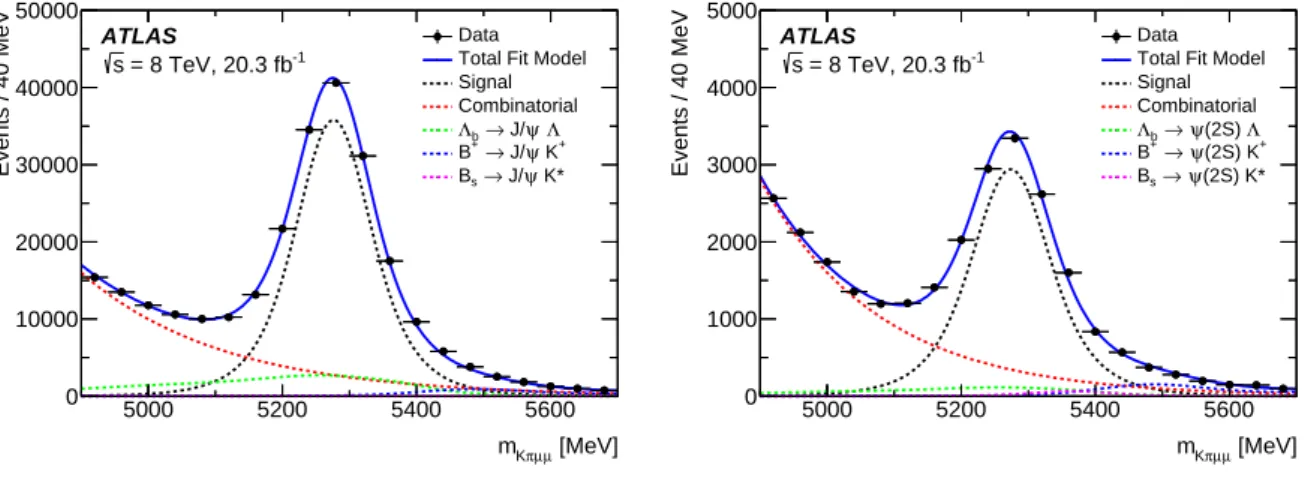
[MeV] µ µ π K m 5000 5200 5400 5600 Events / 40 MeV 0 10000 20000 30000 40000 50000 ATLAS -1 = 8 TeV, 20.3 fb s Data Total Fit Model Signal Combinatorial Λ ψ J/ → b Λ + K ψ J/ → + B K* ψ J/ → s B [MeV] µ µ π K m 5000 5200 5400 5600 Events / 40 MeV 0 1000 2000 3000 4000 5000 ATLAS -1 = 8 TeV, 20.3 fb s Data Total Fit Model Signal Combinatorial Λ (2S) ψ → b Λ + (2S) K ψ → + B (2S) K* ψ → s B
Figure 3: Fits to the K π µµ invariant mass distributions for the (left) K∗J/ψ and (right) K∗ψ(2S) control region samples. The data are shown as points and the total fit model as the solid lines. The dashed lines represent (black) signal, (red) combinatorial background, (green) Λb background, (blue) B+ background and (magenta) B0s
background components.
5.4 Fitting procedure and validation
A two-step fit process is performed for the different signal bins in q2. The first step is a fit to the K π µ+µ− invariant mass distribution, using the event-by-event uncertainty in the reconstructed mass as a conditional variable. For this fit, the parameters m0and ξ are fixed to the values obtained from fits to data control
injected into samples of background events generated from the likelihood. The signal yield determined from the first step in the fit process is found to be unbiased. The angular parameters extracted from the nominal fits have biases with magnitudes ranging between 0.01 and 0.04, depending on the fit variation and q2bin. A similar procedure is used to estimate the effect of neglecting S-wave contamination in the data sample. Neglecting the S-wave component in the fit model results in a bias between 0.00 and 0.02 in the angular parameters. Similarly, neglecting exclusive background contributions from Λb, B+and Bs0
decays that peak in mK πµµnear the B0dmass results in a bias of less than 0.01 on the angular parameters. All these effects are included in the systematic uncertainties described in section7. The P(0)parameters are obtained using the fit results and covariance matrices from the second fit along with Equations (2)–(5).
6 Results
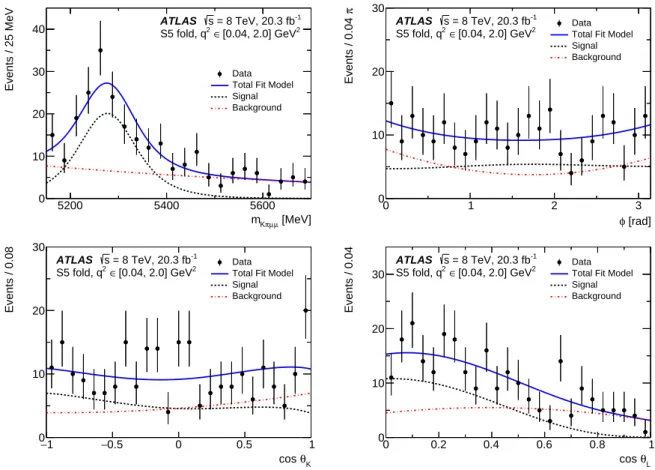
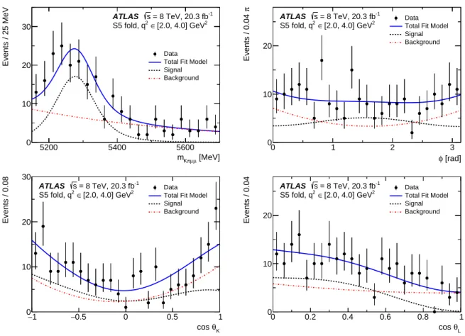
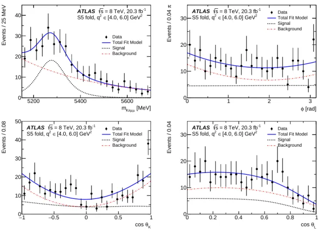
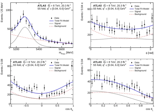
The event yields obtained from the fits are summarised in Table1where only statistical uncertainties are reported. Figures4through9show for the different q2 bins the distributions of the variables used in the fit for the S5folding scheme (corresponding to the transformation of Equation (8)) with the total, signal
and background fitted pdfs superimposed. Similar sets of distributions are obtained for the three other folding schemes: S4, S7and S8. The results of the angular fits to the data in terms of the Siand P
(0) j can be
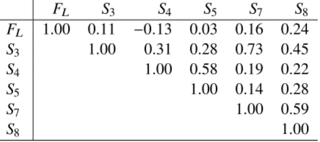
found in Tables2and3. Statistical and systematic uncertainties are quoted in the tables. The distributions of FL and the Si parameters as a function of q2are shown in Figure 10and those for P(0)j are shown in Figure11. The correlations between FL and the Siparameters and between FL and the P(0)j are given in AppendixA.
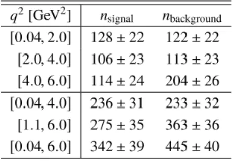
Table 1: The values of fitted signal, nsignal, and background, nbackground, yields obtained for different bins in q2. The
uncertainties indicated are statistical.
q2[GeV2 ] nsignal nbackground [0.04, 2.0] 128 ± 22 122 ± 22 [2.0, 4.0] 106 ± 23 113 ± 23 [4.0, 6.0] 114 ± 24 204 ± 26 [0.04, 4.0] 236 ± 31 233 ± 32 [1.1, 6.0] 275 ± 35 363 ± 36 [0.04, 6.0] 342 ± 39 445 ± 40
[MeV] µ µ π K m 5200 5400 5600 Events / 25 MeV 0 10 20 30 40 -1 = 8 TeV, 20.3 fb s ATLAS 2 [0.04, 2.0] GeV ∈ 2 S5 fold, q Data Total Fit Model Signal Background [rad] φ 0 1 2 3 Events / 0.04 0 10 20 -1 = 8 TeV, 20.3 fb s ATLAS 2 [0.04, 2.0] GeV ∈ 2 S5 fold, q Data Total Fit Model Signal Background K θ cos 1 − −0.5 0 0.5 1 Events / 0.08 0 10 20 30 -1 = 8 TeV, 20.3 fb s ATLAS 2 [0.04, 2.0] GeV ∈ 2 S5 fold, q Data Total Fit Model Signal Background L θ cos 0 0.2 0.4 0.6 0.8 1 Events / 0.04 0 10 20 30 -1 = 8 TeV, 20.3 fb s ATLAS 2 [0.04, 2.0] GeV ∈ 2 S5 fold, q Data Total Fit Model Signal Background
Figure 4: The distributions of (top left) mK πµµ, (top right) φ, (bottom left) cos θK, and (bottom right) cos θLobtained for q2 ∈ [0.04, 2.0] GeV2. The (blue) solid line is a projection of the total pdf, the (red) dot-dashed line represents
[MeV] µ µ π K m 5200 5400 5600 Events / 25 MeV 0 10 20 30 -1 = 8 TeV, 20.3 fb s ATLAS 2 [2.0, 4.0] GeV ∈ 2 S5 fold, q Data Total Fit Model Signal Background [rad] φ 0 1 2 3 π Events / 0.04 0 10 20 -1 = 8 TeV, 20.3 fb s ATLAS 2 [2.0, 4.0] GeV ∈ 2 S5 fold, q Data Total Fit Model Signal Background K θ cos 1 − −0.5 0 0.5 1 Events / 0.08 0 10 20 30 -1 = 8 TeV, 20.3 fb s ATLAS 2 [2.0, 4.0] GeV ∈ 2 S5 fold, q Data Total Fit Model Signal Background L θ cos 0 0.2 0.4 0.6 0.8 1 Events / 0.04 0 10 20 -1 = 8 TeV, 20.3 fb s ATLAS 2 [2.0, 4.0] GeV ∈ 2 S5 fold, q Data Total Fit Model Signal Background
Figure 5: The distributions of (top left) mK πµµ, (top right) φ, (bottom left) cos θK, and (bottom right) cos θLobtained for q2 ∈ [2.0, 4.0] GeV2. The (blue) solid line is a projection of the total pdf, the (red) dot-dashed line represents the background, and the (black) dashed line represents the signal component. These plots are obtained from a fit using the S5folding scheme.
[MeV] µ µ π K m 5200 5400 5600 Events / 25 MeV 0 10 20 30 40 -1 = 8 TeV, 20.3 fb s ATLAS 2 [4.0, 6.0] GeV ∈ 2 S5 fold, q Data Total Fit Model Signal Background [rad] φ 0 1 2 3 Events / 0.04 0 10 20 30 -1 = 8 TeV, 20.3 fb s ATLAS 2 [4.0, 6.0] GeV ∈ 2 S5 fold, q Data Total Fit Model Signal Background K θ cos 1 − −0.5 0 0.5 1 Events / 0.08 0 10 20 30 40 50 -1 = 8 TeV, 20.3 fb s ATLAS 2 [4.0, 6.0] GeV ∈ 2 S5 fold, q Data Total Fit Model Signal Background L θ cos 0 0.2 0.4 0.6 0.8 1 Events / 0.04 0 10 20 30 -1 = 8 TeV, 20.3 fb s ATLAS 2 [4.0, 6.0] GeV ∈ 2 S5 fold, q Data Total Fit Model Signal Background
Figure 6: The distributions of (top left) mK πµµ, (top right) φ, (bottom left) cos θK, and (bottom right) cos θLobtained for q2 ∈ [4.0, 6.0] GeV2. The (blue) solid line is a projection of the total pdf, the (red) dot-dashed line represents
[MeV] µ µ π K m 5200 5400 5600 Events / 25 MeV 0 20 40 60 -1 = 8 TeV, 20.3 fb s ATLAS 2 [0.04, 4.0] GeV ∈ 2 S5 fold, q Data Total Fit Model Signal Background [rad] φ 0 1 2 3 π Events / 0.04 0 10 20 30 40 -1 = 8 TeV, 20.3 fb s ATLAS 2 [0.04, 4.0] GeV ∈ 2 S5 fold, q Data Total Fit Model Signal Background K θ cos 1 − −0.5 0 0.5 1 Events / 0.08 0 20 40 -1 = 8 TeV, 20.3 fb s ATLAS 2 [0.04, 4.0] GeV ∈ 2 S5 fold, q Data Total Fit Model Signal Background L θ cos 0 0.2 0.4 0.6 0.8 1 Events / 0.04 0 20 40 -1 = 8 TeV, 20.3 fb s ATLAS 2 [0.04, 4.0] GeV ∈ 2 S5 fold, q Data Total Fit Model Signal Background
Figure 7: The distributions of (top left) mK πµµ, (top right) φ, (bottom left) cos θK, and (bottom right) cos θLobtained for q2 ∈ [0.04, 4.0] GeV2. The (blue) solid line is a projection of the total pdf, the (red) dot-dashed line represents the background, and the (black) dashed line represents the signal component. These plots are obtained from a fit using the S5folding scheme.
[MeV] µ µ π K m 5200 5400 5600 Events / 25 MeV 0 20 40 60 -1 = 8 TeV, 20.3 fb s ATLAS 2 [1.1, 6.0] GeV ∈ 2 S5 fold, q Data Total Fit Model Signal Background [rad] φ 0 1 2 3 Events / 0.04 0 20 40 -1 = 8 TeV, 20.3 fb s ATLAS 2 [1.1, 6.0] GeV ∈ 2 S5 fold, q Data Total Fit Model Signal Background K θ cos 1 − −0.5 0 0.5 1 Events / 0.08 0 20 40 60 80 -1 = 8 TeV, 20.3 fb s ATLAS 2 [1.1, 6.0] GeV ∈ 2 S5 fold, q Data Total Fit Model Signal Background L θ cos 0 0.2 0.4 0.6 0.8 1 Events / 0.04 0 20 40 60 -1 = 8 TeV, 20.3 fb s ATLAS 2 [1.1, 6.0] GeV ∈ 2 S5 fold, q Data Total Fit Model Signal Background
Figure 8: The distributions of (top left) mK πµµ, (top right) φ, (bottom left) cos θK, and (bottom right) cos θLobtained for q2 ∈ [1.1, 6.0] GeV2. The (blue) solid line is a projection of the total pdf, the (red) dot-dashed line represents
[MeV] µ µ π K m 5200 5400 5600 Events / 25 MeV 0 50 100 -1 = 8 TeV, 20.3 fb s ATLAS 2 [0.04, 6.0] GeV ∈ 2 S5 fold, q Data Total Fit Model Signal Background [rad] φ 0 1 2 3 π Events / 0.04 0 20 40 60 -1 = 8 TeV, 20.3 fb s ATLAS 2 [0.04, 6.0] GeV ∈ 2 S5 fold, q Data Total Fit Model Signal Background K θ cos 1 − −0.5 0 0.5 1 Events / 0.08 0 20 40 60 80 -1 = 8 TeV, 20.3 fb s ATLAS 2 [0.04, 6.0] GeV ∈ 2 S5 fold, q Data Total Fit Model Signal Background L θ cos 0 0.2 0.4 0.6 0.8 1 Events / 0.04 0 20 40 60 80 -1 = 8 TeV, 20.3 fb s ATLAS 2 [0.04, 6.0] GeV ∈ 2 S5 fold, q Data Total Fit Model Signal Background
Figure 9: The distributions of (top left) mK πµµ, (top right) φ, (bottom left) cos θK, and (bottom right) cos θLobtained for q2 ∈ [0.04, 6.0] GeV2. The (blue) solid line is a projection of the total pdf, the (red) dot-dashed line represents the background, and the (black) dashed line represents the signal component. These plots are obtained from a fit using the S5folding scheme.
S4 , S5 , S7 and S8 parameters obtained for different bins in q 2. The uncer tainties indicated are statis tical and sy stematic, S3 S4 S5 S7 S8 − 0 .02 ± 0 .09 ± 0 .02 0 .15 ± 0 .20 ± 0 .10 0 .33 ± 0 .13 ± 0 .08 − 0 .09 ± 0 .10 ± 0 .02 − 0 .14 ± 0 .24 ± 0 .09 − 0 .15 ± 0 .10 ± 0 .07 − 0 .37 ± 0 .15 ± 0 .10 − 0 .16 ± 0 .15 ± 0 .06 0 .15 ± 0 .14 ± 0 .09 0 .52 ± 0 .20 ± 0 .19 0 .00 ± 0 .12 ± 0 .07 0 .32 ± 0 .16 ± 0 .09 0 .13 ± 0 .18 ± 0 .09 0 .03 ± 0 .13 ± 0 .07 − 0 .12 ± 0 .21 ± 0 .05 − 0 .05 ± 0 .06 ± 0 .04 − 0 .15 ± 0 .12 ± 0 .09 0 .16 ± 0 .10 ± 0 .05 0 .01 ± 0 .08 ± 0 .05 0 .19 ± 0 .16 ± 0 .12 − 0 .04 ± 0 .07 ± 0 .03 0 .03 ± 0 .11 ± 0 .07 0 .00 ± 0 .10 ± 0 .04 0 .02 ± 0 .08 ± 0 .06 0 .11 ± 0 .14 ± 0 .10 − 0 .04 ± 0 .06 ± 0 .03 0 .03 ± 0 .10 ± 0 .07 0 .14 ± 0 .09 ± 0 .03 0 .02 ± 0 .07 ± 0 .05 0 .07 ± 0 .13 ± 0 .09 and P 0parameters 8 obtained for different bins in q 2. The uncer tainties indicated are statis tical and sy stematic, respectiv el y P 1 P 0 4 P 0 5 P 0 6 P 0 8 0 .30 ± 0 .08 0 .31 ± 0 .40 ± 0 .20 0 .67 ± 0 .26 ± 0 .16 − 0 .18 ± 0 .21 ± 0 .04 − 0 .29 ± 0 .48 ± 0 .18 0 .51 ± 0 .34 − 0 .76 ± 0 .31 ± 0 .21 − 0 .33 ± 0 .31 ± 0 .13 0 .31 ± 0 .28 ± 0 .19 1 .07 ± 0 .41 ± 0 .39 0 .43 ± 0 .26 0 .64 ± 0 .33 ± 0 .18 0 .26 ± 0 .35 ± 0 .18 0 .06 ± 0 .27 ± 0 .13 − 0 .24 ± 0 .42 ± 0 .09 0 .26 ± 0 .16 − 0 .30 ± 0 .24 ± 0 .17 0 .32 ± 0 .21 ± 0 .11 0 .01 ± 0 .17 ± 0 .10 0 .38 ± 0 .33 ± 0 .24 0 .31 ± 0 .13 0 .05 ± 0 .22 ± 0 .14 0 .01 ± 0 .21 ± 0 .08 0 .03 ± 0 .17 ± 0 .12 0 .23 ± 0 .28 ± 0 .20 0 .23 ± 0 .10 0 .05 ± 0 .20 ± 0 .14 0 .27 ± 0 .19 ± 0 .06 0 .03 ± 0 .15 ± 0 .10 0 .14 ± 0 .27 ± 0 .17
7 Systematic uncertainties
Systematic uncertainties in the parameter values obtained from the angular analysis come from several sources. The methods for determining these uncertainties are based either on a comparison of nominal and modified fit results, or on observed fit biases in modified pseudo-experiments. The systematic uncertainties are symmetrised. The most significant ones are described in the following, in decreasing order of importance.
• A systematic uncertainty is assigned for the combinatorial K π (fake K∗) background peaking at cos θK values around 1.0 obtained by comparing results of the nominal fit to that where data above cos θK = 0.9 are excluded from the fit.
• A systematic uncertainty is derived to account for background arising from partially reconstructed B → D0/D+/D+
sX decays, that manifest in an accumulation of events at | cos θL| values around
0.7. Two-track or three-track combinations are formed from the signal candidate tracks, and are reconstructed assuming the pion or kaon mass hypothesis. A veto is then applied for events in which a track combination has a mass in a window of 30 MeV around the D0, D+ or D+s meson
mass. Similarly, a veto is implemented to reject B+ → K+µ+µ−and B+ → π+µ+µ− events that pass the event selection. Here B+candidates are reconstructed from one of the hadrons from the K∗ candidate and the muons in the signal candidate. Signal candidates that have a three-track mass within 50 MeV of the B+mass are excluded from the fit. A few percent of signal events are removed when applying these vetoes, with a corresponding effect on the acceptance distributions. The fit results obtained from the data samples with vetoes applied are compared to those obtained from the nominal fit and the change in each result is taken as the systematic uncertainty from these backgrounds. This systematic uncertainty dominates the measurement of FL at higher values of q2. • The combinatorial background pdf shape has an uncertainty arising from the choice of the model. For the mass distribution it is assumed that an exponential function model is adequate; however, for the angular variables the data are re-fitted using third-order Chebychev polynomials. The change from the nominal result is taken as the uncertainty from this source.
• The acceptance function is assumed to factorise into three separate components, for cos θK, cos θL
and φ. To validate this assumption, the signal simulated events are fitted with the acceptance function obtained from that same MC sample. Differences in the fit results from expectation are small and taken as the uncertainty resulting from this assumption.
• A systematic uncertainty is assigned for the angular pdf model for the background by comparing the nominal result to that with a reduced fit range of mK πµµ ∈ [5200, 5700] MeV, in particular to
account for possible residues of the partially reconstructed B-decays.
• The pT spectrum of Bd candidates observed in data is not accurately reproduced by the MC
simulation. This difference in the kinematics results in a slight modification of the acceptance functions. This is accounted for by reweighting signal MC simulated events to resemble the pT
spectrum found in data. The change in fitted parameter values obtained due to the reweighting is taken as the systematic uncertainty resulting from this difference.
• The signal decay mode is resonant K∗→ Kπ decay, but scalar contributions from non-resonant Kπ transitions may also exist. The LHCb Collaboration reported an S-wave contribution at the level of 5% of the signal [4, 30]. Ensembles of MC simulated events are fitted with 5% of the signal being drawn from an S-wave sample of events and the remaining 95% from signal. The observed change in fit bias is assigned as the systematic uncertainty from this source. Any variation in S-wave content as a function of q2would not significantly affect the results reported here.
• The values of the nuisance parameters of the fit model obtained from MC control samples and fits to the data mass distribution have associated uncertainties. These parameters include m0, ξ, the signal
and background yields, the shape parameter of the combinatorial background mass distribution, and the parameters of the signal acceptance functions. The uncertainty in the value of each of these parameters is varied independently in order to assess the effect on parameters of interest. This source of uncertainty has a small effect on the measurements reported here.
• Background from exclusive modes peaking in mK πµµ is neglected in the nominal fit. This may affect the fitted results and is accounted for by computing the fit bias obtained when embedding MC simulated samples of Λb → Λ(1520)µ+µ−, Λb → pK−µ+µ−, B+→ K(∗)+µ+µ−and B0s →φµ+µ−
into ensembles of pseudo-data generated from the fit model containing only combinatorial back-ground and signal components. The change in fit bias observed when adding exclusive backback-grounds is taken as the systematic error arising from neglecting those modes in the fit.
• The difference from nominal results obtained when fitting the B0d signal MC events with the acceptance function for B0d is taken as an upper limit of the systematic error resulting from event migration due to mistagging the Bd0flavour.
• The parameters S5and S8, as well as the respective P (0)
j parameters are affected by dilution and thus
have a multiplicative scaling applied to them. This dilution factor depends on the kinematics of the K∗decay and has a systematic uncertainty associated with it. The effect of data/MC differences in the pTspectrum of B0
dcandidates on the mistag probability was studied and found to be negligible. The
uncertainty due to the limited number of MC events is used to compute the statistical uncertainty of ω and ω. Studies of MC simulated events indicate that there is no significant difference between the mistag probability for B0dand B0devents and the analysis assumes that the average mistag probability
significant systematic uncertainty source for S4 (P 0
4). The systematic uncertainties are smaller than the
statistical uncertainties for all parameters measured.
8 Comparison with theoretical computations
The results of theoretical approaches of Ciuchini et al. (CFFMPSV) [31], Descotes-Genon et al. (DHMV) [32], and Jäger and Camalich (JC) [33, 34] are shown in Figure 10 for the S parameters, and in Figure11for the P(0)parameters, along with the results presented here.4
QCD factorisation is used by DHMV and JC, where the latter focus on the impact of long-distance corrections using a helicity amplitude approach. The CFFMPSV group takes a different approach, using the QCD factorisation framework to perform compatibility checks of the LHCb data with theoretical predictions. This approach also allows information from a given experimentally measured parameter of interest to be excluded in order to make a fit-based prediction of the expected value of that parameter from the rest of the data.
With the exception of the P40and P50measurements in q2∈ [4.0, 6.0] GeV2and P80in q2 ∈ [2.0, 4.0] GeV2 there is good agreement between theory and measurement. The P40 and P50 parameters have statistical correlation of 0.37 in the q2 ∈ [4.0, 6.0] GeV2 bin. The observed deviation from the SM prediction of P0
4and P 0
5is for both parameters approximately 2.7 standard deviations (local) away from the calculation
of DHMV for this bin. The deviations are less significant for the other calculation and the fit approach. All measurements are found to be within three standard deviations of the range covered by the different predictions. Hence, including experimental and theoretical uncertainties, the measurements presented here are found to agree with the predicted SM contributions to this decay.
0 2 4 6 8 10 ] 2 [GeV 2 q 0 0.2 0.4 0.6 0.8 1 1.2 1.4 1.6 F Data CFFMPSV fit theory DHMV theory JC ATLAS s = 8 TeV, 20.3 fb-1 0 2 4 6 8 10 ] 2 [GeV 2 q 0.4 − 0.2 − 0 0.2 0.4 0.6 0.8 S Data CFFMPSV fit theory DHMV ATLAS s = 8 TeV, 20.3 fb-1 0 2 4 6 8 10 ] 2 [GeV 2 q 0.6 − 0.4 − 0.2 − 0 0.2 0.4 0.6 0.8 4 S Data CFFMPSV fit theory DHMV ATLAS s = 8 TeV, 20.3 fb-1 0 2 4 6 8 10 ] 2 [GeV 2 q 0.6 − 0.4 − 0.2 − 0 0.2 0.4 0.6 0.8 5 S Data CFFMPSV fit theory DHMV ATLAS s = 8 TeV, 20.3 fb-1 0.2 − 0 0.2 0.4 0.6 0.8 7 S Data CFFMPSV fit theory DHMV ATLAS s = 8 TeV, 20.3 fb-1 0.2 − 0 0.2 0.4 0.6 0.8 8 S Data CFFMPSV fit theory DHMV ATLAS s = 8 TeV, 20.3 fb-1
0 2 4 6 8 10 ] 2 [GeV 2 q 2 − 1.5 − 1 − 0.5 − 0 0.5 1 1.5 2 1 P Data theory DHMV theory JC ATLAS s = 8 TeV, 20.3 fb-1 0 2 4 6 8 10 ] 2 [GeV 2 q 2 − 1.5 − 1 − 0.5 − 0 0.5 1 1.5 2 4 P' Data theory DHMV theory JC ATLAS s = 8 TeV, 20.3 fb-1 0 2 4 6 8 10 ] 2 [GeV 2 q 1 − 0.5 − 0 0.5 1 1.5 2 5 P' Data CFFMPSV fit theory DHMV theory JC ATLAS s = 8 TeV, 20.3 fb-1 0 2 4 6 8 10 ] 2 [GeV 2 q 1 − 0.5 − 0 0.5 1 1.5 2 6 P' Data theory DHMV theory JC ATLAS s = 8 TeV, 20.3 fb-1 0 2 4 6 8 10 ] 2 [GeV 2 q 1 − 0.5 − 0 0.5 1 1.5 2 8 P' Data theory DHMV theory JC ATLAS s = 8 TeV, 20.3 fb-1
9 Conclusion
The results of an angular analysis of the rare decay B0d → K∗µ+µ−are presented. This flavour-changing neutral current process is sensitive to potential new-physics contributions. The B0d → K∗µ+µ− analysis presented here uses a total of 20.3 fb−1of
√
s= 8 TeV pp collision data collected by the ATLAS experiment at the LHC in 2012. An extended unbinned maximum-likelihood fit of the angular distribution of the signal decay is performed in order to extract the parameters FL, Siand P(0)j in six bins of q2. Three of these bins overlap in order to report results in ranges compatible with other experiments and phenomenology studies. All measurements are found to be within three standard deviation of the range covered by the different predictions. The results are also compatible with the results of the LHCb, CMS and Belle collaborations.
Acknowledgements
We thank CERN for the very successful operation of the LHC, as well as the support staff from our institutions without whom ATLAS could not be operated efficiently.
We acknowledge the support of ANPCyT, Argentina; YerPhI, Armenia; ARC, Australia; BMWFW and FWF, Austria; ANAS, Azerbaijan; SSTC, Belarus; CNPq and FAPESP, Brazil; NSERC, NRC and CFI, Canada; CERN; CONICYT, Chile; CAS, MOST and NSFC, China; COLCIENCIAS, Colombia; MSMT CR, MPO CR and VSC CR, Czech Republic; DNRF and DNSRC, Denmark; IN2P3-CNRS, CEA-DRF/IRFU, France; SRNSFG, Georgia; BMBF, HGF, and MPG, Germany; GSRT, Greece; RGC, Hong Kong SAR, China; ISF, I-CORE and Benoziyo Center, Israel; INFN, Italy; MEXT and JSPS, Japan; CNRST, Morocco; NWO, Netherlands; RCN, Norway; MNiSW and NCN, Poland; FCT, Portugal; MNE/IFA, Romania; MES of Russia and NRC KI, Russian Federation; JINR; MESTD, Serbia; MSSR, Slovakia; ARRS and MIZŠ, Slovenia; DST/NRF, South Africa; MINECO, Spain; SRC and Wallenberg Foundation, Sweden; SERI, SNSF and Cantons of Bern and Geneva, Switzerland; MOST, Taiwan; TAEK, Turkey; STFC, United Kingdom; DOE and NSF, United States of America. In addition, individual groups and members have received support from BCKDF, the Canada Council, CANARIE, CRC, Compute Canada, FQRNT, and the Ontario Innovation Trust, Canada; EPLANET, ERC, ERDF, FP7, Horizon 2020 and Marie Skłodowska-Curie Actions, European Union; Investissements d’Avenir Labex and Idex, ANR, Région Auvergne and Fondation Partager le Savoir, France; DFG and AvH Foundation, Germany; Herakleitos, Thales and Aristeia programmes co-financed by EU-ESF and the Greek NSRF; BSF, GIF and Minerva, Israel; BRF, Norway; CERCA Programme Generalitat de Catalunya, Generalitat Valenciana,
Appendix
A Correlation Matrices
Four folding schemes are applied to the data in order to extract FL, S3, S4, S5, S7 and S8 from four
separate fits. The P(0)parameters are subsequently derived from the fit results using Equations (2)–(5). It is not possible to extract a full correlation matrix between fitted parameters obtained from different fits. In order to reconstruct the correlation matrix, ensembles of pseudo-experiments are simulated using the pdf corresponding to the nominal angular distributions. Each simulated ensemble has the four folding schemes applied to it and four fits are performed on the resulting samples. The distributions obtained for pairs of parameters obtained from fits to these ensembles are used to compute Pearson correlation coefficients for those pairs. Correlation matrices for FL and the S parameters are reconstructed from all possible pairings for a given q2bin. A similar method is used to extract the correlation matrices for the P(0)parameters. This procedure is repeated for each q2bin studied in order to obtain correlation matrices given in the remainder of this appendix. The correlation matrices are statistical only. Contributions from systematic uncertainties are not included, since the measurement precision is statistically limited.
• Table4 (5) shows the statistical correlation matrix for FL and S (P(0)) parameters for the q2 bin [0.04, 2.0] GeV2
.
• Table6 (7) shows the statistical correlation matrix for FL and S (P(0)) parameters for the q2 bin [2.0, 4.0] GeV2.
• Table8 (9) shows the statistical correlation matrix for FL and S (P(0)) parameters for the q2 bin [4.0, 6.0] GeV2.
• Table10(11) shows the statistical correlation matrix for FL and S (P(0)) parameters for the q2 bin [0.04, 4.0] GeV2.
• Table12(13) shows the statistical correlation matrix for FL and S (P(0)) parameters for the q2 bin [1.1, 6.0] GeV2
.
• Table14(15) shows the statistical correlation matrix for FL and S (P(0)) parameters for the q2 bin [0.04, 6.0] GeV2
.
Table 4: Statistical correlation matrix for the FLand S parameters obtained for q2∈ [0.04, 2.0] GeV2.
FL S3 S4 S5 S7 S8
FL 1.00 0.11 −0.13 0.03 0.16 0.24
Table 5: Statistical correlation matrix for the P parameters obtained for q ∈ [0.04, 2.0] GeV . P 1 P 0 4 P 0 5 P 0 6 P 0 8 P 1 1.00 0.04 0.05 0.62 0.32 P0 4 1.00 0.53 −0.08 −0.06 P0 5 1.00 0.00 0.22 P0 6 1.00 0.55 P0 8 1.00
Table 6: Statistical correlation matrix for the FLand S parameters obtained for q2 ∈ [2.0, 4.0] GeV2.
FL S3 S4 S5 S7 S8 FL 1.00 0.27 0.35 −0.04 −0.15 −0.37 S3 1.00 −0.08 −0.44 −0.09 −0.20 S4 1.00 0.60 −0.02 −0.12 S5 1.00 −0.11 −0.20 S7 1.00 0.63 S8 1.00
Table 7: Statistical correlation matrix for the P(0)parameters obtained for q2 ∈ [2.0, 4.0] GeV2.
P 1 P 0 4 P 0 5 P 0 6 P 0 8 P 1 1.00 −0.12 −0.21 0.05 0.05 P0 4 1.00 0.51 0.08 0.03 P0 5 1.00 −0.23 0.22 P0 6 1.00 0.66 P0 8 1.00
Table 9: Statistical correlation matrix for the P(0)parameters obtained for q2 ∈ [4.0, 6.0] GeV2. P 1 P 0 4 P 0 5 P 0 6 P 0 8 P 1 1.00 0.11 0.34 0.41 0.16 P0 4 1.00 0.37 0.06 0.04 P0 5 1.00 0.39 0.33 P0 6 1.00 0.62 P0 8 1.00
Table 10: Statistical correlation matrix for the FLand S parameters obtained for q2 ∈ [0.04, 4.0] GeV2.
FL S3 S4 S5 S7 S8 FL 1.00 0.08 0.05 0.01 0.18 0.14 S3 1.00 −0.04 0.03 0.29 −0.16 S4 1.00 0.79 0.08 0.03 S5 1.00 0.03 −0.02 S7 1.00 0.60 S8 1.00
Table 11: Statistical correlation matrix for the P(0)parameters obtained for q2 ∈ [0.04, 4.0] GeV2.
P 1 P 0 4 P 0 5 P 0 6 P 0 8 P 1 1.00 −0.07 0.00 0.21 0.12 P0 4 1.00 0.78 0.08 0.02 P0 5 1.00 0.03 −0.04 P0 6 1.00 0.59 P0 8 1.00
Table 12: Statistical correlation matrix for the FLand S parameters obtained for q2 ∈ [1.1, 6.0] GeV2.
Table 13: Statistical correlation matrix for the P parameters obtained for q ∈ [1.1, 6.0] GeV . P 1 P 0 4 P 0 5 P 0 6 P 0 8 P 1 1.00 0.23 −0.09 0.08 −0.07 P0 4 1.00 0.53 0.15 0.08 P0 5 1.00 0.28 0.24 P0 6 1.00 0.67 P0 8 1.00
Table 14: Statistical correlation matrix for the FLand S parameters obtained for q2 ∈ [0.04, 6.0] GeV2.
FL S3 S4 S5 S7 S8 FL 1.00 0.03 0.01 −0.10 0.13 0.06 S3 1.00 −0.02 −0.09 0.32 −0.01 S4 1.00 0.68 0.00 0.04 S5 1.00 −0.05 0.03 S7 1.00 0.65 S8 1.00 (0)
References
[1] Belle Collaboration, Measurement of the Differential Branching Fraction and Forward-Backward
Asymmetry for B → K(∗)l+l−,Phys. Rev. Lett. 103 (2009) 171801, arXiv:0904.0770 [hep-ex].
[2] CDF Collaboration, Measurements of the Angular Distributions in the Decays
B → K(∗)µ+µ−at CDF,Phys. Rev. Lett. 108 (2012) 081807, arXiv:1108.0695 [hep-ex].
[3] LHCb Collaboration, Measurement of Form-Factor Independent Observables
in the Decay B0→ K∗0µ+µ−,Phys. Rev. Lett. 111 (2013) 191801, arXiv:1308.1707 [hep-ex].
[4] LHCb Collaboration, Angular analysis of the B0 → K∗0µ+µ−decay using 3 fb−1
of integrated luminosity,JHEP 02 (2016) 104, arXiv:1512.04442 [hep-ex].
[5] CMS Collaboration, Angular analysis of the decay B√ 0→ K∗0µ+µ−from pp collisions at s = 8 TeV,Phys. Lett. B 753 (2016) 424, arXiv:1507.08126 [hep-ex].
[6] CMS Collaboration, Measurement of angular parameters from the decay B0→ K∗0µ+µ−in
proton-proton collisions at√s= 8 TeV,Phys. Lett. B781 (2018) 517, arXiv:1710.02846 [hep-ex].
[7] BaBar Collaboration, Measurement of angular asymmetries in the decays B → K∗`+`−,Phys. Rev. D 93 (2016) 052015, arXiv:1508.07960 [hep-ex]. [8] Belle Collaboration, Lepton-Flavor-Dependent Angular Analysis of B → K∗`+`−,
Phys. Rev. Lett. 118 (2017) 111801, arXiv:1612.05014 [hep-ex].
[9] LHCb Collaboration, Differential branching fraction and angular analysis of the
decay B0 → K∗0µ+µ−,JHEP 08 (2013) 131, arXiv:1304.6325 [hep-ex].
[10] A. Bharucha, D. M. Straub and R. Zwicky, B → V `+`−in the Standard Model from light-cone
sum rules,JHEP 08 (2016) 098, arXiv:1503.05534 [hep-ph]. [11] L. Evans and P. Bryant, LHC Machine,JINST 3 (2008) S08001.
[12] K. G. Wilson and W. Zimmermann, Operator product expansions and composite field operators
in the general framework of quantum field theory,Commun. Math. Phys. 24 (1972) 87.
[13] W. Altmannshofer and D. M. Straub, New physics in B → K∗µµ?,Eur. Phys. J. C 73 (2013) 2646, arXiv:1308.1501 [hep-ph].
[14] T. Hurth, F. Mahmoudi and S. Neshatpour, Global fits to b → s`` data and signs for lepton
non-universality,JHEP 12 (2014) 053, arXiv:1410.4545 [hep-ph].
[15] S. Descotes-Genon, L. Hofer, J. Matias and J. Virto, Global analysis of b → s`` anomalies,
JHEP 06 (2016) 092, arXiv:1510.04239 [hep-ph].
[16] I. Dunietz, H. R. Quinn, A. Snyder, W. Toki and H. J. Lipkin, How to extract CP violating
arXiv:hep-ph/0603175 [hep-ph].
[21] T. Sjostrand, S. Mrenna and P. Z. Skands, A brief Introduction to PYTHIA 8.1,
Comput. Phys. Commun. 178 (2008) 852, arXiv:0710.3820 [hep-ph].
[22] ATLAS Collaboration, Summary of ATLAS Pythia 8 tunes, ATL-PHYS-PUB-2012-003, 2012, url:https://cds.cern.ch/record/1474107.
[23] J. Pumplin et al., New generation of parton distributions with uncertainties from global
QCD analysis,JHEP 07 (2002) 012, arXiv:hep-ph/0201195 [hep-ph]. [24] D. J. Lange, The EvtGen particle decay simulation package,
Nucl. Instrum. Meth. A 462 (2001) 152.
[25] S. Agostinelli et al., GEANT4: A Simulation toolkit,Nucl. Instrum. Meth. A 506 (2003) 250. [26] ATLAS Collaboration, The ATLAS Simulation Infrastructure,Eur. Phys. J. C 70 (2010) 823,
arXiv:1005.4568 [physics.ins-det].
[27] ATLAS Collaboration, Measurement of the muon reconstruction performance of the ATLAS
detector using 2011 and 2012 LHC proton–proton collision data,Eur. Phys. J. C 74 (2014) 3130, arXiv:1407.3935 [hep-ex].
[28] ATLAS Collaboration, Measurement of the CP-violating phase φs and the B0s meson decay width
difference with B0
s → J/ψφ decays in ATLAS,JHEP 08 (2016) 147,
arXiv:1601.03297 [hep-ex].
[29] A. Ali, P. Ball, L. T. Handoko and G. Hiller, A comparative study of the decays B → (K, K∗)`+`−
in standard model and supersymmetric theories,Phys. Rev. D 61 (2000) 074024, arXiv:hep-ph/9910221.
[30] LHCb Collaboration, Measurements of the S-wave fraction in B0→ K+π−µ+µ−decays and the B0 → K∗(892)0µ+µ−differential branching fraction,JHEP 11 (2016) 047,
arXiv:1606.04731 [hep-ex].
[31] M. Ciuchini et al., B → K∗`+`−decays at large recoil in the Standard Model: a theoretical
reappraisal,JHEP 06 (2016) 116, arXiv:1512.07157 [hep-ph].
[32] S. Descotes-Genon, L. Hofer, J. Matias and J. Virto, On the impact of power corrections in the
prediction of B → K∗µ+µ−observables,JHEP 12 (2014) 125, arXiv:1407.8526 [hep-ph].
[33] S. Jäger and J. Martin Camalich, On B → V `` at small dilepton invariant mass, power
corrections, and new physics,JHEP 05 (2013) 043, arXiv:1212.2263 [hep-ph]. `+`
The ATLAS Collaboration
M. Aaboud34d, G. Aad99, B. Abbott124, O. Abdinov13,*, B. Abeloos128, S.H. Abidi165, O.S. AbouZeid143, N.L. Abraham153, H. Abramowicz159, H. Abreu158, R. Abreu127, Y. Abulaiti43a,43b, B.S. Acharya64a,64b,o, S. Adachi161, L. Adamczyk81a, J. Adelman119, M. Adersberger112, T. Adye141, A.A. Affolder143,
T. Agatonovic-Jovin16, C. Agheorghiesei27c, J.A. Aguilar-Saavedra136f,136a, F. Ahmadov77,ah, G. Aielli71a,71b, S. Akatsuka83, H. Akerstedt43a,43b, T.P.A. Åkesson94, E. Akilli52, A.V. Akimov108, G.L. Alberghi23b,23a, J. Albert174, P. Albicocco49, M.J. Alconada Verzini86, S. Alderweireldt117, M. Aleksa35, I.N. Aleksandrov77, C. Alexa27b, G. Alexander159, T. Alexopoulos10, M. Alhroob124, B. Ali138, G. Alimonti66a, J. Alison36, S.P. Alkire38, B.M.M. Allbrooke153, B.W. Allen127, P.P. Allport21, A. Aloisio67a,67b, A. Alonso39, F. Alonso86, C. Alpigiani145, A.A. Alshehri55, M.I. Alstaty99,
B. Alvarez Gonzalez35, D. Álvarez Piqueras172, M.G. Alviggi67a,67b, B.T. Amadio18,
Y. Amaral Coutinho78b, C. Amelung26, D. Amidei103, S.P. Amor Dos Santos136a,136c, A. Amorim136a, S. Amoroso35, G. Amundsen26, C. Anastopoulos146, L.S. Ancu52, N. Andari21, T. Andeen11,
C.F. Anders59b, J.K. Anders88, K.J. Anderson36, A. Andreazza66a,66b, V. Andrei59a, S. Angelidakis9, I. Angelozzi118, A. Angerami38, A.V. Anisenkov120b,120a, N. Anjos14, A. Annovi69a, C. Antel59a, M. Antonelli49, A. Antonov110,*, D.J.A. Antrim169, F. Anulli70a, M. Aoki79, L. Aperio Bella35, G. Arabidze104, Y. Arai79, J.P. Araque136a, V. Araujo Ferraz78b, A.T.H. Arce47, R.E. Ardell91, F.A. Arduh86, J-F. Arguin107, S. Argyropoulos75, M. Arik12c, A.J. Armbruster35, L.J. Armitage90, O. Arnaez165, H. Arnold50, M. Arratia31, O. Arslan24, A. Artamonov109,*, G. Artoni131, S. Artz97, S. Asai161, N. Asbah44, A. Ashkenazi159, L. Asquith153, K. Assamagan29, R. Astalos28a, M. Atkinson171, N.B. Atlay148, K. Augsten138, G. Avolio35, B. Axen18, M.K. Ayoub128, G. Azuelos107,aw, A.E. Baas59a, M.J. Baca21, H. Bachacou142, K. Bachas65a,65b, M. Backes131, M. Backhaus35, P. Bagnaia70a,70b, M. Bahmani82, H. Bahrasemani149, J.T. Baines141, M. Bajic39, O.K. Baker181, E.M. Baldin120b,120a, P. Balek178, F. Balli142, W.K. Balunas133, E. Banas82, A. Bandyopadhyay24, S. Banerjee179,l, A.A.E. Bannoura180, L. Barak35, E.L. Barberio102, D. Barberis53b,53a, M. Barbero99, T. Barillari113, M-S. Barisits35, J. Barkeloo127, T. Barklow150, N. Barlow31, S.L. Barnes58c, B.M. Barnett141, R.M. Barnett18, Z. Barnovska-Blenessy58a, A. Baroncelli72a, G. Barone26, A.J. Barr131, L. Barranco Navarro172, F. Barreiro96, J. Barreiro Guimarães da Costa15a, R. Bartoldus150,
A.E. Barton87, P. Bartos28a, A. Basalaev134, A. Bassalat128, R.L. Bates55, S.J. Batista165, J.R. Batley31, M. Battaglia143, M. Bauce70a,70b, F. Bauer142, H.S. Bawa150,m, J.B. Beacham122, M.D. Beattie87, T. Beau132, P.H. Beauchemin168, P. Bechtle24, H.C. Beck51, H.P. Beck20,s, K. Becker131, M. Becker97, M. Beckingham176, C. Becot121, A. Beddall12d, A.J. Beddall12a, V.A. Bednyakov77, M. Bedognetti118, C.P. Bee152, T.A. Beermann35, M. Begalli78b, M. Begel29, J.K. Behr44, A.S. Bell92, G. Bella159, L. Bellagamba23b, A. Bellerive33, M. Bellomo158, K. Belotskiy110, O. Beltramello35, N.L. Belyaev110, O. Benary159,*, D. Benchekroun34a, M. Bender112, K. Bendtz43a,43b, N. Benekos10, Y. Benhammou159, E. Benhar Noccioli181, J. Benitez75, D.P. Benjamin47, M. Benoit52, J.R. Bensinger26, S. Bentvelsen118, L. Beresford131, M. Beretta49, D. Berge118, E. Bergeaas Kuutmann170, N. Berger5, J. Beringer18,
V.S. Bobrovnikov , S.S. Bocchetta , A. Bocci , C. Bock , M. Boehler , D. Boerner , D. Bogavac112, A.G. Bogdanchikov120b,120a, C. Bohm43a, V. Boisvert91, P. Bokan170, T. Bold81a, A.S. Boldyrev111, A.E. Bolz59b, M. Bomben132, M. Bona90, M. Boonekamp142, A. Borisov140,
G. Borissov87, J. Bortfeldt35, D. Bortoletto131, V. Bortolotto61a,61b,61c, D. Boscherini23b, M. Bosman14, J.D. Bossio Sola30, J. Boudreau135, J. Bouffard2, E.V. Bouhova-Thacker87, D. Boumediene37,
C. Bourdarios128, S.K. Boutle55, A. Boveia122, J. Boyd35, I.R. Boyko77, J. Bracinik21, A. Brandt8, G. Brandt51, O. Brandt59a, U. Bratzler162, B. Brau100, J.E. Brau127, W.D. Breaden Madden55, K. Brendlinger44, A.J. Brennan102, L. Brenner118, R. Brenner170, S. Bressler178, D.L. Briglin21, T.M. Bristow48, D. Britton55, D. Britzger44, I. Brock24, R. Brock104, G. Brooijmans38, T. Brooks91, W.K. Brooks144b, J. Brosamer18, E. Brost119, J.H Broughton21, P.A. Bruckman de Renstrom82, D. Bruncko28b, A. Bruni23b, G. Bruni23b, L.S. Bruni118, B.H. Brunt31, M. Bruschi23b, N. Bruscino24, P. Bryant36, L. Bryngemark44, T. Buanes17, Q. Buat149, P. Buchholz148, A.G. Buckley55, I.A. Budagov77, M.K. Bugge130, F. Bührer50, O. Bulekov110, D. Bullock8, T.J. Burch119, S. Burdin88, C.D. Burgard50, A.M. Burger5, B. Burghgrave119, K. Burka82, S. Burke141, I. Burmeister45, J.T.P. Burr131, E. Busato37, D. Büscher50, V. Büscher97, P. Bussey55, J.M. Butler25, C.M. Buttar55, J.M. Butterworth92, P. Butti35, W. Buttinger29, A. Buzatu15b, A.R. Buzykaev120b,120a, S. Cabrera Urbán172, D. Caforio138,
V.M.M. Cairo40b,40a, O. Cakir4a, N. Calace52, P. Calafiura18, A. Calandri99, G. Calderini132, P. Calfayan63, G. Callea40b,40a, L.P. Caloba78b, S. Calvente Lopez96, D. Calvet37, S. Calvet37, T.P. Calvet99, R. Camacho Toro36, S. Camarda35, P. Camarri71a,71b, D. Cameron130,
R. Caminal Armadans171, C. Camincher56, S. Campana35, M. Campanelli92, A. Camplani66a,66b, A. Campoverde148, V. Canale67a,67b, M. Cano Bret58c, J. Cantero125, T. Cao159,
M.D.M. Capeans Garrido35, I. Caprini27b, M. Caprini27b, M. Capua40b,40a, R.M. Carbone38, R. Cardarelli71a, F.C. Cardillo50, I. Carli139, T. Carli35, G. Carlino67a, B.T. Carlson135, L. Carminati66a,66b, R.M.D. Carney43a,43b, S. Caron117, E. Carquin144b, S. Carrá66a,66b, G.D. Carrillo-Montoya35, J. Carvalho136a, D. Casadei21, M.P. Casado14,g, M. Casolino14, D.W. Casper169, R. Castelijn118, V. Castillo Gimenez172, N.F. Castro136a, A. Catinaccio35, J.R. Catmore130, A. Cattai35, J. Caudron24, V. Cavaliere171, E. Cavallaro14, D. Cavalli66a, M. Cavalli-Sforza14, V. Cavasinni69a,69b, E. Celebi12b, F. Ceradini72a,72b, L. Cerda Alberich172,
A.S. Cerqueira78a, A. Cerri153, L. Cerrito71a,71b, F. Cerutti18, A. Cervelli20, S.A. Cetin12b, A. Chafaq34a, D Chakraborty119, S.K. Chan57, W.S. Chan118, Y.L. Chan61a, P. Chang171, J.D. Chapman31,
D.G. Charlton21, C.C. Chau165, C.A. Chavez Barajas153, S. Che122, S. Cheatham64a,64c,
A. Chegwidden104, S. Chekanov6, S.V. Chekulaev166a, G.A. Chelkov77,av, M.A. Chelstowska35,
C.H. Chen76, H. Chen29, J. Chen58a, S. Chen161, S.J. Chen15c, X. Chen15b,au, Y. Chen80, H.C. Cheng103, H.J. Cheng15d, A. Cheplakov77, E. Cheremushkina140, R. Cherkaoui El Moursli34e, E. Cheu7,
K. Cheung62, L. Chevalier142, V. Chiarella49, G. Chiarelli69a, G. Chiodini65a, A.S. Chisholm35, A. Chitan27b, Y.H. Chiu174, M.V. Chizhov77, K. Choi63, A.R. Chomont37, S. Chouridou160,
M. Curatolo49, J. Cúth97, P. Czodrowski35, M.J. Da Cunha Sargedas De Sousa136a,136b, C. Da Via98, W. Dabrowski81a, T. Dado28a,y, T. Dai103, O. Dale17, F. Dallaire107, C. Dallapiccola100, M. Dam39, G. D’amen23b,23a, J.R. Dandoy133, M.F. Daneri30, N.P. Dang179,l, A.C. Daniells21, N.D Dann98, M. Danninger173, M. Dano Hoffmann142, V. Dao152, G. Darbo53b, S. Darmora8, J. Dassoulas3, A. Dattagupta127, T. Daubney44, S. D’Auria55, W. Davey24, C. David44, T. Davidek139, D.R. Davis47, P. Davison92, E. Dawe102, I. Dawson146, K. De8, R. De Asmundis67a, A. De Benedetti124,
S. De Castro23b,23a, S. De Cecco132, N. De Groot117, P. de Jong118, H. De la Torre104, F. De Lorenzi76, A. De Maria51,u, D. De Pedis70a, A. De Salvo70a, U. De Sanctis71a,71b, A. De Santo153,
K. De Vasconcelos Corga99, J.B. De Vivie De Regie128, W.J. Dearnaley87, R. Debbe29, C. Debenedetti143, D.V. Dedovich77, N. Dehghanian3, I. Deigaard118, M. Del Gaudio40b,40a,
J. Del Peso96, D. Delgove128, F. Deliot142, C.M. Delitzsch52, M. Della Pietra67a,67b, D. Della Volpe52, A. Dell’Acqua35, L. Dell’Asta25, M. Dell’Orso69a,69b, M. Delmastro5, C. Delporte128, P.A. Delsart56, D.A. DeMarco165, S. Demers181, M. Demichev77, A. Demilly132, S.P. Denisov140, D. Denysiuk142, L. D’Eramo132, D. Derendarz82, J.E. Derkaoui34d, F. Derue132, P. Dervan88, K. Desch24, C. Deterre44, K. Dette45, M.R. Devesa30, P.O. Deviveiros35, A. Dewhurst141, S. Dhaliwal26, F.A. Di Bello52, A. Di Ciaccio71a,71b, L. Di Ciaccio5, W.K. Di Clemente133, C. Di Donato67a,67b, A. Di Girolamo35, B. Di Girolamo35, B. Di Micco72a,72b, R. Di Nardo35, K.F. Di Petrillo57, A. Di Simone50, R. Di Sipio165, D. Di Valentino33, C. Diaconu99, M. Diamond165, F.A. Dias39, M.A. Diaz144a, E.B. Diehl103,
J. Dietrich19, S. Díez Cornell44, A. Dimitrievska16, J. Dingfelder24, P. Dita27b, S. Dita27b, F. Dittus35, F. Djama99, T. Djobava157b, J.I. Djuvsland59a, M.A.B. Do Vale78c, D. Dobos35, M. Dobre27b,
C. Doglioni94, J. Dolejsi139, Z. Dolezal139, M. Donadelli78d, S. Donati69a,69b, P. Dondero68a,68b, J. Donini37, M. D’Onofrio88, J. Dopke141, A. Doria67a, M.T. Dova86, A.T. Doyle55, E. Drechsler51, M. Dris10, Y. Du58b, J. Duarte-Campderros159, A. Dubreuil52, E. Duchovni178, G. Duckeck112, A. Ducourthial132, O.A. Ducu107,x, D. Duda118, A. Dudarev35, A.C. Dudder97, E.M. Duffield18, L. Duflot128, M. Dührssen35, M. Dumancic178, A.E. Dumitriu27b,e, A.K. Duncan55, M. Dunford59a, H. Duran Yildiz4a, M. Düren54, A. Durglishvili157b, D. Duschinger46, B. Dutta44, D. Duvnjak1, M. Dyndal44, B.S. Dziedzic82, C. Eckardt44, K.M. Ecker113, R.C. Edgar103, T. Eifert35, G. Eigen17, K. Einsweiler18, T. Ekelof170, M. El Kacimi34c, R. El Kosseifi99, V. Ellajosyula99, M. Ellert170, S. Elles5, F. Ellinghaus180, A.A. Elliot174, N. Ellis35, J. Elmsheuser29, M. Elsing35, D. Emeliyanov141, Y. Enari161, O.C. Endner97, J.S. Ennis176, J. Erdmann45, A. Ereditato20, M. Ernst29, S. Errede171, M. Escalier128, C. Escobar172, B. Esposito49, O. Estrada Pastor172, A.I. Etienvre142, E. Etzion159, H. Evans63, A. Ezhilov134, M. Ezzi34e, F. Fabbri23b,23a, L. Fabbri23b,23a, V. Fabiani117, G. Facini92,
R.M. Fakhrutdinov140, S. Falciano70a, R.J. Falla92, J. Faltova35, Y. Fang15a, M. Fanti66a,66b, A. Farbin8, A. Farilla72a, C. Farina135, E.M. Farina68a,68b, T. Farooque104, S. Farrell18, S.M. Farrington176,
P. Farthouat35, F. Fassi34e, P. Fassnacht35, D. Fassouliotis9, M. Faucci Giannelli91, A. Favareto53b,53a, W.J. Fawcett131, L. Fayard128, O.L. Fedin134,q, W. Fedorko173, S. Feigl130, L. Feligioni99, C. Feng58b, E.J. Feng35, H. Feng103, M.J. Fenton55, A.B. Fenyuk140, L. Feremenga8, P. Fernandez Martinez172, S. Fernandez Perez14, J. Ferrando44, A. Ferrari170, P. Ferrari118, R. Ferrari68a, D.E. Ferreira de Lima59b,
L.G. Gagnon , C. Galea , B. Galhardo , E.J. Gallas , B.J. Gallop , P. Gallus ,
G. Galster39, K.K. Gan122, S. Ganguly37, Y. Gao88, Y.S. Gao150,m, C. García172, J.E. García Navarro172, J.A. García Pascual15a, M. Garcia-Sciveres18, R.W. Gardner36, N. Garelli150, V. Garonne130,
A. Gascon Bravo44, K. Gasnikova44, C. Gatti49, A. Gaudiello53b,53a, G. Gaudio68a, I.L. Gavrilenko108, C. Gay173, G. Gaycken24, E.N. Gazis10, C.N.P. Gee141, J. Geisen51, M. Geisen97, M.P. Geisler59a, K. Gellerstedt43a,43b, C. Gemme53b, M.H. Genest56, C. Geng103, S. Gentile70a,70b, C. Gentsos160, S. George91, D. Gerbaudo14, A. Gershon159, G. Gessner45, S. Ghasemi148, M. Ghneimat24,
B. Giacobbe23b, S. Giagu70a,70b, N. Giangiacomi23b,23a, P. Giannetti69a, S.M. Gibson91, M. Gignac173, M. Gilchriese18, D. Gillberg33, G. Gilles180, D.M. Gingrich3,aw, N. Giokaris9,*, M.P. Giordani64a,64c, F.M. Giorgi23b, P.F. Giraud142, P. Giromini57, D. Giugni66a, F. Giuli131, C. Giuliani113, M. Giulini59b, B.K. Gjelsten130, S. Gkaitatzis160, I. Gkialas9,k, E.L. Gkougkousis143, P. Gkountoumis10,
L.K. Gladilin111, C. Glasman96, J. Glatzer14, P.C.F. Glaysher44, A. Glazov44, M. Goblirsch-Kolb26, J. Godlewski82, S. Goldfarb102, T. Golling52, D. Golubkov140, A. Gomes136a,136b,136d,
R. Goncalves Gama78b, J. Goncalves Pinto Firmino Da Costa142, R. Gonçalo136a, G. Gonella50, L. Gonella21, A. Gongadze77, S. González de la Hoz172, S. Gonzalez-Sevilla52, L. Goossens35, P.A. Gorbounov109, H.A. Gordon29, I. Gorelov116, B. Gorini35, E. Gorini65a,65b, A. Gorišek89, A.T. Goshaw47, C. Gössling45, M.I. Gostkin77, C.A. Gottardo24, C.R. Goudet128, D. Goujdami34c, A.G. Goussiou145, N. Govender32b,c, E. Gozani158, L. Graber51, I. Grabowska-Bold81a, P.O.J. Gradin170, J. Gramling169, E. Gramstad130, S. Grancagnolo19, V. Gratchev134, P.M. Gravila27f, C. Gray55,
H.M. Gray18, Z.D. Greenwood93,ak, C. Grefe24, K. Gregersen92, I.M. Gregor44, P. Grenier150, K. Grevtsov5, J. Griffiths8, A.A. Grillo143, K. Grimm87, S. Grinstein14,z, Ph. Gris37, J.-F. Grivaz128, S. Groh97, E. Gross178, J. Grosse-Knetter51, G.C. Grossi93, Z.J. Grout92, A. Grummer116, L. Guan103, W. Guan179, J. Guenther74, F. Guescini166a, D. Guest169, O. Gueta159, B. Gui122, E. Guido53b,53a, T. Guillemin5, S. Guindon2, U. Gul55, C. Gumpert35, J. Guo58c, W. Guo103, Y. Guo58a,t, R. Gupta41, S. Gupta131, G. Gustavino70a,70b, P. Gutierrez124, N.G. Gutierrez Ortiz92, C. Gutschow92, C. Guyot142, M.P. Guzik81a, C. Gwenlan131, C.B. Gwilliam88, A. Haas121, C. Haber18, H.K. Hadavand8,
N. Haddad34e, A. Hadef99, S. Hageböck24, M. Hagihara167, H. Hakobyan182,*, M. Haleem44, J. Haley125, G. Halladjian104, G.D. Hallewell99, K. Hamacher180, P. Hamal126, K. Hamano174, A. Hamilton32a, G.N. Hamity146, P.G. Hamnett44, L. Han58a, S. Han15d, K. Hanagaki79,w, K. Hanawa161, M. Hance143, B. Haney133, P. Hanke59a, J.B. Hansen39, J.D. Hansen39, M.C. Hansen24, P.H. Hansen39, K. Hara167, A.S. Hard179, T. Harenberg180, F. Hariri128, S. Harkusha105, R.D. Harrington48, P.F. Harrison176,
N.M. Hartmann112, M. Hasegawa80, Y. Hasegawa147, A. Hasib48, S. Hassani142, S. Haug20, R. Hauser104, L. Hauswald46, L.B. Havener38, M. Havranek138, C.M. Hawkes21, R.J. Hawkings35, D. Hayakawa163, D. Hayden104, C.P. Hays131, J.M. Hays90, H.S. Hayward88, S.J. Haywood141, S.J. Head21, T. Heck97, V. Hedberg94, L. Heelan8, S. Heer24, K.K. Heidegger50, S. Heim44, T. Heim18, B. Heinemann44,ar, J.J. Heinrich112, L. Heinrich121, C. Heinz54, J. Hejbal137, L. Helary35, A. Held173, S. Hellman43a,43b,