R&D tax incentives: effects on investment and firms' survival

A Work Project, presented as part of the requirements for the Award of a Master’s degree in Economics from the Nova School of Business and Economics.

R&D tax incentives:

Effects on investment and firms’ survival

Diogo Lopes Monteiro

Work project carried out under the supervision of:

Rita Bessone Basto

R&D tax incentives:

Effects on investment and firms’ survival

Abstract

Innovation is often seen as a critical driver of economic growth. This paper evaluates the impact of the Portuguese tax incentive to R&D (SIFIDE) on R&D investment (creation of innovation) and on firms’ survival (maintenance of innovation), using PSM and Difference-in-Differences methods. Results show positive effects of the program on both R&D investment and firms’ survival, especially for the services sector (R&D) and for small firms (survival). In addition, the hypotheses of full crowding-out and no additionality on private R&D were rejected, implying that the incentive does not merely replace private with public funding.

Keywords: Innovation, R&D, Tax Incentive, SIFIDE, Firms’ survival

1_{The author is grateful to Rita Bessone Basto for all the unconditional provided guidance, and also to Instituto}

1

Introduction

During the Industrial Revolution, innovation arose as a fundamental concept. Its capability of affecting productivity levels, and thereby economic growth, became evident over time. Innovation can be defined as a new or improved product/process that differs significantly from the unit’s previous products/processes, and that has been made available to potential users (products) or brought into use by the unit (processes)2.

This creation process contributes to increase productivity at the firm level, as it enhances the efficiency of productive processes or allows the use of new or improved products. As the knowledge derived from it may be widespread among society, its benefits can also be extended to other economic agents, through spillover effects, contributing to macro-level changes.

Innovation may arise from creative/spontaneous ideas, or it can be an outcome of Research and Development (R&D). Efforts to increase the probability of innovation are focused on the second channel, given the difficulty in controlling the first source. However, R&D is a resource and time-consuming task, and its outcome is subject to uncertainty (it does not always result in innovation). Besides, created knowledge usually has public good characteristics, namely non-rivalry and non-excludability. Therefore, free-riding issues arise, being positive in a society perspective (given the advantages of sharing new ideas), but less so for the agents that spent the resources. Under this situation, private agents are not able to appropriate all the benefits from innovation, limiting their willingness to develop R&D activities. Thus, these market failures lead to underprovision situations, i.e., R&D levels are potentially lower than socially desirable.

The relevance of innovation allied to underprovision situations creates a rationale for public intervention aimed at promoting R&D. Commonly, two types of incentive policies are implemented: direct subsidies and tax incentives. In the first case, financial support is directly given to firms for a pre-selected project by the Government. In the second case, the amount of profit tax payable is reduced by a tax credit3 in proportion to the eligible expenses incurred with research. The latter

2_{Definition by Oslo Manual, 2018.}

has the main advantage that it does not alter firms’ choices regarding R&D projects.

This paper analyzes the impacts of the Portuguese Tax Incentives for Company Investments in R&D (Sistema de Incentivos Fiscais à Investigação e Desenvolvimento - SIFIDE), which has as main objective the increase of firms’ competitiveness, being one of the main tools used to achieve higher levels of R&D4. Two hypotheses are tested hereafter, full crowding-out (firms fully substitute their own investment with the amount of tax credit) and no additionality (even if the total amount of R&D is increased, private investment in R&D diminishes, or remains unchanged).

SIFIDEwas first available from 1997 to 2004, being subsequently interrupted until 2006, when a new program was implemented. Since 2006, this program has been reinforced, due to its apparent success in raising investment levels. This reinforcement was made by raising base rates (which evolved from 8% to 32.5% across the years - check Table 1), broadening the spectrum of eligible expenses5, or merely by enlarging the carry-forward option. In 2017, the total amount of tax credits attributed was 232.5 million euros, representing around 4% of the total corporate tax collected6.

Tax credits determination is made by applying a base rate to R&D eligible expenses incurred by firms, without any ceiling. Also, an incremental rate is applied over the increased amounts of R&D levels comparing with previous years, up to 1.5 million euros (credit calculation formula in appendix A.3). Whenever profits are negative, giving rise to no income taxes, there is a possibility to transfer the tax credit to the following year, with a maximum limit of 8 years.

SIFIDEintends to stimulate the creation of new products/processes, but once they are created, it is vital to protect them, given the investment made. On the agent perspective, protection is necessary so that returns can be maximized, and mechanisms such as patents can ensure this. For the State, preserving innovation is fundamental, as welfare is maximized if several agents can benefit from innovation for as long as possible. However, most innovation benefits are likely to be lost if innovative firms are not able to survive. Therefore, whether tax incentives to R&D also contribute to innovative firms’ survival is an important outcome, although not very explored in

4_{For 2030, the Portuguese Government goal is to achieve a level of Investment in R&D of 3% of GDP.} 5_{Check Appendix A.2 for a detailed list of eligible expenses.}

the economic literature. R&D activities per se can have two opposite effects on firms’ survival. While innovation can contribute to enhancing firms’ competitive advantage, costs with R&D can harm the firm’s solvency, especially if the investment is not translated into innovation. As SIFIDE contributes to diminishing this adverse effect, it might have a positive impact on Portuguese firms’ survival.

According to the Eurostat database, the survival rate of firms in Portugal was 56%7 in 2017, placing Portugal in the second-worst position in the European Union (this rate was 12.6 percentage points lower than the EU27 average). Part of this could be justified by some element of the creative destruction argument, i.e., firms naturally leave the market due to their inefficiency. Nonetheless, innovative firms can also exit due to the risk they incur. As such, overall resources may be lost as the transfer of the accumulated knowledge to other firms may not be easy nor direct.

In sum, a state program may even be effective in increasing R&D levels (no full crowding-out), or firms may successfully convert it to innovation, however, if firms are not able to survive and preserve innovation, these benefits may be lost. The evaluation of whether SIFIDE impacts firms’ survival is one of the main contributions of this paper, given that the literature usually focuses either on the impact of a tax credit on investment levels or on the effects of innovation per se on firms’ survival. The program is expected to positively affect survival, not only through increases in innovation levels but also by diminishing financial constraints and investment costs.

The paper is organised as follows. The next section covers a brief revision of the literature on tax credits and firms’ survival. Section 3 describes the data and the empirical approach used. Section 4 exposes the results obtained with the chosen method, including a robustness analysis. Finally, section 5 suggests policy recommendations and section 6 concludes.

2

Literature Review

As mentioned above, there is a rationale behind the implementation of an R&D incentive. Arrow (1972) concludes that an optimal level of innovation could only be achieved with the Government or other non-profit agency intervention. Several mechanisms are at their disposal, with effectiveness levels that vary according to market characteristics, as shown by Busom (2012), who claim, for example, that the probability of using tax incentives increases as the financing constraints diminish, by opposition to direct subsidies. Regardless of the chosen support, a program is worthwhile when the deadweight loss is minimized, while innovation is incentivized to the maximum. Should this be the main objective, the best response is to choose the projects whose funds are inadequate (Wallsten, 2000) and target those with the highest spillover gap (Hall & Reenen, 2000), instead of considering all the proposals.

State intervention must be carried out as efficiently as possible so that the goal of increasing innovation levels is accomplished. Thus, program evaluation becomes crucial in the decision-making process. In this case, evaluation can be done on the input additionality perspective (changes in R&D levels caused by the public support), as in this study and in most of the literature, or on the output additionality perspective (total amount or relevance of innovations created, for example), as in Hewitt-Dundas & Roper (2010).

In terms of available methodology, two different paths can be followed, the structural modeling, as suggested by authors like Petrin (2018), or the treatment evaluation method, as used by Czarnitzki et al. (2011) or Yang et al. (2012). The latter method has the advantage of estimates being less dependent on the correct specification of the model and, therefore, is used in this paper. These methods involve comparing the outcome of treated firms (benefiting from the program) with that of a group of non-treated, i.e., non-participants.

A problem that typically occurs with treatment evaluation methods is the potential endogeneity caused by firms’ self-selection. As participating firms are also those more prone to increase R&D levels, a simple comparison of outcomes between treated and non-treated firms would not be suitable, as the effects attributed to the program would be mixed with those resultant from firms’

characteristics that determine participation. The most suitable way to deal with selection bias is by selecting participants at random, creating balanced treatment groups, and, consequently, making impacts to reflect only the treatment effect.

Given the difficulty in implementing randomized experiences, especially for ethical reasons, a feasible alternative can be provided by the Propensity Score Matching (PSM) method. While in randomization, the law of large numbers assures balanced samples, this is not the case for PSM. Instead, one selects a control group of similar firms, according to their propensity to participate in the program, by controlling for observed covariates. This group formation potentially allows obtaining unbiased results, as differences in factors that determine participation have vanished (the comparison is made between similar groups). This technique was first proposed by Rosenbaum & Rubin (1983) and then used, among other types of analysis, for tax incentives to R&D evaluations, as in Czarnitzki et al. (2011), Yang et al. (2012) or Oliveira et al. (2019).

The choice of covariates is, therefore, critical in this process. Several types of covariates are typically used in the literature: R&D, structural and financial, equity, or labour related. In particular, a turnover or profit variable, the level of exports, and apparent labour productivity are generally used, as in Oliveira et al. (2019) and Radas et al. (2015). Furthermore, authors like Yang et al. (2012) find useful to control for potential inter-industry heterogeneity, given the results like those of Paff (2005), whereby incentives’ effects are not homogeneous among sectors.

A segment of the literature argues that tax incentives are not a panacea for the underprovision of R&D. This skepticism comes from the idea that R&D is not affected by tax incentives in a proportion that justifies the abdicated revenue by the Government, as defended by Mansfield (1986) for the US case. Moreover, Griffith et al. (1995) advocate that this instrument may not be a solution for all cases, as after-tax price elasticity of R&D, i.e., the proportional change in R&D investment in response to a price change, varies with country characteristics, namely their size and closeness to the technological frontier. As such, most of the literature on the impact of policy incentives on R&D focuses on whether these incentives give rise to additionality (more investment than the firm would otherwise implement) or merely crowd-out private investment (substitute with

public funding the investment that would already be financed by the firm). More contemporary literature finds significant positive results in both cases, either by the existence of more consistent data or by the introduction of alternative econometric methods, namely non-parametric ones. Yang et al. (2012), Paff (2005) or Czarnitzki et al. (2011), in a study analyzing the impact of R&D tax incentives on Taiwan, USA, and Canada, respectively, show that these incentives positively affect R&D expenditure or growth levels, disproving the idea of full crowding-out. Note that, as pointed out by Aristei et al. (2015), disparities in results are also a consequence of the programs’ governmental management quality. Oliveira et al. (2019) also show the existence of additionality concerning Portuguese tax incentives, although the analysis is made in a too short time range.

As for the second part of the analysis, whether tax incentives can affect firms’ survival, the literature barely focuses on the direct relationship between tax incentives and firm survival. What is, in fact, verified by a vast amount of literature is the link between innovation and survival. Hall (1987) states that the probability of survival increases with the proportion of accumulated R&D expenses on total firm’s capital. Other authors also explore this channel as Cefis & Marsili (2006), whose results show that per se innovation has a positive impact on firms’ probability of survival on incumbents and new firms. Giovannetti et al. (2011) show that the impacts of innovation are higher in larger and exporting firms. However, these results do not reflect the full impact of a tax incentive, as the reduction of financial constraints also affects firms’ probability of survival, as shown by Musso & Schiavo (2008). Thus, it is expected that survival is positively affected by the program, given these two channels.

3

Data and Empirical Approach

3.1

Empirical Strategy

The program’s impact would ideally be measured by comparing the mean (average) outcome of treated firms (yi(1)) with that of the same firms should no treatment had occurred (yi(0)).

Consequently, Average Treatment Effects (τAT E) would be given by the equation 1. τAT E = 1 nT n

∑

∑

Given the impossibility of observing the outcomes of treated firms in the absence of the program, a control group is used to mimic the counterfactual outcomes (yC_i (0)). Also, as participation is not randomly assigned, selection bias may arise. Thus, the literature recommends the use of Average Treatment Effect on Treated (τAT T) instead of τAT E, where the comparison is made between treated

and non-treated firms, as in equation 2.

τAT T = 1 nT n

∑

As the outcome of the control group supposedly reflect how participating firms would have performed in the absence of treatment, it is important to ensure that this group consists of similar firms. Otherwise, there is a risk of obtaining biased results, namely due to selection bias (endogeneity problems arise if firms’ characteristics and treatment assignment are correlated)8. It is, hence, crucial to minimize the difference between the unobserved outcome of treated firms in the absence of the program and the control group outcome: Min[yi(0) − yCi (0)].

The Propensity Score Matching is often used to match similar observations, given its advantage of allowing the concentration of a large amount of information of the agent in a single value (the propensity scores, i.e., the probability to participate in a program, conditional of some characteristics). This method involves a two-step approach. In the first step, the conditional probability of a firm participating in the program (P(Xi)) is estimated using a set of observable

covariates (Xi), as in equation 3. Here, the balancing property must be met, i.e., observations 8_{Given that it would be unethical to allow or to force one group of firms to participate in the program rather than}

with similar propensity scores must also have a similar distribution of observable characteristics, independently of treatment status. The probit model was used to estimate the conditional probability, specified in equation 4.

P(Xi) = Pr[Ti= 1|Xi] (3)

Pr(Xi) = α0+γ1lPer+ γ2lT O+ γ3lGFCF+ γ4NTU S2+ γ5NTU S3+ γ6Sector2+ γ7Sector3+ γ8lNP+ γ9Age+ ε (4)

In the second step, the matching procedure is carried out using the estimated propensity scores - a critical phase, since final results depend on it. However, finding agents with a very similar propensity score can be a challenging process. Thus, for the sake of robustness, three types of matching are performed: Nearest-neighbor (matching the closest units in terms of propensity score), Stratification (creating intervals of units, obtaining the local impact), and Kernel (using a weighted average - non-parametric matching).

Two main assumptions underly the use of PSM: conditional independence, i.e., treated and non-treated outcomes are orthogonal to treatment assignment9, given a set of covariates ((yi, yC_i) ⊥ T |Xi), and common support, which limits observations to a range of propensity scores,

as it rules out perfect predictability: (0 < P(Ti= 1|Xi) < 1).

Furthermore, although this method does not require any specific form of the error terms, results may still be biased if unobservable characteristics affect treatment assignment. Thus, in order to confer robustness to the results, an additional analysis is conducted, which does not rely on the assumption that unobservable characteristics are irrelevant for the participation in the program.

The Difference-in-Differences (DiD) method is used for this analysis. It consists of evaluating the difference in the average differences of selected outcome variables before and after the program. In fact, a mixture of PSM and DiD is implemented in this case, by comparing participants and

9_{Conditional independence forces (y}

i, yC_i) ⊥ T |Xito happen. However, for estimation of τAT T, a weaker assumption

must be verified: yC

non-participants with a propensity score inside the common support region, instead of all potential control observations. The impact on Yi (outcome variable) is given by β , as in equation 5,

corresponding to the coefficient of the interaction between treatment (T 06i) and time (t). This

variable takes value 1 for a participating firm at the end of the program, and 0 otherwise. A set of covariates (Xi j) is also included.

Y_it = α0+ β T 06i∗ t + γ1T06i+ γ2t+ γ3Xit+ εit (5)

3.2

Data

This study uses two longitudinal and non-balanced10 databases - SCIE (Sistema de Contas Integradas das Empresas) and SIFIDE11 -, with firm-level data between 2004 and 2017. 2005 was used as the matching period, 2006 as the treatment period (reintroduction of the program), and impacts are estimated in the following years. Given the existence of a program prior to the one under evaluation and the need to match treated and non-treated observations before treatment, 2005 was chosen as the matching period, instead of 2004, as the effects of the first program on observable characteristics are more likely faded out.

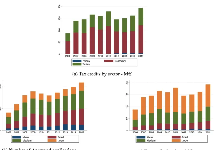
Figure 1: Total Requested and Approved tax credits - Million Euros

10_{Some firms were born after the beginning of the period. Others left the market before the end of the period} 11_{Both databases are made available by INE (Instituto Nacional de Estatística)}

Since the reintroduction of the program, both the amount of Requested and Approved tax credit have increased, as shown in Figure 1 and, with greater detail, in Table 4. The gap between the two represents requested credits that were not eligible for the program, or expenses that were not entirely accepted.

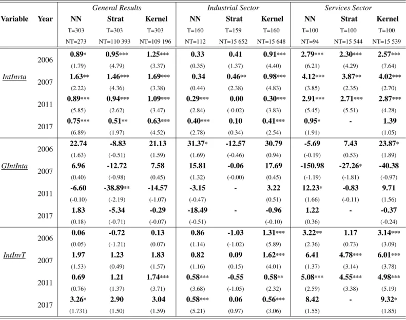
By sector, the largest share of Approved tax credit is always concentrated in the secondary sector of the economy (manufacturing industries), followed by the tertiary sector - check Figure 2a. In what regards to the firm size, although more than half of the approved applications are from small and medium firms, the largest share of approved tax credits was awarded to large firms (the weight varied between 45.4% and 56.6% across the period) - Figures 2b and 2c.

Three types of variables were used in the analysis: treatment, control, and outcome, as shown in Table 2. The treatment variable (T06) takes value 1 if the firm participated in the program in 2006 and 0 if it has never been treated. To qualify as a participant, firms must have had an approved credit greater than zero. Thus, firms with a requested amount higher than zero, and null approved tax credit are excluded from the analysis to avoid a potential bias linked to misperceptions. Firms that participate in the program for the first time in a different year are automatically excluded from the analysis since they could bias long term results.

Control variables are used as covariates in the probit model to capture the effect of observable firms’ characteristics that may influence participation. The size of the firm is controlled with both the logarithm of the number of employees (lPer) and the logarithm of the firms’ turnover12 (lT O). Note that, a priori, treated firms have, on average, 35 times more employees than non-treated ones (a proportion that goes up to 172 for intangible investment), revealing the importance of this matching process, as it minimizes pre-existing differences.

The level of investment is also believed to affect participation in the program. Hence, the logarithm of Gross Fixed Capital Formation (lGFCF) is also used as a control. One expects that firms with higher levels of investment are more prone to participate in the program.

Regional and sectoral characteristics are considered as well. Resorting to the Nomenclature of Territorial Units for Statistics (NU T S)13, the country was divided into three groups: a region that includes a metropolitan area (Lisbon and Oporto metropolitan areas), a hyper-peripheral region (as the autonomous region of the Azores and the autonomous region of Madeira), and a peripheral region (remaining regions). Thus, NU T S captures general regional effects, as firms in some regions may be more likely to invest in R&D due to surrounding dynamics.

The economic sector (Sector), on the other hand, controls for industry-specific effects. This variable reflects the fact that the probability of participating in a program is most likely larger in some sectors than in others. In the control setting, three groups14 were considered. Primary sector firms (extraction of raw materials) form the first group, while the remaining were split into two: those which are more prone to innovate (as technical, scientific, or information and communication activities) and those which are less prone to innovate (such as housing, real estate, restaurants, or social support activities).

Firms’ profitability, constructed as the ratio between net result and turnover (lNP), was included given its likely effect on R&D (less profitable firms may as well be less prone to innovate due to financial constraints). Firms’ seniority (Age) takes into account the fact that firms may behave differently across their lifetime (younger firms may focus more on R&D to stand out in the market, or older firms may have greater stability to do it, for example), being also considered.

Finally, several outcome variables were chosen to measure the outward impact of the program, allowing to test the full crowding-out hypothesis. Intangible investment as a percentage of total assets (IntInvta) is used as a proxy for the investment in R&D. For the sake of robustness, the intangible investment over Turnover (IntInvT ) was also used as an outcome variable. Given that SIFIDEwas designed as an incentive to R&D investment, participating should contribute to higher intangible investment ratios. The annual growth rate of IntInvta is also included (GIntInvta).

The effect of the program on the employability of R&D personnel is assessed in this analysis,

13_{According to the division used by all member states of the European Union (Nomenclatura das Unidades}

Territoriais para Fins Estatísticos II)

14_{Resorting to the sections of Portuguese economic sector classification (CAE Rev.3), groups were formed as follows.}

as well-designed program incentivizes firms to employ more qualified staff. In particular, wages of these specific employees are part of the eligible R&D expenditures under SIFIDE. Apparent Labour Productivity (LP), defined by the ratio between value-added and the number of employees, is also analyzed as an outcome variable. LP could be a priori larger in firms that already have the disposition to invest in R&D. The degree of openness, measured by the ratio of total export and total sales (TotExp), is considered as an outcome, as innovative firms may export more. At last, the impact on firms’ survival is measured on a variable that indicates the maximum number of years the firm has survived during the period under analysis (Survival), i.e., the difference between the lastest year of the firm and 2005.

In addition, to test the no additionality hypothesis, the variable Addit was used to measure the private effort in increasing R&D. This variable is constructed as the sum of intangible investment and R&D personnel expenses, minus the assigned tax credit, and as a percentage of total assets15. As data related to R&D personnel is only available from 2011 onwards, the additionality impact is measured five years after treatment.

In this analysis, firms with less than two employees, a Turnover lower than 2 000AC per month16, or negative intangible investment values were excluded to avoid biasedness coming from the shell and shelf firms.

Afterwards, the similarity between groups is verified for the pre-program period. Figure 3 and Table 3 present a comparison of variables’ averages before treatment, showing that participating firms already diverged from non-participating ones. However, once we restrict the comparison to the treated and control group - observations that will de facto be used to calculate average treatment effects-, these differences are significantly reduced, especially for the case of InvIntta (primary outcome for investment), where there is no statistically significant difference. It is important to note that the propensity score method does not require all firm characteristics to be similar between treated and control groups, but only their propensity scores.

15_{Given the inexistence of the variable in the database, it was estimated through the product between total personnel}

expenses and the share of workers assigned to R&D. Average tax credit built with clusters of dimension 3.

4

Result Analysis

4.1

Baseline Specification

Table 5 shows the estimation of the probit model. The balancing property is verified, and observations with propensity scores outside the common support region are omitted from the sample, ensuring a more accurate comparability17. This model allowed the selection of 303 treated firms and a control group of 109 625 firms, under the following common support region:

[0.00001, 0.95081].

4.1.1 General results

General results presented in Tables 6 and 7 are broadly consistent with the program’s expected impacts, i.e., there are significant differences in the outcomes of treated and control groups. Consequently, the full crowding-out hypothesis is rejected.

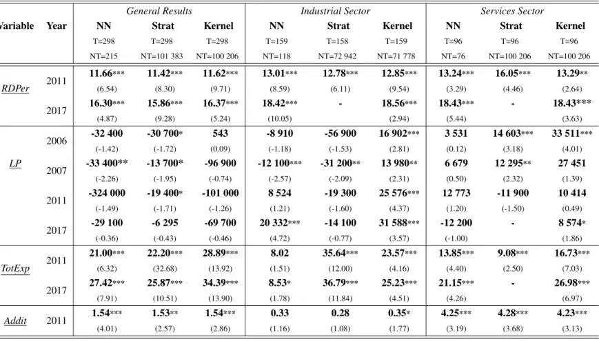
Intangible investment is higher for firms that participated in the program, as shown by the τAT T

of IntInvtta. The ratio is 0.89 pp to 1.25 pp higher in treated firms in contemporaneous terms, 1.46 pp to 1.69 pp higher one year later, and, as expected, the effects seem to diminish with time (0.51 pp to 0.75 pp, 11 years after). The impacts are unarguably more substantial for services firms when compared with the industrial ones (one-year after treatment, the ratio is higher by 0.46-0.98 pp and 3.87-4.12 pp, respectively). On the other hand, although investment seemed to grow in level terms, results for GIntInvta are not statistically significant, which may result from abnormal variations such as those in firms that had very low levels of investment (enormous variations).

IntInvT effects are non-significant for all firms, potentially due to the high volatility of the denominator (Turnover), but also exhibit positive results for the services and industrial sector. For the services sector, the impacts are increasing with time, with 6.01 pp larger for treated firms one year after treatment, which compares with 1.62 pp in the industrial sector.

Table 7 shows the program’s impacts on other outcome variables. RDPer data is only available

from 2011 onwards, making it impossible to measure contemporaneous impacts. However, participating firms have around 16 more employees assigned to R&D than the remaining ones, 11 years after treatment (firms that increase their R&D levels need to increase the number of employees to perform these specific tasks). For the apparent labour productivity (LP), results were not very consistent across matching methods nor significant in most cases. Finally, participating firms present a greater level of internationalization, although it is only possible to estimate long term results, given the lack of data. The TotExp ratio is 21.0 to 28.9 pp larger five years after the participation in the program, being the difference even greater 11 years after treatment (25.9 to 34.4 pp). That is, internationalization is positively affected, revealing potential effects in competitiveness levels, one of the main objectives of the program.

4.1.2 Survival

Regarding firms’ survival, one finds significant impacts of the program (Table 8). When considering the full period extension (11 years), treated firms survived, on average, more 0.71 to 1.1 years. Thus, SIFIDE seems to help to keep innovation in society for a longer period, assuming that R&D is effectively converted into innovation. Since the results’ magnitude may not be entirely associated with the program’s impact, one complements the analysis by exploiting survival differences among groups (distinction by size, sector, region, or profitability levels).

The effects on survival are lower in the services sector, potentially due to the pre-existing high volatility of survival in this sector. Regarding firm size, it is worth noting that small firms are those whose survival results are higher, regardless of the sector in which they are included - in general, their average survival goes up to 1.4 years longer. A sector-size cross-analysis reveals that survival in the industrial and services sector diminishes with size, from small firms onwards (same pattern as for all firms). Thereafter, regional dynamics are tested, contrasting the differences between regions that include metropolitan areas and those which do not. Estimates show that firms in Lisbon or Oporto metropolitan areas seem to survive for a more extended period (up to 1.15 years against 0.79, respectively). Finally, impacts are higher for firms with lower profits, i.e., with NP below

average in the matching period, with an average survival of 0.86 to 1.29, against 0.59 to 0.91 for high-profit firms. This break down shows that the program may be effective at reducing the firm’s solvency problems when performing R&D activities.

4.2

Robustness

One could question whether PSM results are an entire consequence of the program, given the existing gaps before the program took place in some variables’ averages among groups. When resorting to the DiD with PSM, the results, presented in Table 9, reveal that the existing differences among groups are, at least partially, linked to the program (average differences among groups raised after the program took place).

There is conformity between these results and the previous ones for IntIntta in the short term (the ratio is increased by 0.3 pp one year after treatment), but not in the long term. Differences in intangible investment in level terms are increased by 1.6 to 1.7 million euros one year after treatment, vanishing in the long term. This reinforces the rejection of the full crowding-out hypothesis, as total investment in R&D is higher for participating firms. Finally, Survival results are verified, showing that the average survival was increased by one year, as shown previously.

4.3

Additionality

Results show a rejection of the no additionality hypothesis, as illustrated in Table 7. Five-years after treatment, Addit is higher by around 1.5 pp for treated firms. Therefore, SIFIDE also seems to be able to encourage firms to increase their private effort in the innovation process, i.e., increase the amount of R&D expenditure supported by their own resources. These effects are substantially lower in the industrial sector, where the ratio is increased by at most 0.35 pp. On the other hand, services treated firms have a 4.23 to 4.28 pp higher Addit.

When analysing more contemporaneous results (Table 9), additionality can also be verified. As shown, the average increase in intangible investment, one year after treatment, is 1.59 mAC for treated firms, seven times more than the average amount of approved credit in 2006 (0.22 mAC).

5

Policy Recommendations

In sum, SIFIDE has shown to be effective in increasing investment in R&D, especially contemporaneously and one-year after treatment, and more significantly in the services sector. Besides, the program also has a side effect that can be extremely important for the conversion of R&D investment into innovation: it helps firms to survive longer. Taking these findings into account, some policy recommendations can be suggested, contributing to the improvement of the program’s efficacy.

The first recommendation is that the program should remain in place, given its effectiveness, as long as it is still believed that there is underprovision of R&D. Furthermore, it could be beneficial to introduce supplementary incentives to be awarded to specific groups, according to their response to the program. For instance, a higher base rate could be attributed to firms from the services sector or to smaller firms. This recommendation also stems from the literature that advises focusing policy incentives on the groups where they can be more effective.

As it seems, firms end up having greater relations in the foreign market after participating in the program, diversifying risk as they start depending on more than one type of market. This mechanism could encourage not only trade relations but also innovation relationships with similar peers. As such, for example, expenditures linked to cooperative R&D with foreign entities could become eligible.

Given the results on firms’ survival, the program might also include an extra incentive on this matter. Instead of indiscriminately assigning tax incentives, groups can be formed according to the results found. This extra incentive could be delayed and attributed if firms have survived and after verifying that innovation was created and persisted in that period. However, as the program intends to incentivize firms to spend more resources, it should not compromise the firms’ liquidity levels.

Summarizing, other marginal rates could be added to this mechanism, exploiting the differences in impacts found in this study. This could be relevant to increase the effectiveness of the program per se, but also to achieve other Government goals. Note that in order not to finance R&D activities fully, a maximum rate would have to be established if these additional incentives would take place.

Finally, regardless of these recommendations, accessibility to the program should keep transparent and straightforward, under the risk of losing efficient firms.

6

Conclusion

This paper had two main objectives: to evaluate the impact of the Portuguese tax incentive to R&D (SIFIDE) on R&D investment and on other related variables (such as labour productivity or the level of internationalization), and to verify whether firms’ survival is affected by this incentive (as participating firms, in theory, reduce their investment costs and potentially gain a competitive advantage attributed to innovation).

This impact evaluation was conducted resorting to Propensity Score Matching and Difference-in-Differences methodologies and using the SCIE and SIFIDE databases for the 2005-2007 period. This study contributes to the literature by analyzing the effect of tax credits on the survival of the firm, which is seldom done in the literature and, nevertheless, important in order to assess whether potential gains from innovation can be preserved. In addition, the program’s impact was analyzed over several years and across sectors and firm sizes.

The empirical results demonstrate that there is an increase in R&D investment caused by the tax incentive and that this effect can persist over time. They also show that private funding is not merely replaced by public funding, as the full crowding-out and the no additionality hypotheses are rejected. Therefore, underprovision of R&D seems to be slackened, bringing levels closer to the socially desirable. The investment impacts are higher in the services sector and one year after treatment for all types of firms. Apparent labour productivity does not appear to be impacted by SIFIDE, while the internationalization level seems to be more significant for participating firms.

Firms’ survival, especially for smaller firms and those with lower profitability and potentially lower liquidity, is positively affected by the tax incentive. Given these results, increases in the probability of maintaining innovation in the economy for a longer period are expected to happen due to the program and, consequently, positive contributions to economic growth.

7

Figures

(a) Tax credits by sector - MAC

(b) Number of Approved applications _{(c) Tax credits by size - MAC}

Figure 2: Approved applications and tax credits

(a) LogTurnover (b) LogIntangibleInvestment (c) LogGFCF

8

Tables

Table 1: SIFIDE Evolution

Designation Base Rate Incremental Rate Incremental Limit Carry-Forward

1997-2000

SIFIDE 8% 30% 250 000AC 3 years

2001-2003 20% 50% 500 000AC 6 years

2004-2005 SIFIDEwas not in force during this period

2006-2008

SIFIDEII 32.5% 750 000AC 8 years

2009-2017 1 500 000AC

Table 2: Variables Description Type Variable Description

Treatment T06 1 if participated in the program in 2006 and 0 if never participated

Control

lPer Logarithm of the total number of employees lTO Logarithm of Turnover

lGFCF Logarithm of GFCF

NTUS Nomenclature of Territorial Units for Statistics Sector Economic sector

lNP Logarithm of Net Profit ratio lAge Logarithm of Age

Outcome

IntInvta Intangible Investment (% of total assets) GIntInvta Intangible Investment (% of total assets) growth

IntInvT Intangible Investment (% of Turnover) RDPer R&D Personnel

LP Apparent Labour Productivity TotExp Total Exports (% of Turnover) Survival Survival of firms (years in operation)

Addit Intangible Investment + R&D Personnel wages - tax credit (% of total assets)

Table 3: Pre-treatment Averages Diferences (Year: 2005)

Variable Treated (1) Non-treated (2) Control (3) (2)-(1) (3)-(1) IntInv 953 406 5 537 1 333 909 -947 869*** 380 504*** IntInvta 1.7 0.4 0.9 -1.4** -0.9 lTO 16.2 12.2 15.9 -4.0** -0.2 LP 62 180 26 286 94 295 -35 894*** 32 115* GFCF 5 700 231 40 138 3 308 180 -5 660 093*** -2 392 051*** Personnel 314 9 287 -304*** -27*** NP 0.07 0.01 0.08 -0.06* 0.00 Notes: - Significance level: 1%:***, 5%:** and 10%:*.

Table 4: Tax Credits and Applications Year Total Requested Tax Credits (MAC) Total Approved Tax Credits (MAC) Percentage of Approved Tax Credits (%) Number of Approved Applications Number of Approved Applications (1sttime) 2006 109.60 86.79 79.18 404 404 2007 167.98 138.91 82.70 600 282 2008 209.60 145.54 69.43 804 289 2009 242.35 164.53 67.89 891 261 2010 219.42 159.73 72.79 839 153 2011 252.46 178.17 70.58 800 110 2012 186.52 145.37 77.94 864 179 2013 180.59 149.79 82.95 943 193 2014 179.96 160.94 89.43 992 199 2015 212.55 191.87 90.27 1093 204 Total 1 961.03 1 521.64 - - 2 274

Table 5: Propensity Score Estimation (probit model)

Number of obs 133 589 LR chi2(6) 1 719.01 Prob>chi2 0.0000 Log Likelihood -1 288.0569 Pseudo R2 0.4002

T06 Coef. Std. Err. z P>|z| [95% Conf. Interval] lPersonnel .1911752 .0291034 6.57 0.000 .1341337 .2482168 lTurnover .2131458 .0261625 8.15 0.000 .1618683 .2644234 lGFCF .131973 .0176073 7.50 0.000 .0974633 .1664826 NTUS2 1.087887 .3587714 3.03 0.002 .3847081 1.791066 NTUS3 1.221066 .3563332 3.43 0.001 .5226661 1.919467 Sector2 .8323473 .1581389 5.26 0.000 .5224008 1.142294 Sector3 .1668637 .3667561 0.45 0.649 -.551965 .8856923 lNP .2017998 .0203160 9.93 0.000 .1619812 .2416183 lAge -.1887554 .0284895 -6.63 0.000 -.2445937 -.132917 _cons -8.463676 .4810167 -17.60 0.000 -9.406452 -7.520901

Table 6: Average Treatment on the Treated Results (τAT T) - I

General Results Industrial Sector Services Sector

Variable Year NN Strat Kernel NN Strat Kernel NN Strat Kernel

T=303 T=303 T=303 T=160 T=159 T=160 T=100 T=100 T=100 NT=273 NT=110 393 NT=109 196 NT=112 NT=15 652 NT=15 648 NT=94 NT=15 544 NT=15 539 IntInvta 2006 0.89* (1.79) 0.95*** (4.79) 1.25*** (3.37) 0.33 (0.35) 0.41 (1.37) 0.91*** (4.40) 2.79*** (6.21) 2.30*** (4.29) 2.57*** (7.64) 2007 1.63** (2.22) 1.46*** (4.36) 1.69*** (3.38) 0.34 (0.44) 0.46** (2.38) 0.98*** (4.83) 4.12*** (3.85) 3.87** (2.35) 4.02*** (2.70) 2011 0.89*** (5.85) 0.94*** (2.62) 1.09*** (3.47) 0.29*** (2.84) 0.00 (-0.02) 0.30*** (3.83) 2.91*** (5.45) 2.71*** (5.51) 2.87*** (4.28) 2017 0.75*** (6.89) 0.51** (1.97) 0.63*** (4.52) 0.40*** (2.78) 0.10 (0.34) 0.41*** (2.54) 0.95* (1.91) - 1.39 (1.05) GIntInta 2006 22.74 (1.63) -8.83 (-0.51) 21.13 (1.59) 31.37* (1.69) -12.57 (-0.46) 30.79 (0.94) -5.69 (-0.19) 7.43 (0.53) 23.87* (1.89) 2007 6.96 (0.40) -12.72 (-0.98) 7.58 (0.45) 15.81 (1.32) -0.06 (-0.00) 17.69 (0.45) -150.98 (-1.19) -27.26* (-1.81) -40.38 (-0.97) 2011 -6.60 (-0.10) -38.89** (-2.19) -14.57 (-1.07) -3.15 (-0.47) - 3.22 (0.51) 12.23* (1.66) -0.83 (-0.11) 9.71 (1.56) 2017 1.83 (0.18) -5.34 (-0.71) -0.29 (-0.07) -18.49 (-0.51) - -0.96 (-0.10) 1.22 (0.36) - -0.37 (-0.24) IntInvT 2006 0.06 (0.05) -0.72 (-1.21) 0.13 (0.07) 0.86 (1.14) -1.03 (-1.02) 1.31*** (5.89) 3.22** (2.36) 1.17 (0.73) 3.14*** (3.09) 2007 1.97 (1.53) 1.23 (0.49) 1.83 (1.57) 0.82 (1.16) 0.09 (0.15) 1.62*** (4.01) 6.41 (1.37) 4.78*** (3.14) 6.01*** (3.78) 2011 0.69 (0.76) 1.21 (1.37) 1.74*** (3.71) 0.58*** (3.68) -0.55 (-1.05) 0.58** (2.32) 5.08*** (2.59) 4.55*** (3.38) 4.98*** (5.19) 2017 3.26* (1.731) 2.90 (1.50) 3.04 (1.59) 0.58*** (5.21) 0.06 (0.97) 0.56*** (3.06) 8.42 (1.55) - 9.32* (1.85) Notes: - The value in brackets refers to the t-stat (the bootstrapping process was used to estimate the variance);

- Significance level: 1%:***, 5%:** and 10%:*;

- The number of treated observations used (T) are the same for the entire column, while the non-treated value (NT) refers to the first line estimation.

Table 7: Average Treatment on the Treated Results (τAT T) - II

General Results Industrial Sector Services Sector

Variable Year NN Strat Kernel NN Strat Kernel NN Strat Kernel

T=298 T=298 T=298 T=159 T=158 T=159 T=96 T=96 T=96 NT=215 NT=101 383 NT=100 206 NT=118 NT=72 942 NT=71 778 NT=76 NT=100 206 NT=100 206 RDPer 2011 11.66*** (6.54) 11.42*** (8.30) 11.62*** (9.71) 13.01*** (8.59) 12.78*** (6.11) 12.85*** (9.54) 13.24*** (3.29) 16.05*** (4.46) 13.29** (2.64) 2017 16.30*** (4.87) 15.86*** (9.28) 16.37*** (5.24) 18.42*** (10.05) - 18.56*** (2.94) 18.43*** (5.44) - 18.43*** (3.63) LP 2006 -32 400 (-1.42) -30 700* (-1.72) 543 (0.09) -8 910 (-1.18) -56 900 (-1.53) 16 902*** (2.81) 3 531 (0.12) 14 603*** (3.18) 33 511*** (4.01) 2007 -33 400** (-2.26) -13 700* (-1.95) -96 900 (-0.74) -12 100*** (-2.57) -31 200** (-2.09) 13 980** (2.31) 6 679 (0.50) 12 295** (2.32) 27 451 (1.39) 2011 -324 000 (-1.49) -19 400* (-1.71) -101 000 (-1.26) 8 524 (1.21) -19 300 (-1.60) 25 576*** (4.37) 12 773 (1.20) -11 900 (-1.50) 10 414 (0.49) 2017 -29 100 (-0.36) -6 295 (-0.43) -69 700 (-0.46) 20 332*** (4.72) -14 100 (-0.77) 31 588*** (3.57) -12 200 (-1.00) - 8 574* (1.86) TotExp 2011 21.00*** (6.32) 22.20*** (32.68) 28.89*** (13.92) 8.02 (1.51) 35.64*** (12.00) 23.57*** (4.16) 13.85*** (4.40) 9.08*** (2.50) 16.73*** (7.03) 2017 27.42*** (7.91) 25.87*** (10.51) 34.39*** (13.90) 8.53* (1.78) 36.79*** (11.84) 25.23*** (4.51) 21.15*** (4.26) - 26.98*** (6.97) Addit 2011 1.54*** (4.01) 1.53** (2.57) 1.54*** (2.86) 0.33 (1.16) 0.28 (1.08) 0.35* (1.77) 4.25*** (3.19) 4.28*** (3.68) 4.23*** (3.13) Notes: - The value in brackets refers to the t-stat (the bootstrapping process was used to estimate the variance);

- Significance level: 1%:***, 5%:** and 10%:*;

- The number of treated observations used (T) are the same for the entire column, while the non-treated value (NT) refers to the first line estimation.

Table 8: Average Treatment on the Treated Results (τAT T) - Survival

General Results Industrial Sector Services Sector Variable Type NN Strat Kernel NN Strat Kernel NN Strat Kernel

T=303 T=298 T=298 T=160 T=155 T=160 T=100 T=91 T=100 NT=268 NT=101 383 NT=100 206 NT=108 NT=16 120 NT=15 648 NT=92 NT=13 443 NT=15 539 All 0.82*** (3.24) 0.71*** (4.33) 1.10*** (7.07) 0.99* (1.80) 0.58** (2.15) 1.01*** (3.94) 0.48 (0.88) 1.06*** (3.86) 0.78** (2.18) Micro 0.55 (0.61) -0.20 (-0.33) 0.50 (1.38) 0.88* (1.92) 0.46 (1.64) 1.13*** (8.45) 0.75 (1.39) 0.76** (2.48) 0.83*** (2.57) Survival Small 1.16** (2.10) 1.03*** (6.23) 1.38*** (5.79) 1.11*** (2.92) 0.73*** (5.07) 1.09*** (8.52) 0.78*** (2.15) 0.96*** (4.82) 1.05*** (5.74) Medium 0.97* (1.85) 0.89*** (7.08) 0.92*** (4.84) 0.88*** (2.78) 0.78*** (3.63) 1.03*** (6.14) 0.82* (1.73) 0.89*** (3.88) 0.97*** (6.36) Large 0.55 (0.80) 0.48 (0.83) 0.45 (0.93) 0.87*** (2.42) 0.69*** (3.38) 1.00*** (4.625) 0.66*** (2.92) 0.74** (2.18) 0.78*** (3.36) Metro. 1.05*** (2.39) 0.76*** (7.21) 1.15*** (5.41) Non-Metro. 0.24 (0.90) 0.42 (0.79) 0.79** (2.19) Low Profitability 1.19*** (4.73) 0.86*** (5.23) 1.29*** (2.96) High Profitability 0.66 (1.60) 0.59** (2.07) 0.91*** (3.02)

Notes: - The value in brackets refers to the t-stat (the bootstrapping process was used to estimate the variance); - Significance level: 1%:***, 5%:** and 10%:*;

- The number of treated observations used (T) are the same for the entire column, while the non-treated value (NT) refers to the first line estimation.

Table 9: Difference-in-Differences with Propensity Score Matching Independent Variable

T06*t T06 t Turnover Personnel NUTS CAE

2007 0.30** (2.20) 2.00*** (19.20) -0.02*** (-2.78) -0.00*** (-3.16) 0.00*** (6.16) 0.00*** (2.63) 0.04*** (13.58) IntIn vta 0.30** (2.18) 2.02*** (19.81) -0.02*** (-2.75) 2017 -1.03*** (-7.98) 1.98*** (19.23) -0.06*** (-7.47) -0.00 (-1.01) 0.00*** (4.16) 0.00 (1.29) 0.04*** (10.72) -1.03*** (-8.01) 2.02*** (19.93) 0.06*** (-7.18) 2007 -4.16 (-0.04) -2.39 (-0.04) -16.13 (-1.42) 0.00 (0.14) 0.01 (0.30) 0.92 (0.89) 8.14** (2.89) GIntIn vta -6.27 (-0.06) 5.11*** (0.08) -15.12*** (-1.33) Dependent V ariable 2017 2.30 (0.02) -0.89 (-0.01) -17.82 (-1.20) 0.00 (0.29) -0.00 (-0.00) 1.18 (1.08) 8.19*** (2.77) -0.93 (-0.01) 5.11*** (0.08) -16.89*** (-1.14) 2007 1 587 401*** (20.25) -1 325 112*** (-16.23) -3 577 (-0.83) 0.03*** (108.81) -817.4*** (-17.66) -367.4 (-0.34) 7 251.3** (2.46) IntIn v 1 691 208*** (21.52) 737 816** (8.80) -844.7 (-0.20) 2017 -16 154 (-0.18) -309 861.0*** (-5.05) -12 321.8** (-2.29) 0.01*** (77.95) -179.6*** (6.88) 274.4 (0.37) 3 064.9* (-1.76) 182 958** (1.98) 737 753.7*** (11.79) -4 161.9 (-0.75) 2007 -2 308.2 (-0.87) -63 794.9*** (-3.97) 473.65*** (3.24) 0.0*** (41.73) -148.7*** (-21.46) 287.58 (1.20) 2 128.5*** (3.32) LP 3 540.3 (1.33) 32 933.8** (2.08) 586.0*** (4.00) 2017 -19 587.5** (-1.99) -65 702.0*** (-4.17) 3 103.8*** (4.90) 0.00*** (54.99) -219.1*** (-35.30) 321.8 (1.39) 1 246.1** (2.05) 8 963.5 (0.90) 32 905.6** (2.10) 3 381.6*** (5.26) Survi v al 2017 0.97*** (5.70) -0.12 (-0.98) 10.21 (1107.42) 0.00*** (4.10) -0.00 (-0.07) -0.01 (-3.72) 0.08*** (23.09) 0.97*** (5.71) 0.00 (1.00) 10.21*** (1105.99) Notes: - The value in brackets refers to the t-stat;

- Significance level: 1%:***, 5%:** and 10%:*; .

9

References

Aralica, Z., & Botric, V. (2013). "Ievaluation of Research and Development Tax Incentives Scheme in Croatia". Economic research-Ekonomska istrazivanja, 26(3): 63-80.

Aristei, D., Sterlacchini, A., & Venturini, F. (2015). "The effects of public supports on business R&D: firm-level evidence across EU countries". MPRA Paper, 64611.

Arrow, K. J. (1972). "Economic welfare and the allocation of resources for invention". In Readings in industrial economics. 219-236. London: Palgrave.

Bloom, N., Griffith, R., & Van Reenen, J. (2002). "Do R&D tax credits work? Evidence from a panel of countries 1979-1997". Journal of Public Economics, 85(1): 1-31.

Busom, I. (2012). "Tax incentives or subsidies for R&D?". UNU-Merit working paper, 56.

Caliendo, M., & Kopeinig, S. (2008). "Some practical guidance for the implementation of propensity score matching". Journal of economic surveys, 22(1), 31-72.

Cefis, E., & Marsili, O. (2006). "Survivor: The role of innovation in firms’ survival". Research policy, 35(5): 626-641.

Czarnitzki, D., Hanel, P., & Rosa, J. M. (2011). "Evaluating the impact of R&D tax credits on innovation: A microeconometric study on Canadian firms". Research Policy, 40(2): 217-229.

David, P. A., Hall, B. H., & Toole, A. A. (2000). "Is public R&D a complement or substitute for private R&D? A review of the econometric evidence". Research policy, 29(4-5): 497-529.

Giovannetti, G., Ricchiuti, G., & Velucchi, M. (2011). "Size, innovation and internationalization: a survival analysis of Italian firms". Applied Economics, 43(12): 1511-1520.

Griffith, R., Sandler, D., & Van Reenen, J. (1995). "Tax incentives for R&D". Fiscal Studies, 16(2): 21-44.

hgljk,nmbvc

Hall, B. H. (1987). "The relationship between firm size and firm growth in the US manufacturing sector". Journal of Industrial Economics. 35(4): 583-606.

Hall, B. H., & Lerner, J. (2010). "The financing of R&D and innovation". In Handbook of the Economics of Innovation, Vol. 1, 609-639. Netherlands: North-Holland.

Hall, B., & Van Reenen, J. (2000). "How effective are fiscal incentives for R&D? A review of the evidence". Research policy, 29(4-5): 449-469.

Hewitt-Dundas, N., & Roper, S. (2010). "Output additionality of public support for innovation: evidence for Irish manufacturing plants". European Planning Studies, 18(1), 107-122.

Kobayashi, Y. (2014). "Effect of R&D tax credits for SMEs in Japan: a microeconometric analysis focused on liquidity constraints". Small Business Economics, 42(2): 311-327.

Mansfield, E. (1986). "Patents and innovation: an empirical study". Management science, 32(2): 173-181.

Martin, S., & Scott, J. T. (2000). "The nature of innovation market failure and the design of public support for private innovation". Research policy, 29(4-5): 437-447.

Mata, J., & Portugal, P. (1994). "Life duration of new firms". The journal of industrial economics, 227-245.

Mouqué, D. (2012). "What are counterfactual impact evaluations teaching us about enterprise and innovation support?". European Commission.

Musso, P., & Schiavo, S. (2008). "The impact of financial constraints on firm survival and growth". Journal of Evolutionary Economics, 18(2), 135-149.

hgljk,nmbvc

OECD/Eurostat. (2019). Oslo Manual 2018: Guidelines for Collecting, Reporting and Using Data on Innovation. 4th Edition. Paris/Eurostat, Luxembourg: The Measurement of Scientific, Technological and Innovation Activities, OECD Publishing.

Oliveira, F., Leitão, A., Gonçalves, A., Portugal, A., Reis, B., Pinto, D., Martins, H., Vaz, H., Santos, J., Caldeira, J., Castilho, L., Mamede, R., Nascimento, R. (2019). "Os Benefícios Fiscais em Portugal - Conceitos, Metodologia e Prática". Portuguese Government

Paff, L. A. (2005). "State-level R&D tax credits: A firm-level analysis". The BE Journal of Economic Analysis & Policy, 5(1).

Petrin, T. (2018). "A literature review on the impact and effectiveness of government support for R&D and innovation". ISIGrowth.

Radas, S., Anic, I. D., Tafro, A., & Wagner, V. (2015). "The effects of public support schemes on small and medium enterprises". Technovation, 38: 15-30.

Reinert, H., & Reinert, E. S. (2006). "Creative destruction in economics: Nietzsche, Sombart, Schumpeter". In Friedrich Nietzsche. 55-85. Boston: Springer.

Rosenbaum, P. R., & Rubin, D. B. (1983). "The central role of the propensity score in observational studies for causal effects". Biometrika, 70(1): 41-55.

Wallsten, S. J. (2000). "The effects of government-industry R&D programs on private R&D: the case of the Small Business Innovation Research program". The RAND Journal of Economics, 82-100.

Yang, C. H., Huang, C. H., & Hou, T. C. T. (2012). "Tax incentives and R&D activity: Firm-level evidence from Taiwan". Research Policy, 41(9): 1578-1588.

A

Appendix

A.1

Tax deductions vs. tax credit (illustrative example)

Tax deduction Tax credit Income before tax 1000 1000

Tax deduction x

Taxable income 1000 − x 1000 Income tax t(1000 − x) t1000

Tax credit x

Net result 1000 − t1000 + tx 1000 − t1000 + x

• Tax credit (x) is summed up to net result only if this is greater than 0;

• Tax deductions generate a lower net result than a tax credits of the same magnitude: With 0 < t < 1 and x > 0, then tx < x

⇒ 1000 − t1000 + tx < 1000 − t1000 + x ⇒ Net result_{Tax deduction} < Net result_{Tax credit}

A.2

Eligible expenses

The following points list the eligible expenditure to the program:

1) Acquisitions of property, plant and equipment, except buildings and land (in proportion to R&D activities); 2) Expenditure on staff with a minimum level of education, directly involved in research and development tasks; 3) Expenses with managers and staff in the management of R&D institutions;

4) Operating expenses, up to a maximum of 55% of expenditure (tasks accounted for as remuneration);

5) Expenses related to the contracting of R&D activities with public entities or beneficiaries of public utility status or entities whose R&D suitability is recognized by Government members;

6) Participation in the capital of R&D institutions and contributions to public or private investment funds intended to finance companies mainly devoted to R&D.

7) Patent registration and maintenance costs;

8) Expenses with the acquisition of patents that are predominantly for R&D activities; 9) Expenditure on R&D audits;

A.3

Tax credit calculation

The tax credit of firm i in time t is obtained by applying a base rate (BaseRate) to the total eligible expenses (Totit), as well as an incremental rate (IncreRate) to changes from one year to the other

(∆Totit), as in equation 6.

TaxCreditit = BaseRate ∗ Totit+ A ∗ I + (1 − A) ∗ IncreRate ∗ Totit (6)

• ∆Totit= Totit− (Totit−1+Tot₂ it−2)

• I =            0 , ∆Totit< 0

0.5 ∗ ∆Totit , ∆Totit≥ 0 V 0.5 ∗ ∆Totit< 1, 500, 000

1, 500, 000 , Otherwise • A =     

1 , Firm with 2 or more periods of exercise or large firm 0 , Otherwise