Stochastic volatility jump-diffusion models as time-changed Lévy processes

University of Lisbon

ISCTE Business School

Faculty of Sciences

University Institute of Lisbon

Department of Mathematics

Department of Finance

Stochastic Volatility Jump-diffusion Models

As Time-Changed Lévy Processes

Ricardo Matos

Dissertation

Master’s Degree in Financial Mathematics

University of Lisbon

ISCTE Business School

Faculty of Sciences

University Institute of Lisbon

Department of Mathematics

Department of Finance

Stochastic Volatility Jump-diffusion Models

As Time-Changed Lévy Processes

Ricardo Matos

Dissertation supervised by Professor João Pedro Vidal Nunes

Master’s Degree in Financial Mathematics

Acknowledgments

"Não sou nada. Nunca serei nada. Não posso querer ser nada. À parte isso,

tenho em mim todos os sonhos do mundo." Álvaro de Campos "As nossas dúvidas são traidoras,

e fazem-nos perder o que, com frequência, poderíamos ganhar,

por simples medo de tentar."

William Shakespeare "O carácter do homem é o seu destino."

Heraclitus

Gostaria de prestar os meus sinceros agradecimentos ao meu orientador, Professor Doutor João Pedro Nunes, por todo o apoio não só ao longo da tese mas também durante o mestrado. Pelo mentor e pessoa inspiradora que foi, estou sinceramente agradecido.

Gostaria também de agradecer a todas as pessoas que me apoiaram durante o meu percurso académico e em especial durante a elaboração desta tese. Agradeço a toda a minha família pelo apoio incondicional: ao meu pai, à minha mãe, à minha irmã e à Céu, por nunca deixarem de acreditar em mim. Às minhas avós, porque sei que as deixei orgulhosas.

E por fim, um agradecimento especial à Filipa por toda a compreensão, con-fiança e apoio durante esta etapa, por estar sempre ao meu lado e por fazer parte da minha vida.

Abstract

This thesis focuses on applying the time-changed Lévy processes tech-nique firstly presented by Carr and Wu (2004) in order to deduce the Bakshi et al. (1997) model with a general jump size distribution. The second goal is reach a full correlation scheme, after reaching the fundamental theo-rem, where we show how to compute the joint characteristic function of a finite number of time-changed Lévy processes under the leverage-neutral measure, we obtain an exact characteristic function for an asset price with stochastic volatility, stochastic interest rates, jumps and a full correlation scheme. As far as we know this is the first time that the exact characteristic function of an model that take into account stochastic volatility, stochastic interest rates, jumps and a full correlation scheme is achieved.

Keywords: Time-changed Lévy process. European standard call and put.

Stochastic volatility. Stochastic interest rate. Jump diffusion. Bakshi, Cao and Chen model. Full correlation. General jump size distribution.

Resumo

Esta tese foca-se na aplicação da técnica de time-changed Lévy processes, apresentada em primeiro lugar por Carr and Wu (2004), a fim de deduzir o modelo de Bakshi et al. (1997) com uma distribuição arbitrária do tamanho do salto. O segundo objectivo passa por obter um modelo com correlação total, depois de deduzir o teorema fundamental onde se obtém a função característica conjunta de um número finito de time-changed Lévy processes sob a medida de alavancagem neutra. Posteriormente, obtivémos a função característica exacta para o preço de um activo com volatilidade estocástica, taxas de juros estocásticas, saltos e correlação total. Tanto quanto sabemos, foi a primeira vez que se obteve a função característica exacta de um modelo com volatilidade estocástica, taxas de juros estocásticas, saltos e correlação total.

Palavras-chave: Time-changed Lévy process. Opção Europeia standard de

compra e venda. Volatilidade estocástica. Taxas de juro estocásticas. Difusão com saltos. Modelo de Bakshi, Cao and Chen. Correlação total. Tamanho do salto com distribuição arbitrária.

Contents

Introduction 1

1 Mathematical tools 3

1.1 Signed and complex measures . . . 3

1.2 Basic Tools . . . 5

1.2.1 Cholesky Theorem . . . 9

1.2.2 Lévy-Khinchin representation . . . 10

1.2.3 Dubins-Schwarz0s Theorem . . . 12

1.2.4 Girsanov’s Theorem . . . 13

1.2.5 Girsanov’s Theorem for Jump-Diffusion processes . . . . 14

1.2.6 Fourier Inversion Theorem . . . 16

1.2.7 Change of Numeráire . . . 17

1.2.8 Ito’s Lemma for jump-diffusion processes . . . 23

1.2.9 The Feynman-Kac Theorem . . . 24

2 Time-changed Lévy processes 25 2.1 The idea . . . 25

2.2 Affine activity rate . . . 27

2.3 Fundamental theorem . . . 29

3 Asset pricing with constant interest rates 33 3.1 Heston model . . . 35

3.2 Heston model as a time changed Lévy process . . . 37

3.3 Heston model with jumps as a time changed Lévy process . . . 44

3.3.1 Jumps with a Gaussian distribution . . . 46

4 Asset pricing with stochastic interest rates 51

4.1 Zero coupon bond . . . 53 4.2 The Bakshi, Cao and Chen (1997) model as a time changed

Lévy process . . . 55

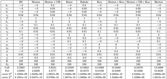
5 Numerical results 66

5.1 European call and put options . . . 67

6 A general dependency structure 71

Conclusion 85

Appendices 86

A Matlab Code function 1 87

B Matlab Code function 2 90

C Matlab Code function 3 93

D Riccati0s equation 101

Introduction

We have focused on two fundamental goals during this thesis. The first is to obtain the Bakshi et al. (1997) model with a general jump size distri-bution as a time-changed Lévy process. This technique can greatly simplify the computation of the characteristic function of the asset price through a complex-valued change of measure on one part of the time-changed Lévy process. Later on this thesis we will see that this change of measure af-fects only the instantaneous activity rate. The second goal is to preserve the stochastic volatility, stochastic interest rates and jumps presented by the Bakshi et al. (1997) model, while adding an exact full correlation scheme. Our technique can incorporate an finite number of time-changed Lévy pro-cesses and take into account their correlation. With this technique we may capture some characteristics of the asset price that otherwise we would not be able to. It could be of main importance for a large range of derivatives to have a joint characteristic function since almost all of them depend on more than one source of uncertain.

The paper that we use as starting point is Carr and Wu (2004). Never-theless, a great variety of theoretical results is obtained from Tankov and Cont (2004), Chesney et al. (2009), Pascucci (2011), Privault (2013), Shreve (2004), Bjork (1998) and Brigo and Mercurio (2006). Since one complex-valued change of measure is needed, the work of Dellacherie et al. (1992) is essential to the progress on this thesis.

This thesis is organized as follows. In the first chapter, we provide the fun-damental tools for the understanding of our work. On the second chapter we present the time-changed Lévy process technique, and the fundamental the-orem needed for writing the characteristic function of the time-changed Lévy process as a Laplace transform of business time — could be, for example, an

integrated CIR process. On the third chapter we develop the technique for pricing options within a scenario of constant interest rates using the above method. In the fourth chapter we make a generalization by allowing the in-terest rate to be itself a stochastic process, and we deduce our general model that nests all the models that we have deduced before. The fifth chapter con-tains the numerical implementation of our general method with two kinds of jump size distributions: The normal distribution and the double exponential distribution. We use a Gauss-Kronrod quadrature for the inversion of the characteristic function.

Finally, in chapter six a full correlation scheme is deduced and an exact characteristic function is computed.

Chapter 1

Mathematical tools

1.1

Signed and complex measures

In this chapter we will provide the fundamental tools that we will use in this thesis.

Definition 1.1. A Banach space is a vector space S which is equipped with a

norm ∥ . ∥ and which is complete with respect to that norm, i.e., every Cauchy sequence in S converges to a point in S. Let (xn) be a Cauchy sequence, then

there exists an element x in S such that

lim

n→∞∥ xn− x ∥= 0.

Definition 1.2. Let (X ,N ) be a measurable space and S be a Banach space.

A functionµ : N → S is a vector measure or a S-measure if:

i)µ(;) = 0;

ii) Countably additive : For any countable family (Aj)j∈J of disjoint sets in

N we have µ µ S j∈J A_j ¶ = P j∈Jµ(Aj ).

When S = R or S = C we have a signed measure and a complex

if in the "usual" definition of measure the requirement of non-negativity is removed.

Corollary 1.1. (Jordan decomposition theorem)

Every signed measure is the difference of two positive measures, at least one of which is finite.

Proof. See Cohn (1980, p. 125). ■

The representationµ = µ+_{− µ}−_{is called the Jordan decomposition ofµ.}

The measuresµ+ andµ− are called the positive part and the negative part ofµ, respectively.

Definition 1.3. Let (X ,N ) be a measurable space. A complex measure on

(X ,N ) is a function µ : N → C that satisfies:

i)µ(;) = 0;

ii) Countably additive : For any countable sequence (A_n) of disjoint sets in N we have µ µ _∞ S n=1 A_n ¶ = ∞P n=1µ(An ).

Each complex measureµ on (X,N ) can be written as µ = µ1+ ıµ2, where

µ1_andµ2 _{are finite signed measures on (X ,N ). Then, the Jordan}

decompo-sition theorem implies that each complex measureµ can be written as

µ = µ1

+− µ1−+ ıµ2+− ıµ2− where µ+1,µ1−,µ2+,µ2− are finite positive "usual"

mea-sures on (X ,N ).

Definition 1.4. Let (X ,N ) be a measurable space and f be a N -measurable

function. Then, we define the integral of f with respect to a complex mea-sureµ as follows: Z f dµ = Z f dµ1₊− Z f dµ1₋+ ı Z f dµ2₊− ı Z f dµ2₋.

Definition 1.5. A measureµ is said to be absolutely continuous with respect

toν if, for any measurable set A , ν(A) = 0 ⇒ µ(A) = 0.

Ifµ is absolutely continuous with respect to ν and ν is absolutely continuous with respect toµ then µ and ν are said to be equivalent measures which is denoted byµ ∼ ν.

Theorem 1.1. Radon-Nikodym theorem

Let (X ,N ) be a measurable space, let µ be a σ-finite1 positive measure on (X ,N ) and ν be a complex measure on (X,N ). If ν is absolutely continuous with respect to µ, then there exists a function h that satisfies ν(A) =

Z

A

h dµ for each _{A ∈ N . The function h is unique µ-almost everywhere.}

Proof. See Cohn (1980, p. 135). ■

Usually the function h is called the Radon-Nikodym derivative and is de-noted by d_dν_µ := h.

1.2

Basic Tools

Given a filtration (Ft)t∈[0,T] on a probability space (Ω,F ,P), τ is called a

Ft-stopping time if ∀t ≥ 0,{τ ≤ t} ∈ Ft. Proposition 1.1. Sampling Theorem

If (M_t)_t∈[0,T] is a martingale and ©

τ,ηª is a set of stopping times with

0 ≤ τ ≤ η ≤ T then

E[M_η/F_τ] = Mτ.

1_{A measure is calledσ-finite if a set X is a countable union of measurable sets with finite}

Proof. See Doob (1990, p. 370). ■ In particular, a martingale stopped at a stopping time is still a martin-gale.

Definition 1.6. A function f : [0_{, T] → R is cadlag if it is right-continuous}

with left limits, i.e., ∀t ∈ [0, T] the following limits exist,

f (t−) = lim

s→t,s<tf (s),

f (t+) = lim

s→t,s>tf (s),

and f (t) = f (t+).

We will denote f (t) − f (t−) by 4f (t). Of course 4f (t) will be different from 0 only when f jumps. A cadlag function may have at most a countable number of jumps or discontinuities and ∀² > 0 the number of jumps such that 4f (t) >

² should be finite.

Definition 1.7. Lévy process

A Lévy process is a stochastic process (Xt)t≥0 on (Ω,F ,P) which is cadlag

and has the following properties:

i) X0 = 0;

ii) for every increasing sequence of times t0, ..., tn, Xt0, Xt1−Xt0, ..., Xtn−Xtn−1 are independent;

iii) X_t+h− Xt has the same law of Xh; iv) ∀² > 0, lim

h→0P(|Xt+h− Xt| ≥ ²) = 0.

The last condition states that the process has at most a countable number of jumps.

Examples of Lévy processes are the Poisson process and the Wiener process (Brownian Motion). In the first case, and conditional onFs⊆ Ft for all s ≤ t,

the increments of the process follow a Poisson distribution with expected value λ(t − s), where λ > 0 is the intensity of the process. For the second case, the increments of the process follow a normal distribution with mean 0 and variance t − s.

Definition 1.8. A Poisson process (Nt)t≥0is a Lévy process that is piecewise

constant with jump size 1, where the occurrence of jumps has a Poisson dis-tribution with parameterλt, i.e.

∀n ∈ N, P(Nt= n) = e−λt (λt) n n! ,

and the characteristic function is given by:

E£ eıuNt¤ = eλt(eıu−1) _{, u ∈ R.}

Definition 1.9. A compound Poisson process is a stochastic process (Z_t)_t≥0 with intensityλ > 0 and jump size distribution f such that

Zt= Nt P

i=1

Yi,

where Yi are i.i.d. random variables that represent the jump size and

fol-low a distribution f while Nt is a Poisson process with intensity λ that is

independent from Yi.

Definition 1.10. Lévy measure

If (Xt)t≥0is a Lévy process, the Lévy measureν of X is defined by:

ν(A) = E[#{t ∈ [0,1] : 4Xt6= 0, 4Xt∈ A}], A is Borelian.

ν(A) is the expected number, per unit time, of jumps whose size belongs

to A. Furthermore if (Xt)t≥0 is a compound Poisson process with intensityλ

Definition 1.11. Quadratic variation

If (Xt)t≥0 is a Lévy process,2its quadratic variation is the adapted cadlag

process defined by:

[X, X ]t= |Xt|2− 2 t

Z

0

X_u−dXu.

Definition 1.12. Quadratic covariation

Given two Lévy processes (Xt)t≥0and (Yt)t≥0, the Lévy process defined by

[X, Y ]t= XtYt− X0Y0− t Z 0 X_u−dYu− t Z 0 Y_u−dXu,

is called the quadratic covariation of X and Y .

The quadratic covariation has the following important properties:

i) If X, Y are Lévy processes andϕ1,ϕ2are integrable predictable

processes, then ·Z ϕ1dX, Z ϕ2dY ¸ t = t Z 0 ϕ1ϕ2d[X, Y];

ii) The quadratic covariation is not affected by the drift term in X or Y, it is

only sensitive to the martingale term.

Example 1.1. If we consider the Brownian motion defined by Zt= σWt, by

Definition 1.11 its quadratic variation is:

[Z, Z]t= σ2Wt2− 2σ2 t

Z

0

W_udWu.

2_{A more general definition can be obtained if we consider a semi-martingale instead of a}

Lévy process, but for our purposes we will just consider Lévy processes. Particular cases of semi-martingales are the Wiener process, Poisson process and all Lévy processes.

Applying Ito’s Lemma to _{f (x) = σ}2x2, we have: σ2_W2 t = 2σ2 t Z 0 WudWu+ σ2t, so we conclude that [Z, Z]t= σ2t.

1.2.1

Cholesky Theorem

Theorem 1.2. Cholesky Theorem

If A is a real, symmetric and a positive definite matrix, then it has a unique factorization, _{A = L.L}T, where L is a lower triangular matrix with positive diagonal.3

Proof. See Kincaid and Cheney (2001, p. 157). ■

Remark 1.1. Consider two correlated Brownian Motions, fW₁andWf₂, and a third one uncorrelated with the other twoWf₃, with a correlation matrix

C =   1 _{ρ 0} ρ 1 0 0 0 1  , ρ ∈ [−1,1],

C is real and symmetric. It is also definite positive because its eigenvalues are positive in the case ofρ ∈ (−1,1); even if ρ = −1 or ρ = 1 it is easy to show that the Cholesky factorization is still verified.

Its Cholesky factorization is _{C = L.L}T, where

L =   1 0 0 ρ p1 − ρ2 ₀ 0 0 1  , ρ ∈ [−1,1].

3_{The matrix L can be found via a Cholesky factorization algorithm — see Kincaid and}

Moreover, if we consider three independent Brownian motions, W1, W2

andW₃, it can be shown — see Korn et al. (2010, p. 113) — that:

   f W₁ f W₂ f W3    =L.   W1 W₂ W₃  .

1.2.2

Lévy-Khinchin representation

Theorem 1.3. Lévy-Khinchin representation

If (Xt)t≥0is a Lévy process with characteristic triplet (µ,σ,ν), then φXt(θ) ≡ E £e

ıθXt¤ = e−tΨx(θ)_, θ ∈ R, and the characteristic exponentΨ_x(θ) is given by:4

Ψx(θ) =1₂σθ2− ıµθ −

Z

R

³

eıθx_{− 1 − ıθx}Π_|x|≤1´ν(dx).

Proof. See Tankov and Cont (2004, p. 83). ■

Remark 1.2. The Lévy process is specified by the Lévy triplet (µ,σ,ν).

Intu-itively, _{µ can be seen has the drift of the continuous part of the Lévy process,}

σ is the variance of the Brownian motion and ν is the Lévy measure.

In Theorem 1.3 we truncate the jumps larger than 1, but there are other for-mulations of the theorem, where we use a function z(x) that obeys to certain regularity conditions instead ofΠ_|x|≤1;z(x) is called the truncation function. Different choices of z(x) do not affectσ and ν but µ is affected by z(x). If the Lévy measure satisfies the condition

Z

|x|≥1

|x|ν(dx) < ∞, we can use a simpler form for the expression of the characteristic exponentΨ_x(_θ):

4_Π

Ψx(θ) =1₂σθ2− ıµθ −

Z

R

(eıθx− 1 − ıθx)ν(dx).

Proposition 1.2. A Lévy process has piecewise constant trajectories iff its

Lévy triplet has the form (µ,0,ν) with µ = Z |x|<1 xν(dx) that satisfies Z R ν(dx) <

∞. In this case, its characteristic exponent has the form: Ψx(θ) =

Z

R

(1 − eıθx)ν(dx). (1.2.1)

Proof.

By Theorem 1.3 we know that the characteristic exponent has the form: Ψx(θ) = −ıµθ − Z R (eıθx− 1 − ıθxΠ|x|≤1)ν(dx), that is: Ψx(θ) = −ıµθ + ıθ Z |x|<1 xν(dx) − Z R (eıθx− 1)ν(dx). (1.2.2) Since Z |x|<1 xν(dx) = µ,

equation (1.2.1), follows immediately from equation (1.2.2). ■

Example 1.2. Consider the compound Poisson process (Zt)t≥0 with intensity λ. Since this process has piecewise constant trajectories, the Lévy triplet is

(b, 0,ν) with b = Z

|x|<1

xν(dx), and assume that the jump size distribution is Gaussian with meanµ and variance σ2, that is:

f (x) =p 1 2πσ2e

Sinceν(dx) = λf (dx), we have: ν(dx) = λ_p 1 2πσ2e −(x−µ) 2 2σ2 dx.

Then the characteristic exponentψx(θ) of such process is:

Ψx(θ) = Z R (1 − eıθx)λ_p 1 2πσ2e −(x−µ) 2 2σ2 dx, that is: Ψx(θ) = λ  − Z R eıθx_p 1 2πσ2e −(x−µ)_2σ22 dx + Z R 1 p 2πσ2e −(x−µ)_2σ22 _dx  . (1.2.3)

The second term on the right-hand of the equation (1.2.3) is one by defini-tion of a probability density funcdefini-tion and the first term is the characteristic function of a normal random variable. Therefore:

Ψx(θ) = λ h 1 − eıθµ−12σ 2_θ2i . (1.2.4)

1.2.3

Dubins-Schwarz

s Theorem

Theorem 1.4. Dubins-Schwarz0s Theorem

A martingaleM such that [M, M]_∞= ∞ is a time changed Brownian mo-tion, i.e., there exists a Brownian motionW such that:

M_{t= W[M,M]t}.

In particular, ifξ satisfies the usual conditions for the Itô’s integral to be well defined, then X =

Z

ξ dW is a martingale because is the Itô’s integral

and its quadratic variation is [X, X ]t= t Z 0 ξ2 sds.5 Therefore, t Z 0 ξ dW = Wt R 0 ξ2 sds , for a Brownian motion W.

1.2.4

Girsanov’s Theorem

Theorem 1.5. Girsanov’s Theorem

LetP and Q be equivalent measures and (Ω,F ,P) be a measurable space. Consider the following Itô’s process :

dXt= a(t, X ) dt + b(t, X ) dWt, (1.2.5)

and consider the process (Lt)_t∈[0,T] that satisfies the Novikov0s condition6and

is defined as L_{t= e} t R 0θ sdWMs−12 t R 0θ 2 sds with EP[Lt] = 1. (1.2.6)

Consider also that the Brownian motionsW and WM are correlated with correlation d < W,WM>t= ρ dt. Then, we have the following results:

5_{It is simply necessary to apply Itô’s lemma to f (x) = x}2_. 6_EP  e 1 2 T R 0 θ2 sds 

 < ∞. This condition is sufficient to ensure that (Lt)_t∈[0,T] is a

i) LT defines a Radon-Nikodym derivative7

dQ

dP = LT, (1.2.7)

sinceL_Tis a martingale, we have: dQ dP ¯ ¯ ¯ ¯Ft= L_T L_t; (1.2.8)

ii) WQ is a new Brownian motion in (Ω,F ,Q) and is defined by:

dWQ_t = dWt− θtd < W,WM>t= dWt− ρθtdt; (1.2.9) iii) The process Xt takes the following form underQ:

dXt= a(t, X ) dt + b(t, X ) dWt= a(t, X ) dt + b(t, X )(dWQ_t + ρθtdt) (1.2.10)

= (a(t, X ) + b(t, X )ρθt) dt + b(t, X ) dWQ_t. (1.2.11)

Proof. See Zhu (2010, p. 13). ■

1.2.5

Girsanov’s Theorem for Jump-Diffusion processes

Theorem 1.6. Girsanov’s Theorem for Jump-Diffusion processes

Let Q and Q be equivalent measures, and (e Ω,F ,Q) a measurable space. Let Z_t=

Nt P

i=1

Y_i be a compound Poisson process with intensityλ and a jump size distribution f .

Consider the following Radon-Nikodym derivative deQ dQ= e T R 0 θsdWMs−12 T R 0 θ2 sds e(λ−λ)Te NT Y i=1 e λf (Ye _i) λf (Yi) . (1.2.12)

7_{Usually in the literature, L}

t is strictly positive andQ is the "usual" measure but Lt

can be real or complex valued — see Beghdadi-Sakrani (2002, p. 375) and Dellacherie et al. (1992, p. 350) — andQ a complex measure.

Consider also that the Brownian motionsWQandWMare correlated with correlation d < WQ, WM>t= ρ dt. Then under the new measure eQ, the process

dWQe t = dW Q t − θtd < WQ, W M >t= dWQ_t − ρθtdt, (1.2.13) is a Brownian motion in (Ω,F ,Q).e

Furthermore, under the new measure Q, the compound Poisson processe has the following parameters:

e λ = λE³eY´, (1.2.14) and e f (Yi) = eYi_{f (Y} i) E¡ eY¢ . (1.2.15)

AndY follows the same distribution, f , as the i.i.d. random variables Y_i.

Proof. See Shreve (2004, p. 502). ■

Remark 1.3. Using equations (1.2.14) and (1.2.15), equation (1.2.12) can be

rewritten as: deQ dQ= e T R 0θ sdWMs−12 T R 0θ 2 sds e(λ−λE(e Y₎ )T+NTP i=1 Yi . (1.2.16)

Since the right-hand side of equation (1.2.16) is a martingale, we have: deQ dQ ¯ ¯ ¯ ¯Ft= e T R tθs dWMs−12 T R tθ 2 sds e(λ−λE(e Y ))τ+NTP i=1 Yi− Nt P i=1 Yi , τ := T − t.

1.2.6

Fourier Inversion Theorem

Theorem 1.7. Fourier Inversion Theorem

Let f_X(x) be the probability density function of the random variable X andF_{X(x) = P(X ≤ x) be the distribution function. We define}

φX(ξ) ≡ E £eıξX¤ =

Z

R

eıξxf_X(x) dx

as the characteristic function of X . Then, f_{X(x) =} 1 2π Z R e−ıξxφ_X(ξ) dξ, (1.2.17) and F_{X(x) =} 1 2+ 1 2π +∞ Z 0 eıξxφX(−ξ) − e−ıξxφX(ξ) ıξ dξ. (1.2.18)

Proof. See de Figueiredo (2012, p. 203) for equation (1.2.17) and Kendall

and Stuart (1977, p. 98) or Gil-Pelaez (1951) for equation (1.2.18). ■

Remark 1.4. Equation (1.2.18) can be restated as:

F_{X(x) =}1 2+ 1 2π +∞ Z 0 eıξxφX(−ξ) ıξ + e−ıξxφX(ξ) −ıξ dξ.

Since eıξx is the complex conjugate of e−ıξx and φX(−ξ) is the complex

conjugate of φ_X(ξ), then eıξxφX(−ξ) is the complex conjugate of e−ıξxφX(ξ),

consequently eıξxφX(−ξ)

ıξ is the complex conjugate of

e−ıξxφX(ξ) −ıξ . Because z + z = 2R e(z), ∀z ∈ C, we have: F_{X(x) =} 1 2− 1 π +∞ Z 0 R e ·_e−ıξxφ X(ξ) ı_ξ ¸ dξ. (1.2.19)

1.2.7

Change of Numeráire

A numeráire is a strictly positive stochastic process (Nt)t∈R+, that is adapted toFt. The relative price of an asset St in terms of the numeráire Ntis given

by

ˆ S_t:= St

N_t, t ∈ R

+_.

Consider that (rt)t∈R+ denotes anF_t-adapted interest rate process. The discounted price, ˆS_t, is the price St, expressed in terms of the numeráire

N_{t= e} t R 0 rsds .

The risk neutral measure,Q, is a measure under which the discounted price process ˆ S_t= St N_t = e − t R 0 rsds S_t, t ∈ R+, is a martingale.

Assumption 1.1. Consider a generic numeráire (N_t)_t∈R+, the discounted nu-meráire ˆ Nt= e − t R 0 rsds Nt,

is a martingale under the risk neutral measureQ.

Definition 1.13. Taking the process (N_t)_t∈R+ as the numeráire, the forward measureQT is defined by the following Radon-Nikodym derivative:

dQT dQ = e − T R 0 rsdsN_T N₀.

Remark 1.5. Note that Definition 1.13 is equivalent to stating EQT(ξ) = EQ  e− T R 0 rsdsN_T N₀ξ  ,

for every integrableF_T-measurable random variableξ.

Theorem 1.8. We have dQT dQ ¯ ¯ ¯ ¯Ft= e − T R t rsdsN_T N_t, 0 ≤ t ≤ T. Proof.

We want to proof that

EQT(ξ|Ft) = EQ  e− T R t rsdsN_T N_tξ ¯ ¯ ¯ ¯Ft  .

Consider thatξ is integrable and FT-measurable. Then, for every

inte-grable andFt-measurable random variableÅ, we have:

EQT(Åξ|Ft) = ÅEQ T

(ξ|Ft) .

Using Remark 1.5, we know that: EQThÅEQT(ξ|Ft) i = EQT h EQT(Åξ|Ft) i = EQT[Åξ] = EQ  e− T R 0 rsdsN_T N₀Åξ   = EQ  e− t R 0 rsdsN_t N₀ÅE Q  e− T R t rsdsN_T N_tξ ¯ ¯ ¯ ¯Ft     = EQT  ÅEQ  e− T R t rsdsN_T N_tξ ¯ ¯ ¯ ¯Ft    .

Finally, it follows that EQT(ξ|Ft) = EQ  e− T R t rsdsN_T Ntξ ¯ ¯ ¯ ¯Ft  . ■

Proposition 1.3. The price at time t, of an option with an F_T-measurable payoffξ is: O_{t= E}Q  e− T R t rsds ξ ¯ ¯ ¯ ¯Ft  = N_tEQ Tµ ξ N_T ¯ ¯ ¯ ¯Ft ¶ . Proof.

From Theorem 1.8, we have:

O_{t= E}Q  e− T R t rsds ξ ¯ ¯ ¯ ¯Ft   = EQ  e− T R t rsdsN_T N_t Nt N_Tξ ¯ ¯ ¯ ¯Ft   = EQT µ_N t N_Tξ ¯ ¯ ¯ ¯Ft ¶ = NtEQ Tµ ξ NT ¯ ¯ ¯ ¯Ft ¶ , 0 ≤ t ≤ T. ■ Theorem 1.9. Given dQT dQ = e − T R 0 rsdsN_T N₀, and a Brownian motionW_t underQ, we have:

dWQ_tT = dWQ_t − 1

N_t dNtdW

Q t ,

Proof. We defineΦt as: Φt= EQ µdQT dQ ¯ ¯ ¯ ¯Ft ¶ = EQ  e− T R 0 rsdsN_T N₀ ¯ ¯ ¯ ¯Ft  , t ∈ [0, T]. (1.2.20)

The right-hand side of equation (1.2.20) is a martingale under Assump-tion 1.1. Then, using a more general version Girsanov’s Theorem — see Privault (2013, p. 276) and Protter (2004, p. 132) — we have:

dWQ_tT= dWQ_t − 1 Φt

dΦtdWQ_t, (1.2.21)

where W_tQT is aQT-Brownian motion.

Using Assumption 1.1, equation (1.2.20) becomes:

Φt= e − t R 0 rsdsN_t N₀, 0 ≤ t ≤ T. Applying Ito’s Lemma to

f (t, x) = x N0 e− t R 0 rsds , and since ∂f ∂x = e− t R 0 rsds N₀ , ∂f ∂t = − x N₀rte − t R 0 rsds , we have: d f (t, Nt) = − Nt N₀rte − t R 0 rsds dt +e − t R 0 rsds N₀ dNt,

which is the same as:

dΦt= −rtΦtdt +Φ t

N_t dNt. (1.2.22)

Taking equation (1.2.21), and using equation (1.2.22), we have: dWQ_tT= dWQ_t − 1 N_t dNtdW Q t + rtdt dW Q t, since dt dWQ_t = 0 we have: dWQ_tT = dWQ_t − 1 Nt dNtdWQ_t . ■

Remark 1.6. Consider the forward numeráire, N_{t= P(t, T), that is the price}

of a bond at time t, with maturity T:

P(t, T) = EQ  e− T R t rsds¯_¯ ¯ ¯Ft  , P(T, T) = 1. Then, dQT dQ ¯ ¯ ¯ ¯Ft= e − T R t rsdsP(T, T) P(t, T) = e − T R t rsds EQ  e T R t rsds¯¯ ¯ ¯Ft  .

The discounted bond price process  e− t R 0 rsds P(t, T)   t∈[0,T] , is aQ-martingale, because: EQ  e− t R 0 rsds P(t, T) ¯ ¯ ¯ ¯Fu  = EQ  e− t R 0 rsds EQ  e− T R t rsds¯_¯ ¯ ¯Ft   ¯ ¯ ¯ ¯Fu   = EQ  EQ  e− T R 0 rsds¯_¯ ¯ ¯Ft   ¯ ¯ ¯ ¯Fu   = EQ  e− T R 0 rsds¯_¯ ¯ ¯Fu  

= e− u R 0 rsds EQ  e− T R u rsds¯_¯ ¯ ¯Fu   = e− u R 0 rsds P(u, T), u ≤ t.

From Proposition 1.3, we have:

Ot= EQ  e− T R t rsds ξ ¯ ¯ ¯ ¯Ft  = P(t, T)EQ Tµ ξ ¯ ¯ ¯ ¯Ft ¶ , 0 ≤ t ≤ T.

Moreover, from Theorem 1.9, we have: dWQ_tT= dWQ_t − 1

P(t, T)dP(t, T) dW

Q

t. (1.2.23)

Remark 1.7. Consider the numeráire, N_{t= St}eqt, where q is the dividend yield, then: dQT dQ ¯ ¯ ¯ ¯Ft= e − T R t rsdsS_TeqT S_teqt = ST S_t e − T R t rsds eqτ, τ := T − t. (1.2.24)

Here the discounted asset price process  e− t R 0 rsds Steqt   t∈[0,T] is aQ-martingale, by the very definition of the processS_t, under the measureQ, with a dividend yield q.

From Proposition 1.3, and using ξ = S_Tξ0, where ξ0 is F_T-measurable, we have: O_{t= E}Q  e− T R t rsds S_Tξ0 ¯ ¯ ¯ ¯Ft   = SteqtEQ Tµ S_Tξ0 S_TeqT ¯ ¯ ¯ ¯Ft ¶ = Ste−qτEQ Tµ ξ0 ¯ ¯ ¯ ¯Ft ¶ . Furthermore, from Theorem 1.9, we have:

dWQ_tT= dWQ_t − 1 Steqt

dSteqtdWQ_t.

1.2.8

Ito’s Lemma for jump-diffusion processes

Lemma 1.1. Ito’s Lemma for jump-diffusion processes

Let X be a diffusion process with jumps defined by:

X_{t= X0+} t Z 0 µ(s, Xs) ds + t Z 0 σ(s, Xs) dWs+ Nt X i=1 ∆X_i, whereµ(t, X_t) andσ(t, Xt) are continuous adapted processes with

E   T Z 0 σ2_{(s, X} s) ds  < ∞.

Then, for anyC1,2 function, _{f : [0, T] × R → R, the process Yt= f (t, Xt}) can be represented as: f (t, Xt) = f (0, X0) + t Z 0 ·∂f ∂s(s, Xs) + µ(s, Xs) ∂f ∂x(s, Xs) ¸ ds +1 2 t Z 0 σ2 (s, Xs)∂ 2_f ∂x2(s, Xs) ds + t Z 0 σ(s, Xs)∂f ∂x(s, Xs) dWs + X {i≥1,Ti≤t} £ f (XT_i−+∆Xi) − f (XT_i−)¤ .

In differential notation we have:

dYt=∂f ∂t(t, Xt) dt + µ(t, Xt) ∂f ∂x(t, Xt) dt + 1 2σ 2 (t, Xt)∂ 2_f ∂x2(t, Xt) dt + σ(t, Xt)∂f ∂x(t, Xt) dWt+ [ f (Xt−+∆Xt) − f (Xt−)] .

1.2.9

The Feynman-Kac Theorem

Theorem 1.10. The Feynman-Kac Theorem

Assume that x_t is an Ito’s process that follows the stochastic process

dxt= µ(xt, t) dt + σ(xt, t) dWt.

Let V (xt, t) ∈ C2,1[R × [0,∞) → R], and suppose that V (xt, t) is the solution of

the following PDE

∂V ∂t + µ(xt, t) ∂V ∂x + 1 2σ 2 (xt, t)∂ 2_V ∂x2 − r(xt, t)V (xt, t) = 0,

with boundary conditionV (XT, T), and r(xt, t) ∈ C (R,[0,∞)). Then V (xt, t) is

given by V (xt, t) = E  e− T R t r(xu,u) du V (XT, T) ¯ ¯ ¯ ¯Ft  .

Note that the Feynman-Kac theorem can be used in both directions.

Proof. See Zhu (2010, p. 8). ■

For a Feynman-Kac Theorem for jump-diffusion processes see Chesney et al. (2009, p. 557).

Chapter 2

Time-changed Lévy processes

2.1

The idea

Since the pioneering work of Black and Scholes (1973), many studies of times series of asset returns and derivatives prices have been made, and the conclusion usually obtained is that the classic Black-Scholes option pricing model fails to explain at least three facts:

i) Asset prices have discontinuities, or commonly said, asset prices jump.

This feature was firstly discussed by Merton (1976).

ii) The volatility of asset returns varies stochastically over time. Heston

(1993) used a mean reverting square root process to model volatility.

iii) Asset returns and their volatility are correlated. This was first

discussed by Black (1976) as the "leverage effect".

Time-changed Lévy processes can capture all these three empirical find-ings. To capture the stochastic volatility, a stochastic time change to the Lévy process is made. This stochastic time change has to obey to certain conditions: It has to be positive and non-decreasing since it is describing a clock on which the Lévy process is running. The difference to the "origi-nal clock" is that randomness in business activity generates randomness in volatility, so in periods of high business activity the volatility tends to be also higher. In order to capture the correlation in asset returns and their volatility, the Lévy process is allowed to be correlated with the stochastic

time change. The jumps in asset prices are easily introduced in these mod-els and it is easy to determine the characteristic function of such processes because the time-changed Lévy process and their jumps are uncorrelated. With this feature, these models become much more realistic because heavy tails and sudden movements in asset prices are generic properties of these models. The markets in such scenario are incomplete, which can be seen as an advantage if we want a more realistic model, because some risks can not be hedged and perfect hedge does not exist.

In order to describe these models, we will follow the approach of Carr and Wu (2004).

Consider a Lévy process (Xt)t≥0 and letF be the σ-algebra generated by

the past values of the process (Xt)t≥0, completed by the null setsN ,1i.e.

F = σ(Xt, t ≥ 0)WN ,

and let (Ω,F ,P) be a probability space with a filtration (Ft)t≥0.

Let Ttbe an increasing cadlag process such that for each fixed t, {Tt≤ t} ∈

Ft, this is, Tt is a stopping time with respect toF . Consider that Tt → t→∞∞

and is finiteP − a.s.. We define

T_t:=

t

Z

0

v(s) ds (2.1.1)

as the business time where v(t) is the instantaneous activity rate, which is a positive cadlag process. The family of stopping times (Tt)t≥0 defines a

ran-dom time change.

If we evaluate the Lévy process (Xt)t≥0 at the random time (Tt)t≥0, we

obtain a time-changed Lévy process (Yt)t≥0 denoted by

Y_{t≡ XTt}, (2.1.2)

and we define its characteristic function as

1_{Notice that null sets are stuffed into F}

0, meaning that if a certain evolution of X is

φYt(ξ) ≡ E h

eıξYti_{= E}h_eıξXTti_{. (2.1.3)} When we consider a parameterξ that belongs to the complex plane, φYt(ξ) is called the generalized Fourier transform — see Titchmarsh (1948, p. 4– 44).

This kind of process has already been studied in the literature — see Tankov and Cont (2004, p. 108–113) and Pascucci (2011, p. 471). The tech-nique used is called subordination and like the techtech-nique above it simply makes a random time change in a Lévy process. In this context, the busi-ness time is called the subordinator and has the same characteristics as Tt.

Usually, the random time change is made on a Brownian motion and the subordinators are processes like the Gamma process, Inverse Gaussian pro-cess, Variance Gamma or Normal inverse Gaussian. The subordination tech-nique assumes that the subordinator and the Lévy process are independent processes. The subordinator can be any Lévy process; it is a pure jump pro-cess of possibly infinite activity plus a deterministic linear drift. Therefore the time change can have jumps and not be absolutely continuous. Under our approach, the time change will always be absolutely continuous; v(s) can exhibit jumps, but Ttis always continuous. We assume that the time change

and the Lévy process are correlated. However, if the subordinator and the Lévy process are independent, the time changed process still remains a Lévy process — see Pascucci (2011, p. 472).

In this thesis, we will focus on an integrated CIR — see Tankov and Cont (2004, p. 476) — process for the business time; some details about this pro-cess are given later.

2.2

Affine activity rate

In this section we will follow Carr and Wu (2004).

Let Xt be a Markov process that starts at X0 and satisfies the following

stochastic differential equation (SDE):

dXt= µ(Xt) dt + σ(Xt) dWt+ q dJ(γ(Xt)). (2.2.1)

γ(Xt) and jump size distribution q. Some technical conditions are required

for µ(Xt) andσ(Xt), in order to the SDE (2.2.1) to have a strong solution —

see Proposition 1 of Duffie et al. (2000, p. 1351).

Definition 2.1. The Laplace transform of the stopping time Tt is:

LTt(λ) ≡ E h

e−λTti_{. (2.2.2)}

Proposition 2.1. If the instantaneous activity rate v(s), the driftµ(X_t), the diffusion variance σ(X_t)2 and the intensity γ(X_t) are all affine in Xt and if µ(Xt) and σ(Xt) satisfy some technical conditions stated in Proposition 1 of

Duffie et al. (2000), then the Laplace transform (2.2.3) is exponential affine in X₀. That is, if 1. _{v(t) = bv}X_{t+ cv}, 2. µ(Xt) = a − kXt, 3. σ(Xt)2= α + βXt, 4. γ(X_{t) = aγ}+ bγXt, then LTt(λ) = e−b(t)X 0−c(t)_{, (2.2.3)} where b0_{(t) = λbv− kb(t) −}βb(t) 2 2 − bγ ¡ φq(ib(t)) − 1¢ , (2.2.4) and c0_{(t) = λcv+ ab(t) −}αb(t) 2 2 − aγ ¡ φq(ib(t)) − 1¢ , (2.2.5) with b(0) = c(0) = 0.

Proof. The proof follows from applying the generalized Itô’s lemma to

(2.2.3) and using SDE (2.2.1). See Duffie et al. (2000, p. 1351).

2.3

Fundamental theorem

Theorem 2.1. Fundamental theorem of time-changed Lévy processes

The generalized Fourier transform of the time-changed Lévy processYT≡

X_TT is given by:

φYT(ξ) ≡ E Ph

eıξYTi_{= E}Ph_eıξX_TTi_{= E}Q(ξ)h_e−TTΨx(ξ)i_{≡ L}Q(ξ)

TT (Ψx(ξ)). (2.3.1) Q(ξ) is a complex valued measure that is absolutely continuous with re-spect toP, and its Radon-Nikodym derivative is given by:2

dQ(ξ)

dP ≡ MT(ξ) = e

ıξYT+TTΨx(ξ)_, ξ ∈ C

ξ, (2.3.2)

whereC_ξ is the subset ofC where φ_YT(ξ) is well defined. And sinceM_t(ξ) is a complex valued martingale, we have:

dQ(ξ) dP ¯ ¯ ¯ ¯ Ft ≡ MT(ξ) M_t(ξ) = e ıξ(YT−Yt)+(TT−Tt)Ψx(ξ)_, ξ ∈ C ξ. Notice thatL_TQ(ξ)

T is not the usual Laplace transform because of the de-pendence of the measureQ(ξ) on ξ. We recall that given a process (Xt)t∈[0,T]

its Laplace transform is given by: LXT(ξ) ≡ E

h

e−ξXTi_{= φ}

XT(ıξ), ξ ∈ Cξ, (2.3.3) where C_ξ is the subset ofC where LXT(ξ) is well defined — see Titchmarsh (1948, p. 6).

Proof.

i) Consider the σ-algebra generated by the past values of the processes

(Yt)t∈[0,T] and (Tt)t∈[0,T], completed by the null sets, i.e.

2_{The measure Q(ξ) is equivalent to P but is not a probability measure, i.e., Q}(ξ)_{(Ω) 6= 1.}

G = σ(Yt, Tt, t ∈ [0, T])WN ,

and let (Ω,G ,P) be a probability space with a filtration (Gt)t∈[0,T].

First we need to proof that Mt(ξ) is a complex valuedP-martingale with

re-spect to (Gt)t∈[0,T]. Let us define Mt1(ξ) ≡ eıξXt+tΨx(ξ).

a) M1_t(_{ξ) is adapted to the filtration generated by the process (X}t)t∈[0,T]

completed by the null sets, (Ft)t∈[0,T]. b) EP£¯ ¯M1_t(ξ)¯¯¤ ≤ ¯¯eıξXt¯ ¯ ¯ ¯etΨx(ξ)¯ ¯= ¯ ¯eı(a+ıb)Xt¯ ¯ ¯ ¯etΨx(ξ)¯ ¯= ¯ ¯eıaXt−bXt ¯ ¯ ¯ ¯etΨx(ξ)¯ ¯≤

≤¯¯eıaXt¯_¯¯_¯e−bXt¯_¯¯_¯etΨx(ξ)¯_¯=¯_¯e−bXt¯_¯¯¯_etΨx(ξ)¯_{¯< ∞, a, b ∈ R,}

sinceΨx(ξ) and Xtare both finite by definition.3 c) For 0 ≤ s < t we have: EP · M1_t(ξ) M1 s(ξ) ¯ ¯ ¯ ¯ X_s ¸ = EP · eıξ(Xt−Xs)+(t−s)Ψx(ξ) ¯ ¯ ¯ ¯ X_s ¸ = e(t−s)Ψx(ξ)_EP · eıξ(Xt−s) ¯ ¯ ¯ ¯ X_s ¸ = e(t−s)Ψx(ξ)_e−(t−s)Ψx(ξ)_{= 1.}

Therefore, M1_t(ξ) is a complex valuedP-martingale with respect to (Ft)t∈[0,T].

By abuse of language we denote that filtration by Xs. For each fixed t ∈

[0, T] , Tt is a stopping time that is finite P-a.s.. Therefore, by Proposition

1.1, Mt(ξ) = M1_Tt(ξ) is a complex valued P-martingale with respect to the

(Gt)t∈[0,T]. ii) φYT(ξ) ≡ EP£ e ıξYT¤ = EP£ eıξYT+TTΨx(ξ)−TTΨx(ξ)¤ = EP£M T(ξ)e−TTΨx(ξ) ¤ = EQ(ξ)£ e−TTΨx(ξ)¤ = LQ(ξ) TT (Ψx(ξ)). ■

Remark 2.1. If the random time TT is independent of XT, no measure

change is required. By the tower rule, we have:

φYT(ξ) = EP h eıξXTTi_{= E}P · EP · eıξXTT Á T_{T= u} ¸¸ .

The outside expectation is taken on all possible values ofT_Tand the inside expectation is taken on X_TT conditional on a fixed value ofT_{T= u. Since TT} is independent of X_T: EP · eıξXTT Á T_{T= u} ¸ = EP h eıξXTTi_. Then for all fixedT_T we have:

EP · EP · eıξXTT Á T_{T= u} ¸¸ = EP h EPheıξXTTii_{= E}P_{£ e}−TTΨx(ξ)¤ = L TT(Ψx(ξ)), whereL_TT(Ψx(ξ)) is the usual Laplace transform on TT.

Corollary 2.1. Time changed Brownian motion

Suppose that X_{t= σWt+ µt, and Tt} verifies the usual conditions. Then,

φYT(ξ) = L Q(ξ) TT µ −ıµξ +1 2σ 2_ξ2 ¶ . (2.3.4)

Q(ξ) is a complex valued measure that is absolutely continuous with re-spect toP, and its Radon-Nikodym derivative is given by:

dQ(ξ) dP ≡ MT(ξ) = e ıξσ T Z 0 p v_sdWs+ 1 2σ 2_ξ2 T Z 0 v_sds , ξ ∈ C_ξ, (2.3.5) whereC_ξis the subset ofC where φ_YT(ξ) is well defined, and vsis the

instan-taneous activity rate satisfying the usual conditions. SinceM_t(ξ) is a martingale, we have:

dQ(ξ) dP ¯ ¯ ¯ ¯ Ft ≡MT(ξ) M_t(ξ) = e ıξσ T Z t p vsdWs+ 1 2σ 2_ξ2 T Z t vsds , ξ ∈ C_ξ.

Proof.

Consider the Lévy process Xt = σWt+ µt. Its characteristic triplet is

(µ,σ2, 0), its characteristic exponent is given byΨx(ξ) = ¡−ıµξ +1₂σ2ξ2¢ and

by Theorem 2.1, we have: φYT(ξ) = L Q(ξ) TT µ −ıµξ +1 2σ 2_ξ2 ¶ . (2.3.6)

The Radon-Nikodym derivative is given by: dQ(ξ)

dP ≡ MT(ξ) = e

ıξYT+TTΨx(ξ)_{= e}ıξX_TT+TTΨx(ξ)_, ξ ∈ C

ξ, (2.3.7)

where C_ξ is the subset ofC where φYT(ξ) is well defined. Since Xt= σWt+

µt and Ψx(ξ) = ¡−ıµξ +1₂σ2ξ2¢, we know that XTt = σWTt+ µTt. Using also equation (2.1.2), equation (2.3.7) becomes:

eıξ ³ σW_TT+µTT ´ +TT¡−ıµξ+12σ2ξ2 ¢ = e ıξ   σWT R 0vs s +µ T R 0 vsds   + T R 0 vsds¡−ıµξ+1₂σ2ξ2 ¢ . (2.3.8) Using Theorem 1.4, WT R 0 vsds = T Z 0 p v_sdWs, and, therefore, dQ(ξ) dP ≡ MT(ξ) = e ıξσ T Z 0 p vsdWs+ 1 2σ 2_ξ2 T Z 0 vsds , ξ ∈ C_ξ. (2.3.9) ■

Chapter 3

Asset pricing with constant

interest rates

Let St denote the price of an asset at time t, Yt be a time-changed Lévy

process and fZt =

Nt P

i=1

Yi a compound Poisson process which is independent

from Yt.

Consider the process defined as Gt = Yt+ fZt and let ST= S0e(r−q)T+YT+ fZT,

where r is the risk free and constant interest rate and q is the dividend yield. Under no arbitrage we need to have:

EQheYT+ fZTi_{= 1. (3.0.1)}

Since the process Zf_T is independent from Y_T we have

EQheYT+ fZTi_{= E}Qh_eYTi_EQh_eZfTi_{= 1. (3.0.2)} 1. EQ£ eYT¤ = 1 is obtained by writing the process Y

t under the risk

neu-tral measure with Y0= 0.

2. To see that EQheZf_T

i

= 1, from equation (1.2.4), we know that given a compound Poisson process Zt,

φZT(ξ) ≡ E Qh

eıξZTi_{= e}−TΨz(ξ)_{= e}−Tλ(1−EQ£ eıξY ¤

SinceφZT(−ı) = EQ£ e ZT¤, we have: EQheZTi_{= e}−Tλ(1−EQ£ eY ¤ ) = eTλ(EQ£ eY_¤−1 ). (3.0.3)

The right hand side of equation (3.0.3) is called the cumulant exponent. Now if we considerfZ_t= Z_t−tλ¡EQ£ eY¤ − 1¢ we know that EQ

h eZfT

i = 1, whereλ > 0 is the intensity and Y is a random variable that follows a distribution f. Finally we get G_{t= Yt+ Zt− tλ}³EQheYi_{− 1}´, and ST is given by S_{T= S0}e(r−q−λ(EQ£ eY¤−1))T+YT+ZT_{, (3.0.4)} i.e. S_T e(r−q)T = S0e( −λ(EQ£ eY_¤−1 ))T+YT+ZT_, with EQhe(−λ(EQ£ eY¤−1))T+YT+ZTi_{= E}Qh_eYTi_EQh_e(−λ(EQ£ eY¤−1))T+ZTi_{= 1} Denoting sT≡ logS_ST₀, the characteristic function of sT is given by:

φsT(ξ) ≡ E Qh eıξsTi_{= E}Qh_eıξ(r−q−λ(EQ£ eY¤−1))T+ıξYT+ıξZTi = eıξ(r−q−λ(EQ£ eY¤−1))TEQheıξYTi_EQh_eıξZTi_. We conclude that: φsT(ξ) = e ıξ(r−q−λ(EQ£ eY_¤−1))T eTλ[φY(ξ)−1]LQ(ξ) TT (Ψx(ξ)). (3.0.5)

3.1

Heston model

The Heston model was first introduced by Heston (1993), and prescribes that the evolution of the asset price under risk neutral measure Q is given by: dSt= (r − q)Stdt + StpvtdZQ₁(t), dvt= k(θ − vt) dt + σpvt µ ρ dZQ₁(t) + q 1 − ρ2_dZQ 2(t) ¶ , where Z₁Q and ZQ₂ are two independent Brownian motions. Defining xt:= log(St), and applying Itô’s Lemma, we have:

d log(St) = 1 S_t dSt− 1 2S2_t S 2 tvtdt, which is equivalent to dxt= (r − q) dt +pvtdZQ₁(t) − 1 2vtdt = (r − q −1 2vt) dt + p v_tdZQ₁(t).

For purposes of option pricing we need to know the model under the mea-sureQS, whereQS denotes the equivalent martingale measure associated to the numeráire Steqt. Then, using Remark 1.7, and considering that the free

interest rate is constant, we have: dQS dQ ¯ ¯ ¯ ¯Ft= ST S_t e −(r−q)τ_{, τ := T − t,} and dZQ₁S(t) = dZQ₁(t) − 1 Steqt dSteqtdZQ₁(t). (3.1.1)

Applying Itô’s Lemma

dSteqt= qSteqtdt + eqtdSt (3.1.2)

Then, using equation (3.1.3), equation (3.1.1) becomes:

dZQ₁S(t) = dZQ₁(t) −³q dt + (r − q) dt +pv_tdZQ₁(t)´dZQ₁(t) = dZQ₁(t) −pv_tdt.

Therefore, the evolution of the asset price under measureQS is given by: dxt= (r − q + 1 2vt) dt + p v_tdZQ₁S(t) dvt= (kθ − (k − σρ)vt) dt + σpvt µ ρ dZQ₁S(t) + q 1 − ρ2_dZQS 2 (t) ¶ .

We can resume this information, by taking j=1 for measureQS, and j=2 for measureQ: dxt= (r − q + µjvt) dt +pvtdZj₁(t) (3.1.4) dvt= (kθ − βjvt) dt + σpvt µ ρ dZj₁(t) + q 1 − ρ2_dZj 2(t) ¶ , (3.1.5) where µ1= 1 2, (3.1.6) µ2= − 1 2, (3.1.7) β1= k − σρ, (3.1.8) β2= k. (3.1.9)

The characteristic function of the random variable xT, φxjT(ξ) = E j · eıξxT ¯ ¯ ¯ ¯Ft ¸ , is of the form φj xT(ξ) = e Cj(τ)+Dj(τ)vt+ıξxt_,

where Cj(τ), and Dj(τ), are the solution of the following ordinary differential

equations (ODEs): ∂Dj ∂τ = − 1 2ξ 2 + ıρσξDj+ 1 2σ 2_D2 j+ ıξµj− βjDj, ∂Cj ∂τ = (r − q)ıξ + kθDj.

3.2

Heston model as a time changed Lévy

pro-cess

Consider the following time changed Lévy process under the risk neutral

measureQ:

1. Yt= XTt

2. Xt= WxQ(t) + µt

3. dvt= k(θ − vt) dt + σpvtdWQv(t)

4. d < WQx, WQv >t= ρ dt

From Theorem 1.2, using Remark 1.1, and given two independent Brow-nian motions, ZQx and ZvQ, we know that:

W_xQ_{(t) = Z}Q_x(t), (3.2.1)

W_vQ_{(t) = ρZ}Q_{x(t) +} q

1 − ρ2_ZQ

v(t). (3.2.2)

Therefore, we can rewrite the model as: 1. Yt= XTt 2. Xt= ZQx(t) + µt 3. dvt= k(θ − vt) dt + σpvt ³ ρ dZQx(t) +p1 − ρ2dZQv(t) ´ 4. d < ZQx, ZQv >t= 0

In the above formulae, θ is the long term mean, k(≥ 0) is the speed of mean reversion and σ is the volatility of the variance process. It is well known since Feller (1951) that, if 2kθ ≥ σ2, the process never touches zero; in the opposite case, the process will occasionally touch zero and be reflected. We will consider the case of 2kθ ≥ σ2 in order to the instantaneous activity

rate to be well defined.

Under the risk neutral measure Q, we know that the process (eYt₎ t≥0

must be a martingale. Using Theorem 1.4, we have:

EQ · eYT−Yt ¯ ¯ ¯ ¯Ft ¸ = EQ         e T Z 0 p v_sdZQ_x(s) + µ T Z 0 v_{sds −} t Z 0 p v_sdZQ_x(s) − µ t Z 0 v_sds ¯ ¯ ¯ ¯Ft         = e − t Z 0 p vsdZQx(s) − µ t Z 0 vsds EQ         e T Z 0 p vsdZQx(s) + µ T Z 0 vsds ¯ ¯ ¯ ¯Ft         , (3.2.3) In order to the expectation contained in the right-hand side of equation (3.2.3) to be a martingale, we know from equation (1.2.6) and from Novikov0s condition thatµ = −1₂, and, therefore,

X_{t= Z}Q_{x(t) −}1

2t. (3.2.4)

We also need to know Xt under measure QS. Using the results from

Section 1.2.7, we have: dQS dQ ¯ ¯ ¯ ¯ Ft ≡ST S_t e −(r−q)τ _{with τ = T − t.}

From equation (3.0.4) and since the process St has no jumps in this

framework, we have, ST St = e

(r−q)τ+YT−Yt_{. Therefore,}

dQS dQ ¯ ¯ ¯ ¯ Ft = eYT−Yt_{= e} T Z t p v_sdZQ_x(s) −1 2 T Z t v_sds . (3.2.5)

From Girsanov’s Theorem, it follows immediately that dZQ_xS(t) = dZQx(t) −

p

Using equation (3.2.4), we can write Yt as: Y_{t= Z}Q_x(Tt) − 1 2Tt= t Z 0 p v_sdZQx(s) − 1 2 t Z 0 v_sds.

From equation (3.2.6), and under measureQS, we have:

Yt= t Z 0 p vs ³ dZQxS(s) + p vsds ´ −1 2 t Z 0 vsds = t Z 0 p vsdZQ S x (s) + 1 2 t Z 0 vsds.

Therefore, it follows immediately that Xt is given under measureQS by

X_{t= Z}Q_xS_{(t) +}1

2t. (3.2.7)

Now we are ready to obtain the model under measuresQ and QS. Under measureQ, we have: Y_{t= XTt} (3.2.8) X_{t= Z}Q_{x(t) −}1 2t (3.2.9) dvt= k(θ − vt) dt + σpvt µ ρ dZQx(t) + q 1 − ρ2_dZQ v(t) ¶ (3.2.10) d < ZQx, ZQv >t= 0 (3.2.11)

Using equation (3.2.6), equation (3.2.10), becomes: dvt= (kθ − (k − σρ)vt) dt + σpvt µ ρ dZQxS(t) + q 1 − ρ2_dZQS v (t) ¶ . Therefore, under measureQS we have:

Y_{t= XTt} (3.2.12) X_{t= Z}Q_xS_{(t) +}1 2t (3.2.13) dvt= (kθ − (k − σρ)vt) dt + σpvt µ ρ dZQxS(t) + q 1 − ρ2_dZQS v (t) ¶ (3.2.14) d < ZQxS, ZQ S v >t= 0 (3.2.15)

In order to get the characteristic function of YT, we need to write vtunder

the leverage neutral measureQ(ξ). Starting with the model under measure Q, it follows from Corollary 2.1 that

φYT(ξ) = L Q(ξ) TT (Ψx(ξ)) = L Q(ξ) TT µ 1 2ıξ + 1 2ξ 2 ¶ . (3.2.16)

From equation (2.3.5) we obtain:

dQ(ξ) dQ ≡ MT(ξ) = e ıξ T Z 0 p v_sdZQ_x(s) +1 2ξ 2 T Z 0 v_sds , and from Girsanov’s Theorem it follows that

dZQ(ξ)_x (t) = dZQx(t) − ıξ

p

v_{td < Z}Q_x, ZQ_x >t= dZQx(t) − ıξ

p

v_tdt. (3.2.17)

Finally, the process vt can be written, under the measureQ(ξ), as:

dvt= (kθ − (k − σρıξ)vt) dt + σpvt µ ρ dZQ(ξ)x (t) + q 1 − ρ2_dZQ(ξ) v (t) ¶ . Following the same procedure, the characteristic function under the mea-sureQS is: φYT(ξ) = L QS_(ξ) TT (Ψx(ξ)) = L QS_(ξ) TT µ −1 2ıξ + 1 2ξ 2 ¶ , and dQS(ξ) dQS ≡ MT(ξ) = e ıξ T Z 0 p vsdZQ S x (s) + 1 2ξ 2 T Z 0 vsds . Therefore, the process vt under measureQS(ξ) can be written as:

dvt= (kθ − (k − σρ − σρıξ)vt) dt + σpvt µ ρ dZQxS(ξ)(t) + q 1 − ρ2_dZQS(ξ) v (t) ¶ .

In summary, under measureQ(ξ) we have: φYT(ξ) = L Q(ξ) TT (Ψx(ξ)) = L Q(ξ) TT µ₁ 2ıξ + 1 2ξ 2¶ (3.2.18) Y_{t= XTt} (3.2.19) X_{t= Z}Q_{x(t) −}1 2t (3.2.20) dvt= (kθ − (k − σρıξ)vt) dt + σpvt µ ρ dZQ(ξ)x (t) + q 1 − ρ2_dZQ(ξ) v (t) ¶ (3.2.21) d < ZQ(ξ)x , ZQ(ξ)v >t= 0, (3.2.22)

and under measureQS(ξ) we have:

φYT(ξ) = L QS_(ξ) TT (Ψx(ξ)) = L QS_(ξ) TT µ −1 2ıξ + 1 2ξ 2 ¶ (3.2.23) Y_t= XTt (3.2.24) X_{t= Z}Q_xS_{(t) +}1 2t (3.2.25) dvt= (kθ − (k − σρ − σρıξ)vt) dt + σpvt µ ρ dZQxS(ξ)(t) + q 1 − ρ2dZQvS(ξ)(t) ¶ (3.2.26) d < ZQxS(ξ), ZQ S_(ξ) v >t= 0. (3.2.27)

It should be noted that the Wiener process Zv is the same process under

every measure that we have considered. Equations (3.2.22) and (3.2.27) are consequence of equation (3.2.17), and item ii) of Definition 1.12.

From Proposition 2.1, and taking j = 1 for measure QS(ξ), and j = 2 for measureQ(ξ), we have the following parameters for the process vt:

1. bv= 1, cv= 0, aj= kθ, kj= βj− ıξρσ, α = 0,

2. β = σ2, a_{γ= bγ= 0,} λ =Ψ_x(ξ) =1₂ξ2− µjıξ, 3. β1= k − σρ, β2= k, µ1=1₂, µ2= −1₂.

Furthermore, using equations (3.2.4) and (3.2.7) and Proposition 2.1, we have: φ_Yj_T(ξ) = L_Tj T µ 1 2ξ 2 − µjıξ ¶ = e−bj(T)v0−cj(T) _(3.2.28) with b0_{j(t) =}1 2ξ 2 − µjıξ − (βj_{− ıξρσ)bj(t) −}σ 2 2 bj(t) 2_{, (3.2.29)} c0_{j(t) = kθbj}(t), (3.2.30) b_{j(0) = cj(0) = 0.} (3.2.31)

From Proposition D.1, and since a =1 2ξ 2 − µjıξ, c = ıξρσ − βj, d = −σ 2 2 , k_{1= kθ,} we have the solution of such problem:

b_{j(T) =} ıξρσ − β j_−∆ j σ2 1 − e∆jT 1 − e∆jTΛ j (3.2.32) and cj(T) = kθ σ2 " ³ ıξρσ − βj−∆j ´ T + 2log à 1 −Λje∆jT 1 −Λj !# (3.2.33) with ∆j= q (ıξρσ − βj₎2_{+ σ}2_(ξ2_{− 2µ}j_{ıξ), (3.2.34)} and Λj= ıξρσ − βj₋∆_j ıξρσ − βj_+∆ j . (3.2.35)

From equation (3.0.5), and since we are considering no jumps, we can compute,φsT(ξ), under measuresQ

S_{(ξ) andQ(ξ), as follows:} φsjT(ξ) = e ıξ(r−q)T_Lj TT µ 1 2ξ 2 − µjıξ ¶ (3.2.36) = eıξ(r−q)Te−bj(T)v0−cj(T)_{, (3.2.37)} where bj(T) and cj(T), are given by equations (3.2.32) and (3.2.33),

respec-tively.

We can resume the information above in the following Theorem.

Theorem 3.1. The Heston model as a time-changed Lévy process

Under measures Q(ξ)( j = 2) and QS(ξ)( j = 1), the Heston model can be written as a time-changed Lévy process, and its specification is as follows:

Y_tj_{= XT}j t X_tj_{= Zx}j_{(t) + µ}jt dvt= (kθ − (βj− σρıξ)vt) dt + σpvt µ ρ dZjx(t) + q 1 − ρ2_dZj v(t) ¶ d < Zjx, Zjv>t= 0, with β1 = k − σρ, β2= k, µ1=1 2, µ 2 = −1 2. Then, using equation (3.0.4), we can model the asset price as

S_{T= S0}e(r−q)T+YTj, and the characteristic function ofs_{T≡ log}ST

S0 is given by: φsjT(ξ) = e ıξ(r−q)T_e−bj(T)vt−cj(T)_{, (3.2.38)} where bj(T) = ıξρσ − βj₋∆_j σ2 1 − e∆jT 1 − e∆jTΛ j (3.2.39) c_{j(T) =} kθ σ2 " ³ ıξρσ − βj₋∆_j´_{T + 2log} Ã 1 −Λje∆jT 1 −Λj !# , (3.2.40) ∆j= q (ıξρσ − βj₎2_{+ σ}2_(ξ2_{− 2µ}j_{ıξ), (3.2.41)}

and Λj= ıξρσ − βj₋∆_j ıξρσ − βj_+∆ j . (3.2.42) ■ Equation (3.2.38), yields Heston (1993, equation 17).

3.3

Heston model with jumps as a time changed

Lévy process

In the Heston model with jumps, since we are considering the discontin-uous part of the process, the evolution of the asset price is given by equation (3.0.4), S_{T= S0}e(r−q−λ(EQ£ eY¤−1))T+YT+ZT_{, (3.3.1)} where Zt= Nt P i=1

V_i is a compound Poisson process , and Vi are i.i.d. random

variables that represent the jump size and follow a distribution f while Nt

is a Poisson process with intensityλ that is independent from Vi.

As we have seen in Section 3.2, the Heston model under the risk neutral measureQ can be written as in equations (3.2.8) - (3.2.11).

We also need to know the model under the measureQS. Using Theorem 1.8, and since the risk free interest rate is constant and we are considering dividends, we have: dQS dQ ¯ ¯ ¯ ¯Ft= S_T S_t e −(r−q)τ_{, τ = T − t. (3.3.2)} Using equation (3.0.4), ST

St, can be written as: S_T

S_t = e(

r−q−λ(EQ£ eV_¤−1))τ+Y

Using equation (3.3.3), equation (3.3.2) becomes: dQS dQ ¯ ¯ ¯ ¯Ft= e( −λEQ£ eV_¤+λ )τ+ZT−Zt_eYT−Yt_{. (3.3.4)} Using equation (3.2.5), equation (3.3.4) becomes:

dQS dQ ¯ ¯ ¯ ¯Ft= e( −λEQ£ eV_¤+λ)τ+Z T−Zt_e T Z t p v_sdZQ_x(s) −1 2 T Z t v_sds . (3.3.5)

Using Theorem 1.6, and Remark 1.3, it follows immediately that: dZQ_xS(t) = dZQx(t) − p v_tdt; e λ = λEQ³eV´; e f (Vi) = eVi_{f (V} i) EQ¡ eV¢ ,

where λ ande f (Ve _i) are the intensity and the jump size distribution, respec-tively, of the compound Poisson process under the measureQS.

Then, and as shown in Section 3.2, the model under measureQS is given by equations (3.2.12) - (3.2.15), and the compound Poisson process has intensity e

λ and jump size distribution f (Ve _i).

Therefore, using Theorem 3.1, we get a generalization of the Heston (1993) model which includes the jump part of the process. Consider that for j = 1 we take the measure QS(ξ), and for j = 2 the measure Q(ξ).

Theorem 3.2. The Heston model with jumps as a time-changed Lévy process

The Heston model with jumps can be written as a time-changed Lévy pro-cess, and its specification is as follows:

Y_tj_{= X}j Tt X_tj_{= Zx}j_{(t) + µ}jt dvt= (kθ − (βj− σρıξ)vt) dt + σpvt µ ρ dZj x(t) + q 1 − ρ2_dZj v(t) ¶ d < Zjx, Zjv>t= 0,