International Conference on Renewable Energies and Power Quality (ICREPQ’19) Tenerife (Spain), 10th to 12th April, 2019
Renewable Energy and Power Quality Journal
(RE&PQJ) ISSN 2172-038 X, No.17 April 2019Fast-Field Cycling Nuclear Magnetic Resonance relaxometer's
electromagnet with optimized homogeneity and reduced volume
P. Videira
1, P. Sebastião
1, A. Roque
2,4, D. M. Sousa
3,4, E. Margato
4,51Department of Physics & CeFEMA, Instituto Superior Técnico, Universidade de Lisboa
Lisbon, Portugal, Av. Rovisco Pais, 1 – 1049-001 Lisboa, Portugal, Phone/Fax number: +351 218417310, [email protected], [email protected]
2Department of Electrical Engineering
ESTSetúbal/Instituto Politécnico de Setúbal Campus of IPS, Estefanilha, 2914-761 Setúbal, Portugal Phone/Fax: +351 265790000; [email protected]
3DEEC AC-Energia, Instituto Superior Técnico, Universidade de Lisboa
Av. Rovisco Pais, 1 – 1049-001 Lisboa, Portugal, Phone/Fax number: +351 218417429/+351 218417167, [email protected]
4INESC-ID
Av. Alves Redol 9, 1000-029 Lisboa, Portugal
Phone/Fax: +351 213100300/ +351 213100235 Lisboa, Portugal
5CEI, ISEL-Instituo Superior de Engenharia de Lisboa, Instituto Politécnico de Lisboa, and INESC-ID, Av. Rua
Conselheiro Emídio Navarro 1959-007 Lisboa, Portugal, Phone/Fax: +35121 8417429/+351218417167, [email protected]
Abstract.
In this article a Fast Field Cycling (FFC) Nuclear Magnetic Resonance (NMR) electromagnet with low power consumption (less than 200 W), high field homogeneity and reduced volume is projected and described. The electromagnet is iron and copper based, possessing a high permeability and allowing for good magnetic field homogeneity in the operating range of 0 to 0.33 T. With this solution, it is possible to increase 65% the maximum magnetic field keeping the magnetic field homogeneity in comparison with former similar FFC relaxometers. Electromagnet's experimental and simulation results evaluating the generated magnetic field, field homogeneity, heating effects and cooling requirements are also presented. In addition, some technical aspects of the required coupled systems such as the cooling, sample heating are assessed.Key words
Electromagnet, Relaxometer, Fast Field Cycling, Volume, Homogeneity.
1. Introduction
Nuclear magnetic resonance spectroscopy is a experimental technique that makes use of the magnetic properties of certain atomic nuclei in order to determine physical and chemical characteristics of atoms and/or molecules in which they are contained [1]. It is a powerful and broad
technique that has constantly evolved thanks to the use of new power semiconductors, new materials and optimization techniques [2]-[5].
A Fast-Field-Cycling (FFC) Nuclear Magnetic Resonance (NMR) spectrometer is basically constituted by an electromagnet and a power supply that is able to perform fast switching of the magnetic field between defined values. With the development of more powerful and reliable FFC spectrometers efforts have been devoted to decrease size and power requirements of the equipments while increasing its portability [6-7].
There are different FFC NMR equipments available usually with air-core and copper or aluminium solenoid coils designed to produce high homogeneity magnetic fields. A special requirement of FFC is fast switching of magnetic fields with reasonable supply voltages. This usually requires low self-inductance and low resistance leading to electromagnets supplied with high current. Such features require cooling systems capable of dissipating up to several kilowatts [2]-[4].
Temperature fluctuations of the system lead to changes in the magnets ohmic resistance affecting field values and switching times making FFC experiments very sensitive to the temperature stability of the electromagnets. In some cases the cooling system is not capable of stabilizing the temperature in long periods of time introducing the necessity of cooling periods where the current is turned to
zero or low values. This “off” periods represent a constraint in samples where the magnetic induced alignment is important aspect such as liquid crystals. This work arises in order to try to overcome the current restraints that characterize the state-of-the-art FFC spectrometers. Whereas high resolution Nuclear Magnetic Resonance and Magnetic Resonance Imaging have become highly desired tools in the non-academic world Field Cycling relaxometry has not. Energy efficient, compact, cheap and portable equipments are not yet commercially available, while the existing ones do not possess all the desired qualities. A growing interest and new possible applications is observed for NMR motivating the research on developing new and more suitable equipments on what is believed to be, a superior technique.
In this paper a low-power FFC NMR electromagnet with increased magnetic field is simulated, projected and described as well as the sample heating and cooling systems.
2. Fast-Field-cycling principle
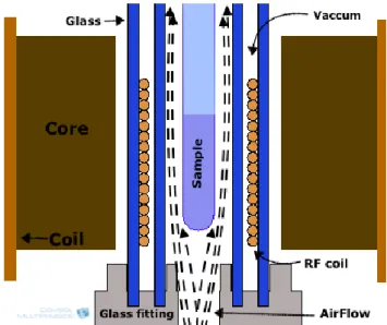
In principle, a field cycling NMR relaxometer has the typical configuration illustrated schematically in Fig. 1:
Fig. 1. Standard NMR spectrometer.
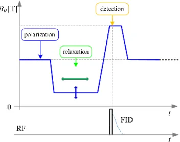
In a typical field-cycling NMR relaxometry experiment the sample is initially placed on a magnetic field, as high as possible, where it is polarized. This initial magnetic field is called polarization field, 𝑩𝟎𝑷. Typically, it is oriented
with the z axis, and forces the nuclear spin magnetization to be along , 𝑴⃗⃗⃗ = 𝑴𝒛𝒆⃗ 𝒛. Following this, the magnetic field
is switched down to a lower value 𝐵0𝐸. In this new applied
field, evolution field, the magnetization evolves to a new equilibrium, (𝑩𝑬) [2], [8].
The final stage of the cycle, is the detection stage. The magnetic field is again increased to a high value, 𝑩𝟎𝑫, with
sufficient homogeneity to allow NMR signal detection, along with a 𝜋
2 RF pulse, rotating the magnetization to the
xy plane. A recycle delay follows, where thermal equilibrium and polarization is reset, in order to begin the next cycle.
A field cycling example can be seen in Fig. 2.
Fig. 2. Typical cycle of the main magnetic field B0 [2].
Several cycles will occur with different parameters in order to observe the behaviour of the spin system.
As the sample has to experience different intensities of 𝐵0
field, there are two methods to achieve this. Mechanically moving the sample between positions of different magnetic fields, or to change the electrical current applied to the magnet in order to vary the intensity of the field. Despite the difficulties of achieving a short steady transition (3 – 100 ms) between fields, electronically switched field cycling is the only known alternative for measuring the shortest relaxation times.
3. The electromagnet – structure and
simulation
The core component of the FFC equipment is the electromagnet based on high permeability iron cores with a typical structure (Fig. 3). This geometry is composed by transformer E-shaped plates. This plates are piled together in order to avoid induced currents. The electromagnet consists on two symmetrical E plates brought together with a slight cut on each of the middle feet where the sample will be accommodated. The electromagnet's height is equal to the middle feet length in order to accommodate squared coils.
Fig. 3. Magnetic electromagnet with coils around the middle feet [9].
In order to define the electromagnet, a simulation using COMSOL Multiphysics® was performed.
Different physical quantities were susceptible to change influencing the characteristics of the spectrometer [2], [10]:
Ferromagnetic electromagnet: Different E-shaped transformer plates are available with different standard sizes, which is directly related with the electromagnet size and volume. The size of the electromagnet influence the magnetic flux density and maximum magnetic field. On one hand the smaller the electromagnet is the higher is the possible magnetic field, on the other hand the smaller is the available space for the coils limiting the number of turns and therefore the magnetic field;
Sample gap size: The smaller the gap the higher will be the magnetic field magnitude at the sample site but the smaller the height of the coils will be since they are inserted through the gap. There is a minimum limit since the sample need to be heated with air and a radio-frequency (RF) coil needs to involve the sample;
Maximum current applied to the coils: This is a crucial parameter since the magnetic field at sample site is directly related with the applied current. Joule heating effects must be considered as well as the fact that a higher magnetic field magnitude is created by higher currents;
Number of coils: Different number of coils can be accommodated in the electromagnet depending on its size. The more coil sets the electromagnet has the higher the magnetic field is but the other limitations might arise such as cooling ability and space;
Number of turns in each coil: This number should be as high as possible since it is directly related with magnetic field magnitude. It is limited by the gap size, length between E-plate feet, Joule loss effects and wire cross section.
After the evaluation of different electromagnet configurations the final decision was to built a spectrometer with the characteristics listed in Table I.
Table I. - Possible range of values for the simulation
Target Field 0.33 T
E-plate standard sizes 12/13.5/15 cm
Number of coils 6
Number of turns per coil [50 - 300]
Max. current in coils 5 A
Minimum gap size 15 mm
The magnetic field in the geometry was evaluated through the simulation [10]-[13], being crucial to analyse the homogeneity of the magnetic field (∆𝑩
𝑩𝟎). The typical flux
density and path is presented in Fig. 4.
Fig. 4. Top view of magnetic field plots: Volume and Arrow line. Designed in COMSOL Multiphysics® 4.3.
The homogeneity requirement arises from the fact that the sample needs to be polarized evenly by the same field magnitude in order for the RF pulse to match the Larmor frequency. This not only requires a uniform area in the sample site middle plane but a uniform volume. To further evaluate this volume, three planes in the air gap are analysed: the middle sample site plane (y=0) and two additional planes in y= ±0.35 cm.
The magnetic field magnitude in the center of the planes y=±0.35 cm must match the magnitude of the middle plane. Despite the divergence in magnetic field values in the limits of the section in both three planes the magnetic field magnitude converge to the 0.329 T.
To analyse the homogeneity, two square areas in each plane were defined: the inner square (2 cm x 2 cm), Ai and an outer square (4.5 cm x 4.5 cm), A0 that corresponds to the sample site section. For the y=0 plane the magnetic field is uniform in the centred square Ai with a magnetic field of 0.3288 T in the central point. The outer square A0 presents higher non-homogeneity since it is close to the sample site section limit and the fringing effect starts to become significant [14]-[17].
The same method is applied to the planes y=0.35 cm. In the y=0.35 cm plane the magnetic field presents a higher uniform in the centred square Ai with a magnetic field of 0.3289 T in the central point. The outer square A0 presents high non-homogeneity. In the y=-0.35 cm plane the magnetic field is also uniform in the inner square Ai with a superior uniform contour line than the y=0 cm case with a magnetic field of 0.3289 T in the central point. The outer square presents a quite different profile than the middle plane.
It is concluded that in the inner square (2 cm x 2 cm) exists high homogeneity in which each layer (y=0 has an homogeneity of 0.22%, y=0.35 cm of 0.01% and y=-0.35 cm plane of 0.03%) the magnetic field magnitude is By=0=0.3288 T, By=0.35=0.3289 T, By=-0.35= 0.3289 T. A difference in the magnetic field between the outer planes and the middle plane is observed (±0.0001 T). In the outer square the same cannot be observed and it becomes unnecessary to analyse the sample outside the inner square.
The mean values of the homogeneity are compared with the previous built equipment [9] in Table II. The homogeneity is proven to be acceptable with similar homogeneity results for the inner square and considerable better homogeneity in the outer square.
Table II. - Homogeneity values compilation along the FFC 3 [9] in the plane y =0 cm.
Section Case under study FFC 3 [9]
Ai 0.22% 0.20%
A0 22.94% 44.29%
4. Experimental testing of the electromagnet
Experimental confirmation of the physical quantities provided by the simulation and analytical calculations are desired.A. Electromagnet
In addition to the magnet structure described before, two additional coils were added to serve the purpose of auxiliary coils, which compensate permanent magnetizations of the electromagnet and the earth magnetic field. This coils are composed of 430 turns each with a copper wire of 0.25 mm diameter. The built electromagnet can be seen in Fig. 5.
Fig. 5. Specially developed electromagnet for a NMR FFC spectrometer: 4.5 cm height built of iron standard E shaped transformer plates 13.5 cm width, 1.5 cm gap in the middle foot, six coils with 218 turns each, maximum current of 3 A and maximum achievable magnetic field of 0.328 T.
B. Experimental measurements
Coil electrical resistance
The total resistance of the coils was measured in dc mode. The experimental resistance is 9.6±0.1 Ω compared to the 9.3 Ω theoretically calculated.
Coil Inductance
The inductance of the coils come as an important parameter to measure given its relation with the current variations necessary for field cycling. A direct measurement of the inductance was performed for all the six coils with an Inductance-meter that revealed: L=544.5±0.1 mH. The auxiliary coils both measured an inductance of Laux=134.2± 0.1 mH.
Another method was used to calculate the inductance L, as well as the leakage inductance LL, based on two combinations of coils: all six coils connected as usually (additive mode); and, in another case, half the coils fed by an opposite current in order to neutralize the field created by the other half (subtractive mode).
Using the AC current method an inductance of L=657.7 mH was obtained, and a leakage inductance of LL=229.36 mH which corresponds to 34.7% of the total inductance. Leakage flux is thought to arise from two factors: small electromagnet volume and proximity of the coils to the external feet. This proximity might prevent the lines to close properly and a higher distance would therefore reduce the fringing effect and leakage ratio. The first hypothesis was confirmed by the previously built electromagnet given the lower fringing ratio (1.62 against the 2.16 of the current work) [9].
To evaluate the impact of the proximity of the coils to the external feet a new fringing factor characteristic was calculated through data obtained by COMSOL MultiPhysics®. The original distance between internal and external feet is 2.25 cm, where only a few millimetres are left between the coil and the external feet. The new characteristic was calculated for a distance between feet of 5 cm which means a distance >2.75 cm between coils and external feet. The fringing ratio vs. gap size of the built electromagnet case (2.25 cm distance between feet), the 5 cm distance, and the previously built electromagnet (b=18 cm and distance between feet of 3 cm) is plotted in Fig. 6.
Fig. 6. Fringing ratio vs. gap size for the current case (2.25 cm distance between feet), the 5 cm feet distance, and the previously built electromagnet (b=18 cm with 3 cm distance between feet).
Both the fringing ratio and leakage flux present lower values for the 5 cm case than the current case. Despite the confirmation of the contribution of the feet distance to the fringing effect and flux leakage, Roque's characteristic reveals that the main contributor for the high leakage ratio is the volume of the electromagnet, [18].
C. Magnetic field magnitude measurement
The magnetic field magnitude over multiple planes vs. position was obtained through the simulation and evaluated. An experimental evaluation of the same kind was performed. The experimental set-up consisted in the magnetic electromagnet fed by a power supply, where both a ammeter and a voltmeter were embedded in the circuit in order to have a thoroughly evaluation of this physical quantities. A Hall Sensor (Model: GM-5180) was attached
to a XY Table which controlled its position along the desired area. All the measurements were performed with the coils under a DC current of 3 A.
The magnetic field magnitude was measured in a square with total area 9x9 cm2. This area involves the middle foot
section till the beginning of the outer feet. A measurement was performed every 5 mm for a fix xx axis, followed by an increase of 5mm in the yy axis. This resulted in a 17x17 grid and a total of 289 measured points.
The experiments allowed to confirm the range of fields around the electromagnet and the area where the fringing effect occurs confirming the predictions made by the simulation. The same process followed for the planes: y0=0 mm, y1=3.5 mm and y2=-3.5 mm.
From the measurements, the highest magnetic field point corresponds to the middle point of the middle plane (y0=0 mm): B0=0.3229 T.
The experimental data reveals similar expected homogeneity in the outer area, and relatively worst homogeneity in the inner area.
The volume of interest (sample placement) is the centred volume V1=2 x 2 x 0.7 cm3. The volumetric homogeneity in relation to the highest magnetic field (central point of the middle plane, B0=0.3229 T) is calculated by using the 25 point experimental points of each plane, which is 1.03%.
5. Coupled systems & spectrometer assembly
The electromagnet will operate inside a casing along with the remaining support systems which are: sample heating; cooling; RF coil.A. Sample heating
The spectrometer must be able to heat the test samples to temperatures up to 150 ºC. This is achieved by heated air and such system must be designed in order not to heat the electromagnet or other spectrometer components (Fig. 7). The air is heated by the use of a resistance in a tube. The acquired model is: Marathon-IN AH50050S.
The applied power is controlled by the power supply which uses a thermocouple placed close to the sample. This allows for a precise control of the sample temperature.
The specially designed component makes the hot air transition from a horizontal to a vertical flow. It also supports the next component: glass structure.
The glass structure is composed of two glass tubes. The inner tube has an inner and outer diameter of 8 and 9 mm, respectively. The outer tube has a 13 and 14 mm inner and outer diameter, respectively. The function of the glass is to guide the air towards the sample and supporting the sample (rounded tube up to 5 mm diameter), RF coil and thermocouple. The RF coil will be place in between tubes under vacuum. The goal of creating vacuum is to prevent heat transfer between the hot air and the spectrometer, and isolate the RF coil.
Connection tubes are required to connect the different components while assuring a rigid and reliable structure constituted by heat proof materials.
Pressurize air is injected into the spectrometer special valve which then leads the air to the heater, placed in the horizontal plane under the electromagnet. A connection valve - air heater is required. Another connection leads the heated air to the specially designed component forcing the flow from a horizontal to a vertical flow, into the glass structure. The glass structure where the sample is placed leads the air to exit the spectrometer through the top while heating the sample.
Fig. 7. Close up of the heating system. B. Radio Frequency Coil
The Radio Frequency (RF) coil allows for magnetization shifts and signal acquisition and is positioned in the center of the gap in the vertical plane. The Radio Frequency circuit is constituted by a coil and a capacitor which can both apply a RF pulse and receive NMR signals.
Despite the electromagnet is designed to reach a maximum magnetic field of B0≈0.33 T the current power supply is designed according to the previous versions of the FFC equipment’s. The Radio Frequency control system of the power supply is matched to the previous maximum magnetic field and Larmor frequency: 0.21 T and 8.862 MHz. This means that given the available power supply the electromagnet is required to operate at a maximum field of 0.21 T and the RF generator matched to a resonance frequency of 8.862 MHz.
The coil is placed around the inner edge of the outer glass tube. It is intended to use a 0.4 mm diameter wire for the coil with 2 cm length which require 50 turns.
The inductance of this coil calculated by [9]:
𝐿𝑅𝐹 = 𝑁2(𝑑2)2
9(𝑑2+10𝑙)≈ 15.2 𝜇𝐻 (1)
Where N is the number of turns, d the coil diameter and l the coil length. There are different possible configurations that can synchronize the RF circuit to a given frequency range being the one chosen a RLC circuit. The resonance of such circuit is given by:
𝝎𝒐=√𝑳𝑪𝟏 (4)
Where C stands for the capacitance. For an inductance of 15 µH and a desired resonance frequency of 8.862 MHz the capacitance is:
𝑪 =𝑳𝝎 𝟏
𝟎𝟐≈ 𝟐𝟏. 𝟐 𝒑𝑭 (5)
Two possible alternatives are possible to reduce the maximum magnetic field created by the electromagnet: by lowering the applied current to 2 A, or by removing two symmetrical coils (four coils should reach a magnetic field of B0 ≈0.22 T). Reducing the current is beneficial in terms of the Joule losses (from 84 W to 37 W). The removal of two symmetrical coils reduces the Joule losses (from 84 W to 60 W) but also allows for bigger distance in-between coils (facilitating air cooling) and increase the distance from coils to the electromagnet gap (favouring field homogeneity).
C. Cooling System
The cooling system relies on cold air flow to assure thermal stability of the electromagnet. A vertical flow is required through the middle of the electromagnet and two openings in the casing: inlet and outlet. This openings do not require to be horizontal as long as the air flow is forced into a vertical path. The vertical flow might require to perform a downward path given the positioning of the heating system. The heating system (positioned below the electromagnet) might heat the air significantly before it reaches the electromagnet compromising the cooling effects. This system is based on a fan that could be either axial or radial as long as their dimensions are small enough to fit the casing while being able to operate for long periods of time. D. Assembly
The electromagnet and coupled systems are intended to be assembled separately from the power supply. Currently the hypothesis of using a rectangular case of similar horizontal area as the electromagnet, but with additional height is under evaluation. The electromagnet is projected to be in the middle height of the case where the cooling system is placed above the electromagnet and the heating system and remaining systems under the electromagnet.
Openings in the case are required for air inlet and outlet. The inlet has the possibility to be in the top surface of the case or in upper lateral sides. For the outlet, openings in the bottom lateral sides are feasible as long as connecting wires are not in contact with the existing hot air. The horizontal area must be enough to correctly accommodate the heating system or extra space is necessary. An extra opening is necessary for sample insertion. The height of the case depends on the occupied volume by the heating system and cooling system. This relative positioning allows for the air to flow through the electromagnet, cooling it and the air heater ensuring thermal stability of all the components. The power supply and pressurized air connections are to be made in the back of the spectrometer and accommodated in the bottom of the spectrometer.
6. Final Remarks
A small FFC NMR magnet with high homogeneity in the sample site is achieved and is designed to operate within the magnetic field range of 0 and 0.33 T. Thermal effects and cooling requirements were evaluated allowing for the projection of feasible systems. The computational simulation allowed to estimate air flow rates for safe measurements over extended periods of time. The sample heating system was projected and some components acquired and defined. The sample heating system projection allowed the definition of the RF circuit and specific coil and capacitor parameters were defined which guarantees NMR resonance conditions.
The advantages of the developed FFC magnet relatively to the generality of magnets are: reduced electromagnet's volume and weight, low power consumption, high homogeneity profile, feasible and low power cooling system.
Acknowledgement
This work was supported by national funds through Instituto Politécnico de Setúbal, ISEL/Instituto Politécnico de Lisboa, Fundação para a Ciência e a Tecnologia (FCT) with reference UID/CEC/50021/2013
and UID/CTM/04540/2013.
References
[1] M. Levitt, “Spin Dynamics: Basics of Nuclear Magnetic Resonance”, Wiley, 2001.
[2] F. Noack, “NMR Field-Cycling Spectroscopy: Principles and Applications”, Prog. NMR Spectrosc., 1986, 18, pp. 171-276. [3] R. Kimmich and E. Anoardo, “Field-Cycling NMR relaxometry”,
Progress in NMR Spectroscopy, 2004, 44, pp. 257-320.
[4] E. Anoardo, G. Galli, G. Ferrante, “Fast-Field-Cycling NMR: Applications and Instrumentation”, Applied Magnetic Resonance, 2001, 20, (3), pp. 365-404.
[5] R. Seitter, R. Kimmich, “Magnetic Resonance: Relaxometers”, in Encyclopedia of Spectroscopy and Spectrometry (Academic Press, London, 1999), pp. 2000-2008.
[6] D. M. Sousa, G. D. Marques, J. Cascais, J. Sebastião, “Desktop Fast-Field Cycling Nuclear Magnetic Resonance Relaxometer”, Solid State Nuclear Magnetic Resonance, 2010, 38 (1), pp. 36-43. [7] D. M. Sousa, G. D. Marques, P. Sebastiao, and A. Ribeiro, “New
isolated gate bipolar transistor two-quadrant chopper power supply for a fast field cycling NMR spectrometer”, Review of Scientific Instruments, 2003, 74 (3), 4521-4528.
[8] A. Abragam, “The Principles of Nuclear Magnetism”, Oxford University Press, London, 1978.
[9] A. Roque, “Espectrómetro de RMN de CCR com utilização de supercondutores no magneto” PhD thesis, Instituto Superior Tecnico, Universidade de Lisboa, 2014.
[10] M. Sciandrone et al., “Compact low field magnetic resonance imaging magnet: Design and optimization”, Review of Scientific Instruments, VOL. 71, no. 3, March 2000.
[11] A. E. Umenei et al., “Models for Extrapolation of Magnetization Data on Magnetic Cores to High Fields”, IEEE Transactions on Magnetics, VOL. 47, No. 12, December 2011.
[12] S. Hahn et al., “Bulk and Plate Annulus Stacks for Compact NMR Magnets, Trapped Field Characteristics and Active Shimming Performance”, IEEE Transactions on Applied Superconductivity, VOL. 23, NO. 3, June 2013.
[13] A. Roque, S. Ramos, J. Barão, V. M. Machado, D. M. Sousa, E. Margato, J. Maia, “Simulation of the Magnetic Induction Vector of
a Magnetic Core to be used in FFC NMR Relaxometry”, J. Supercond. Nov. Mag., Vol. 26, Issue 1, Page 133-140, 2013. [14] C. W. T. McLyman, “Tranformer and Inductor Design Hanbook”,
Second Edition, Marcel Dekker, 1988.
[15] A. Roque, D. M. Sousa, E. Margato, J. Maia, G. Marques, “Characterization of the Fringing Window of a Magnetic Core”, EUROCON, IST, Lisboa, 2011.
[16] J. Fletcher, B. Williams and M. Mahmoud, “Air gap flux fringing reduction in inductors using open-circuit copper screens”, IEE Proc.-Electr. Power Appl., Vol. 152, no. 4, pp. 990-996, July 2005. [17] R. J. Weggel and C. F. Weggel, “High-Homogeneity NMR and MRI
Magnets With Minimized Fringe Field”, IEEE Transactions on Applied Superconductivity, Vol 24, no. 3, June 2014.
[18] A. Roque, D. M. Sousa, E. Margato, V. M. Machado, P. J. Sebastião and G. D. Marques, “Magnetic Flux Density Distribution in the Air Gap of a Ferromagnetic Core With Superconducting Blocks: Three-Dimensional Analysis and Experimental NMR Results”, in IEEE Transactions on Applied Superconductivity, vol. 25, no. 6, pp. 1-9, Dec. 2015.
![Table II. - Homogeneity values compilation along the FFC 3 [9]](https://thumb-eu.123doks.com/thumbv2/123dok_br/15565707.1047417/4.892.73.426.588.772/table-ii-homogeneity-values-compilation-ffc.webp)