E↵ects of stellar activity on the
measurement of precise radial velocity
Departamento de F´ısica e Astronomia
Faculdade de Ciˆencias da Universidade do Porto
E↵ects of stellar activity on the
measurement of precise radial velocity
Tese submetida `a Faculdade de Ciˆencias da Universidade do Porto para obten¸c˜ao do grau de Doutor
em Astronomia
Departamento de F´ısica e Astronomia Faculdade de Ciˆencias da Universidade do Porto
I would like to thank my supervisor, Nuno, the motivation, patience, guidance, and scientific expertise he shared with me, and for all the work he had to make this thesis a reality. I would also like to thank all my co-workers and staff at CAUP for helping me with the scientific and bureaucratic aspects of the PhD, but also for the fun we had in innumerable occasions during these last four years. And of course to all my friends and family.
This research was funded by Fundac¸˜ao para a Ciˆencia e Tecnologia, Portugal (grant ref-erence SFRH/BD/64722/2009) as well as by the European Research Council/European Community under the FP7 through Starting Grant agreement number 239953.
The radial velocity (RV) method is one of the most prolific techniques in detecting and confirming extrasolar planets. However, due to its indirect nature, it is also sensitive to other sources of RV signals. One of the most important limiting factors of using the RV method to discover low-mass or long-period extrasolar planets is stellar activity. The phenomena that comprises activity is capable of inducing ”artificial” RV variations that will interfere with planetary detections, by adding noise to the data or producing periodic modulations that might be confused with the ones originating from the pull of planetary companions. These phenomena have a large range of timescales, from stellar oscillations and flares that can last for minutes, to magnetic cycles that last for decades. When searching for planets with various orbital periods, all these timescales need to be taken into account. Therefore, it is very important to understand the activity diagnostic tools and how activity interferes with the measured RV.
In this thesis my focus is on the long-term interference of activity on the measured RV signals and how to diagnose them. A large part of the work involved studying activity cycles of M dwarfs, due to their increasing importance in planetary searches, mainly because of their low-mass, which maximises the detection of planets by using methods such as RV or transits. I compared various activity indicators measured over timescales of years to try to understand how they relate to each other and select the most appropriate for these kind of stars. The flux in the Na i D lines was found to follow very well the activity measured by the Ca ii H & K lines. Furthermore their use is most appropriate for M dwarfs due to the higher signal-to-noise at the Na i D wavelengths. I also found that the flux in the Ca ii and H↵ lines is correlated for the highest activity stars but uncorrelated or anti-correlated for he most quiet M dwarfs. Indications that activity cycles are present in early-M dwarfs were also detected.
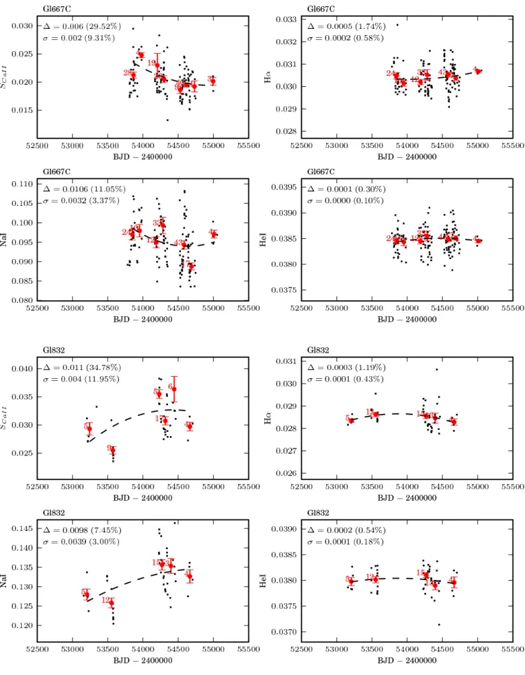
In a following study with one more year of extended data, the flux on the Na i lines was used to detect activity cycles and compare those variations with the simultaneous RV signals. This was done with the aim of finding correlations between activity and RV and
long-term variability is comparable to that of FGK stars. However, only 19% of early-M dwarfs show the presence of activity cycles (cf. ⇠60% for FGKs). This might be a signal of departure from an ↵⌦-dynamo to an ↵2-dynamo were no activity cycles are expected. I also found that long term activity variations are capable of producing RV signals with amplitudes that can reach the ⇠5 m s 1 level. This is enough to hide the signal of a low-mass planet or to simulate that of a long-period planet.
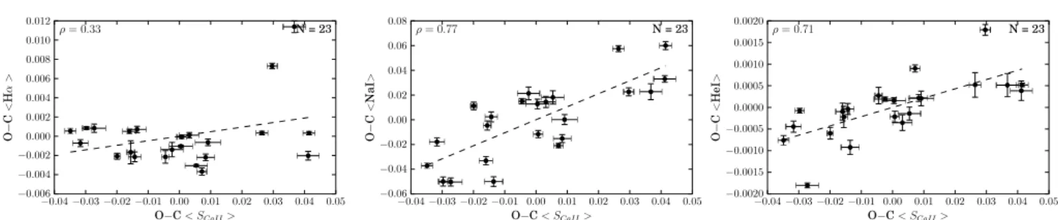
In the last part of this thesis I studied the long-term correlation between two of the most widely used optical activity indicators, the Ca ii H & K and the H↵ lines, for a sample of FGK stars. These two indices are known to have a wide range of correlations but this behaviour is not well studied. The correlations between these indices was found to be depend on the activity level of the stars (as was found also for M dwarfs) and the stellar metal content might be also having an effect on the correlations between these two activity indices.
Acknowledgments 3
Abstract 4
List of Tables 8
List of Figures 9
1 Introduction 10
1.1 Detecting exoplanets using radial velocity . . . 12
1.1.1 General properties of exoplanets . . . 13
1.1.2 The radial velocity method . . . 16
1.1.3 Limitations of the radial velocity method . . . 18
1.2 Stellar activity . . . 19
1.2.1 Stellar chromospheric activity . . . 20
1.2.2 Activity proxies . . . 25
1.2.3 Mean activity level of stars . . . 30
1.3 Stellar activity at different time scales and its influence on RV . . . 32
1.3.1 Oscillations and Granulation . . . 32
1.3.2 Rotationally modulated active regions . . . 36
1.3.3 Long-term activity: magnetic cycles . . . 38 6
2 Long-term magnetic activity of a sample of M-dwarf stars from the HARPS
program I. Comparison of activity indices 45
3 Long-term magnetic activity of a sample of M-dwarf stars from the HARPS
program II. Activity and radial velocity 63
4 On the long-term correlation between the flux in the Ca ii H & K and Halpha
lines of FGK stars 89
5 Conclusions 108
5.1 Activity indices for M dwarfs . . . 108 5.2 Long-term activity variability and cycles of M dwarfs . . . 110 5.3 Influence of long-term activity on the RV of M dwarfs . . . 111
5.4 The long-term correlation between Ca II and Halpha for FGK stars . . . 112
5.5 Future prospects and things to be done . . . 113 5.5.1 Activity cycles in M dwarfs . . . 114 5.5.2 Activity indices . . . 115
References 116
1.1 Stellar activity at different timescales and correction of RV. . . 33
1.1 Mass distribution of close-in, low-mass planets . . . 14
1.2 Radius distribution of low-mass planets . . . 15
1.3 Solar flare . . . 21
1.4 Temperature structure of the solar chromosphere . . . 23
1.5 RV induced by stellar oscillations . . . 34
1.6 Effect of granulation on line bisector . . . 35
1.7 Effect of spots on line profile and RV . . . 37
1.8 The Sun’s butterfly diagram and average sunspot area . . . 39
1.9 MWO long-term activity classification . . . 40
1.10 Long-term correlations between RV and activity proxies . . . 42
Introduction
During the last 15 years, astronomers have been discovering dozens of planets orbiting other stars. This quest is, however, not an easy task. The difficulty of detecting extra-solar planets arises from the fact that most of the optical radiation coming from a planet is simply reflected starlight. Because of this, exoplanets will be billions of times fainter than their host stars. And since they generally orbit at extremely small angular separations, their direct detection is incredibly hard. One way to circumvent this problem is to use indirect methods such as detecting the dynamical perturbations provoked in the host star by a planetary companion.
Several indirect methods exists now that are able to detect these small bodies in other stellar systems. The most successful to date are the radial velocity (RV) method, one of the focus of this thesis, which measures the line-of-sight velocity of star as it moves around of the star-planet centre of mass (e.g. Mayor & Queloz 1995), and transit pho-tometry which detects the shallow brightness decrease of a star as a planet passes in front of its disk (e.g. Henry et al. 1999; Charbonneau et al. 2000). Other indirect methods currently in use include astrometry, which measures the apparent movements of the parent star by measuring it’s position with time (e.g. Benedict et al. 2006), gravitational microlensing events, which detects the huge jump in the brightness of a planet as a lens star passes in front of its host star (this method is however not easily repeatable) (e.g. Bond et al. 2004). Transit timing variations, which measure the variations in the transit time of a planet produced by another perturbing body (e.g. Ballard et al. 2011), is recent new method for confirming or detecting exoplanets. Another example of an indirect planet search technique is pulsar timing, which measures the tiny anomalies in the timing of its observed radio pulses and can be used to track the pulsar’s motion, and therefore to detect a perturbing companion (e.g. Wolszczan & Frail 1992). This last
one was the technique that first detected planet mass objects outside the solar system Wolszczan & Frail (1992).
Due to the indirect nature of these methods, they will become sensitive to other sources of signals, similar to the ones they are supposed to detect, which can be produced by the parent star. In this thesis I am more concerned with the RV method. Activity perturbations in the stellar atmosphere, stellar oscillations, surface granulation, and magnetic activity cycles, can all perturb the observed RV to different scales in terms of time and amplitude. These effects might make the detection of exoplanets extremely difficult, by hiding their signal in the stellar noise or by producing periodic signals that can be confused with the ones of real orbiting planets (e.g. Queloz et al. 2001).
The study of these stellar activity sources of noise is the main aim of this thesis, in particular the long-term activity variations of solar-type stars and M dwarfs and the way they influence a star’s RV. A first step in the understanding of how activity affects RV is to first know how to interpret the activity diagnostics. Different activity indicators will trace different activity phenomena, which will affect the RV in different ways. And by understanding precisely which are the effects of each activity phenomena and how to correct them, a higher RV precision might be attained. If the true RV signals of real planets can be effectively disentangled from stellar RV noise, then the path is open for first detection of an Earth twin.
The organisation of this thesis is the following. I start by introducing the topic of ex-trasolar planet search using the radial velocity method in section 1.1 where I give a brief summary of the occurrence and main properties of the exoplanets detected so far (sect. 1.1.1), then describe the fundamentals of the method (sect. 1.1.2) and its main limitations (sect. 1.1.3). I then move to the subject of stellar activity in section 1.2. Here I discuss what is stellar activity, a chromosphere, and what produces them, what stars have activity and chromospheres and why stellar activity is important for exoplanet research (sect. 1.2.1). I also describe the distribution of the activity levels of stars, the connection between mean activity level and other stellar parameters and the influence of activity on RV in general terms (sect. 1.2.3). Then I move to the field of activity detection, where I give a small description of the most common activity diagnostics in use (sect. 1.2.2). Finally, I go through all the timescales of the different activity phenomena, how they affect RV and describe some ways to correct or minimise their effects (sect. 1.3). The motivation of this thesis is presented in the end of this chapter (sect. 1.4). In chapters 2, 3, and 4, I present the results of this work in the form of three peer-reviewed papers. Finally, in chapter 5 I conclude by discussing the results of this thesis and giving some future prospects.
1.1 Detecting exoplanets using radial velocity
The first confirmed planet orbiting another solar-type1 star was the famous 51 Peg b discovered by Mayor & Queloz (1995). It is a giant planet with a mass of 0.47 MJ and orbiting extremely close to its parent star, with an orbital period of just 4.2 days. Other two massive planets were rapidly announced in the same year following this first discovery (Marcy & Butler 1996; Butler & Marcy 1996). This realisation that planets orbiting other stars existed accelerated this new field in astronomy and the discovery of planets in other stellar systems has now become routine.
To date, 531 planets were confirmed via the radial velocity method (also known as Doppler spectroscopy). This includes 399 planetary systems where 93 are multiple-planet systems2. The first discovered planets were very massive and orbiting their parent stars on short period orbits. Jupiter mass planets in close orbits or very eccentric planets were not expected configurations from theories of giant-planet formation based on the only stellar system that we had known for millennia (Pollack et al. 1996). Differ-ent theories have appeared which explained these new configurations, as for example that massive exoplanets are formed far from the star and then migrate to their current positions (e.g. Lin et al. 1996; Trilling et al. 2002). However, more recently, giant planets much more similar to the solar system giants (e.g. Wright et al. 2008; Boisse et al. 2012) along with smaller mass planets with sizes closer to that of rocky planets have been detected (e.g. Udry et al. 2007; Mayor et al. 2009; Dumusque et al. 2012). This was a result of improved spectrograph precision (for example, HARPS3 can now reach below 1 m s 1precision, Pepe et al. 2005), observational strategies capable of removing RV noise caused by stellar oscillations (Santos et al. 2004; Dumusque et al. 2011b), and increased timespan of observations which will enable the easier detection of lower-amplitude signals immersed in noise or add enough data to detect the long-period planets.
1The first extrasolar planet detected by the radial velocity method was a 1.7 MJmass planet with a period
of 2.7 yr around Cep announced by Campbell et al. (1988). However, this planet would need to wait almost two decades before being confirmed (Hatzes et al. 2003).
2From http://exoplanet.eu/, (Schneider et al. 2011).
3HARPS (High Accuracy Radial velocity Planet Searcher, Mayor et al. 2003) is a high-resolution
1.1.1 General properties of exoplanets
Since the focus of this thesis is on planet detection (by studying the limiting factors), I will describe very briefly some of the basic properties and planet occurrence rates obtained from some important planet search surveys.
Close-in, low-mass planets Contrarily to what can be found in our solar system, planets of intermediate sizes between Earth and Neptune are very common in other stellar systems. They also appear to outnumber the larger sized planets at close-in orbits (Howard et al. 2010; Mayor et al. 2011).
The results from the Eta-Earth RV Survey (166 G and K-type stars) shown that 15% of Sun-like stars host at least one low mass planet with Msin i = 3-30 MEarth in orbits closer than 0.25 AU (P < 50 days) and that, by extrapolation of the power law fitted to their data, another 14% of stars host planets with Msin i = 1-3 MEarth (Howard et al. 2010).
On it’s hand, the HARPS RV survey of 376 FGK stars shown that more than 50% of the solar-type stars harbour at least one planet of any mass at short orbital distances with P < 100 days (Mayor et al. 2011). For the case of low-mass planets, this survey found that the mass distribution of super-Earths and Neptune-mass planets (with P <50 days) strongly increases between 30 and 15 MEarth. The orbital eccentricities of these type of planets are generally low, with e values lower than 0.45. No correlation between the occurrence rate and host star metallicity was detected. In this survey, it was also demonstrated that low-mass planets are normally found in multi-planet systems with 2-4 small planets with orbital periods of weeks or months.
These two surveys showed that the occurrence of low-mass and close-in planets in-creases with decreasing mass (see e.g. Fig. 1.1).
The Kepler transit survey increased the number of detected low-mass candidate planets to the thousands. As can be observed in Fig. 1.2, the distribution of planetary sizes follows a similar pattern as the mass distribution where the frequency o planets rises with decreasing planetary radii (Howard et al. 2012; Petigura et al. 2013; Fressin et al. 2013). However, the increase in occurrence with decreasing radii stagnates at ⇠2.8 REarth and becomes roughly constant for smaller radii (Petigura et al. 2013). This means that it is as common to find an Earth-sized planet within 0.25 AU as to find a Super-Earth with twice the Super-Earth’s size. As was found for the mass distribution, the smaller-size planets detected by Kepler appear to have less eccentricity than larger planets
Figure 1.1: Mass distribution of close-in, low-mass planets with periods P < 50 days. Black line is the observed histogram and red line the equivalent histogram after correction for the detection bias. From Mayor et al. (2011).
(Plavchan et al. 2012). An interpretation of this can be that these planets suffer reduced dynamical interactions (Howard 2013). Twenty three percent of the Kepler stars host two or more transiting planets (Burke et al. 2013).
Regarding low-mass planets orbiting M-dwarfs, the HARPS M-dwarf survey found that super-Earths (Msin i = 1–10 MEarth) are relatively common around these stars (Bonfils et al. 2013). Around 36% of M-dwarfs host a super-Earth with an orbital period between 1 and 10 days, while 52% host a super-Earth with a period between 10 and 100 days.
Gas giant planets These planets are the easiest to detect, both by the radial velocity method and the transit technique. Observations taken at the Keck Observatory have shown that 10.5% of G and K-type stars host at least one giant planet with masses between 0.3 and 10 MJupiterin orbital periods in the range 2-2000 days (⇠0.03-3 AU) and that the occurrence rate of giant planets increases with increasing orbital distance and decreasing mass (Cumming et al. 2008). By extrapolation of the giant planet distribution, 17-20% of the solar-type stars harbour giant planets orbiting within 20 AU (P ⇠ 90 yrs,
Figure 1.2: Radius distribution of low-mass planets. The red line is the power law fitted to the histogram. From Howard et al. (2012).
Cumming et al. 2008). This is consistent with the detection of giant planets at longer distances than ⇠2 AU by microlensing surveys (Gould et al. 2010).
The HARPS survey found similar results. About 18% of solar-type stars have a planetary companion more massive than 50 MEarthon an orbit with a period shorter than 10 years and the occurrence rate of giant planets grows with the logarithm of the period. They also found cases of orbital eccentricities of gas giants higher than e =0.9 (Mayor et al. 2011).
There is a tendency for orbital distances of giant planets to be larger than ⇠1 AU however there is also a small pile-up at very short distances from the stars, near ⇠0.05 AU, the so called ”hot Jupiters” (see e.g. Udry et al. 2003; Howard 2013). These two populations of giant planets are thought to be the result of different migration scenarios acting during the planet’s evolution (see e.g. Udry et al. 2003). For the case of multi-planet systems, the orbital distribution is more homogeneous: there is no pile-up of hot Jupiters and now increase of occurrence with increasing distance after ⇠1 AU.
The giant planet eccentricity is different between single-planet and multi-planet systems: single planets show higher eccentricity rates than the planets in multi-planet systems (e.g. Howard 2013). This can be a result of planet-planet scattering processes in action as shown by Chatterjee et al. (2008).
The frequency of hot Jupiters (giant planets with P 10 days) is not as high as for other types of planets. The California Planet Survey from the Lick and Keck planet searches estimated that only 1.2% ± 0.38% of Sun-like stars host such a planet (Wright et al. 2012). A similar occurrence rate of 0.9% for hot Jupiters with M 50 MEarth and P 11 days was also found by the HARPS survey (Mayor et al. 2011). Contrarily to close-in low-mass planets, hot Jupiters are not commonly found close-in multiple-systems (Steffen et al. 2012). There is also a tendency for low eccentricity among these planets due to tidal circularization (Marcy et al. 2005).
The HARPS M-dwarf survey also found low occurrence rates for giant planets orbiting these small stars (Bonfils et al. 2013). For orbital periods between 1 and 10 days, this survey estimated that less than 1% of M-dwarfs host a planetary companion with a mass between 100 and 1000 MEarths, which is an occurrence rate comparable with that of the hot Jupiters for FGK stars. For longer periods, between 10 and 100 days, this frequency increases to around 2%.
1.1.2 The radial velocity method
A very significant part of the exoplanets discovered until now, were detected by the radial velocity (RV) method (also known as Doppler spectroscopy). This technique measures the movements of a star when pulled by an orbiting companion. These movements will produce a periodic variation in the wavelength of the stellar spectrum (the Doppler effect) which are due to the change in direction of the radial velocity of the star. This variation in wavelength is related to the RV of the star vie the Doppler Effect equation:
0 ' Vr
c , (1.1)
where = 0 is the change in wavelength due to the star’s motion, 0 the rest
wavelength of the spectral line, Vr the radial velocity (measured along the line-of-sight), and c the speed of light in the vacuum.
During the movement around the centre of mass, when the star starts moving away from the observer, its radial velocity becomes positive and the spectrum is shifted to higher wavelength values (light is redshifted, Vr > 0, >0). When the star is approaching the observer, the measured radial velocity is negative and the spectrum is shifted towards lower wavelengths values (light is redshifted, Vr > 0, > 0). These periodic redshifts and blueshifts in the spectrum will translate into a periodic RV signal in the case of a planet moving on a edge-on circular orbit.
The radial velocity method is based in the measurements of the Doppler shift of spec-tral lines. However, there are stellar phenomena that distorts line profiles and induce artificial Doppler shifts in the measurements, which are then translated into RV noise (a discussion of stellar noise is presented in section 1.2.1). After this type of noise is taken into account, the residual radial velocity will be the signal induced by the orbiting planet. From this signal, some planetary orbital and physical parameters can obtained.
The RV signal of a star having a planet moving in a non-perturbed keplerian orbit is of the form
Vr(t) = K[cos(⌫(t) + !) + e cos(!)] + (1.2)
where K is the velocity semi-amplitude,
K = 2⇡a?sin i
P(1 e2)1/2, (1.3)
where a?is the star’s orbital semi-major axis, i the orbital inclination, ! is the longitude of periastron, and is the systemic velocity (velocity of the barycentre). The true anomaly, ⌫(t), depends on the orbital period (P), eccentricity (e) and time of passage at periastron (T0). Therefore, fitting a radial velocity time series with this keplerian model yields six parameters: K, e, !, T0, P, and . The velocity semi-amplitude is related to the masses of the two components through the mass function,
(mpsin i)3 (m?+mp)2 =
P
2⇡GK3(1 e2)3/2 (1.4)
where mp is the mass of the planet, m? the mass of the star, and G the gravitational constant. The right-hand-side parameters of this equation can be obtained by the fit of the RV function. When assuming that mp ⌧ m?, Eq. 1.4 reduces to the expression of the planet minimum mass
mpsin i '✓ P 2⇡G
◆1/3
Km2/3? (1 e2)1/2. (1.5)
Only the minimum mass, mpsin i, can be obtained by this method since the inclination, i, is not known. An expression for the semi-major axis of the relative orbit can be obtained by applying the same approximation as before to the Keplers third law,
a ' ap' ✓ G 4⇡2
◆1/3
m1/3? P2/3. (1.6)
Therefore, fitting radial velocity data with a keplerian model to account for the presence of a planetary companion gives four of the six orbital elements of the relative orbit (the
longitude of the ascending node, ⌦, and the orbital inclination, i, remain unknown). Note however that not knowing the inclination is not statistically relevant. If inclination angles are isotropically distributed, then edge-on orbits are a lot more frequent than face-on systems. Therefore, systems with sin i > 0.5 will have a probability of about 87% (see Lovis & Fischer 2011).
By estimating the mass of the central star using other techniques, the keplerian fit will deliver a lower limit of the companion’s mass together with the semi-major axis of the relative orbit. Although, only the orbital parameters and a lower limit on the mass are known from radial velocity measurements, when combined with transit photometry, the true mass, radius and, consequently, the mean planetary density can be estimated. For a planet in a circular orbit around a solar-mass star, Eq. 1.5 simplifies to
K [m s 1] ' 28.57 m
psin i [MJup] P 1/3 [yr]. (1.7)
Since the probability of detecting a planetary signal depends in a first approximation on the value of the velocity semi-amplitude, this expression indicates that radial-velocity measurements favour the detection of planetary systems with massive and short-period planets. As an example, the radial velocity semi-amplitude induced by Jupiter and Earth on the Sun is 12.4 and 0.09 m s 1, respectively.
A very high-precision of below 1 m s 1 can be achieved, for example, via the cross-correlation function (CCF), which uses information from several thousand lines that are averaged into a single line profile, whose centroid is then used to determine de RV (e.g. Baranne et al. 1996).
1.1.3 Limitations of the radial velocity method
As was stated before, the radial velocity technique is one of the most successful method for detecting (and confirming) exoplanets. However, it was not until this technique was able to reach the high-precision required to detect RVs of several tens of m s 1when the exoplanet search by RV became so successful. To achieve this, wavelength calibration of the observed spectrum became a crucial step in data processing. Wavelength cali-bration data was included in the target spectrum with the aim of directly detecting any instrumental effects during the observations. Two main methods have been applied: the calibration lamp or the absorption sell. The first uses a calibration source next to the target spectrum which will be compared with the stellar spectrum (e.g. the ”ThAr method”, see Pepe et al. 2002) while the other uses an absorption cell in front of the spectrograph, which will imprint a dense forest of absorption lines from the cell onto
the spectrum (e.g. the ”iodine cell”, see Butler et al. 1996). By using either of these methods, any systematic effect in the wavelength solution of the spectrum will be directly monitored at the time of observations.
Note however that the stars themselves (and stellar properties) can affect the precision that can be achieved by the RV method. One such example is stellar rotation. Stellar rotation will broaden the spectral lines, which, in the case of fast rotating stars, would blend with neighbouring lines and reduce the attainable precision of RV (Bouchy et al. 2001). To minimise this, planet search surveys normally discard fast-rotators from their samples, which includes young stars and early-types.
The RV method can now achieve a precision better than 1 m s 1 (Pepe et al. 2011),
enabling the detection of planets with masses close to that of Earth (Mayor et al. 2009; Dumusque et al. 2012). At these levels of precision, one of the major limitations of the RV method comes from the RV ”noise” produced by stellar intrinsic variability. Stellar magnetic activity in the form of spots, plages, changes in the convection pattern, and others, can cause RV noise which can be easily detected by high-precision spectro-graphs. As an example, a spot covering 0.5% of a solar-type star will induce an RV signal of around 0.5 m s 1 (Saar & Donahue 1997; Hatzes 2002), totally hiding the signal produced by an Earth-like planet around a solar-like star (which is around 0.09 m s 1). The knowledge of how stellar activity behaves in different stars, the connection between all the activity phenomena and RV, and finding methods to correct or minimise them, is then of extreme interest for the quest of finding another Earth orbiting in the habitable zone of another star. In the following section I will discuss the magnetic activity phenomena of other stars, always keeping the exoplanet search subject in mind.
1.2 Stellar activity
Stellar activity is what we call the phenomena produced by the presence of magnetic fields in the atmosphere of cool stars. Variations in the magnetic fields topology affects all atmospheric layers of a star ranging from the cool photosphere up to the hot corona (see e.g. Hall 2008). These variations can be observed on a large range of timescales, from minutes to years (e.g. Baliunas et al. 1995; Dumusque et al. 2011b). For example, stellar flares are magnetic bursts in the atmosphere which normally causes huge vari-ations in the brightness and spectrum of a star with a duration of seconds to minutes. On longer timescales, stellar activity cycles, like the 11 year cycle of our Sun, are the product of changes in the global magnetic configuration, and have cyclic variations that
can range from months to a few decades.
The activity phenomena induced by stellar magnetic fields is thought to be produced by dynamo processes in the stellar interior which is linked to the star’s rotation and age, in solar-type stars.
The study of stellar activity is important to understand the structure and evolution of stars and the interstellar medium but also to exoplanet search and characterisation, since activity interferes with the most used exoplanet detection methods, Doppler spec-troscopy and transit techniques, and can also affect the weather and habitability of orbiting planets (see e.g. Buccino et al. 2006; Kaltenegger et al. 2010). In this work, we are mostly focused in studying the long-term activity variations of cool stars and the effects of stellar activity on the observed radial velocity.
In this section, we will discuss stellar chromospheric activity, how does it arises and which stars have it (sect. 1.2.1), the mean activity levels of stars and correlations with stellar parameters and RV (sect. 1.2.3), how to detect it and the mostly used activity proxies (sect. 1.2.2), the different timescales of activity, how they affect RV, and ways to limit the interference of activity in the detection of exoplanets (sect. 1.3).
1.2.1 Stellar chromospheric activity
The Sun, and similarly other solar-type stars, have the core in its centre, where nuclear fusion generates the energy. Surrounding the core there is a layer, the radiative zone, where the energy generated in the core is carried outward in the form of energetic photons via electromagnetic radiation. This radiative layer extends up to around 70% of the solar radius. Above, and extending up to the surface, is the convection zone where energy is transferred from the radiative zone to the solar ”surface” by convection: heated matter rises to the surface and, as it cools, its density increases and it sinks back down. This phenomenon results in the structure called granulation, where the bright granules, the regions where hot plasma is rising to the surface, are surrounded by darker boundaries, where cooler plasma is sinking down (e.g. Dravins et al. 1981). The solar disk that we see with the naked eye, and which is generally called the ”surface”, is the photosphere, which lies at the outer edge of the convection zone.
Above the photosphere, is the Sun’s atmosphere which extends itself into interplanetary space. The atmosphere is characterised by an extremely low density when compared with the solar interior. The main regions of the solar atmosphere are the inner
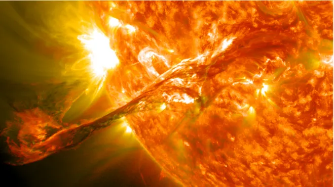
chro-Figure 1.3: A solar flare representing the solar atmosphere as a dynamic environment. Pictured here is a lighten blended version of the 304 Å and 171 Å wavelengths. Credit: NASA Goddard Space Flight Centre.
mosphere and the outer and more extended corona. The chromosphere is just a few thousand km in extension. After dropping from around 15 · 106 K in the core to around 5800 K in the photosphere, the temperature of the solar chromosphere increases from 4300 K just above the photosphere to around 50 000 K below the corona. At the transition region between the chromosphere and the corona, the temperature jumps from around 800 000 K to 3 · 106 K. For the solar atmosphere, with its low density, to increase so much in temperature, heating mechanisms other than the ones acting in the solar interior are needed.
In a stellar atmosphere in radiative equilibrium (RE), the energy is transported through the plasma via radiation. In this scenario, the heat absorbed from the radiation field and the thermal emission of the plasma are balanced so that the outward flow of energy from the deep interior is maintained. The outward temperature rise observed in the chromosphere can occur under specific conditions in RE (e.g. Auer & Mihalas 1969; Skumanich 1970). However, since emission reversals in prominent lines such as Ca II H and K are known to be signs of departures from RE (Hall 2008), other means of heating are necessary to explain the additional radiative losses in these and other lines. The effects these mechanisms of heating have in a stellar atmospheres are what is generally called activity (Hall 2008).
In the Sun and other solar-type stars, there are phenomena that deposit mechanical energy into the atmosphere covering the photosphere. This dumping of energy causes heating beyond the expected RE values for the increasingly tenuous plasma. The increase of energy in the plasma can be balanced by increasing hydrogen ionisation as it warms from ⇠5000 K to ⇠8000 K, which sets free a large supply of electrons that allows the collisional radiative cooling of the chromosphere. However, as soon as the hydrogen reservoir becomes fully ionised, the plasma loses this essential cooling mechanism and the temperature jumps from chromospheric to coronal temperatures. The chromosphere is not an homogeneous layer. On the other hand, it is variable on the short and long timescales, and characterised by regions of hot plasma which suggest a complex magnetic topology. For example, there are tightly collimated jets of plasma streaming upward through the chromosphere, spicules and macrospicules (Roberts 1945; Bohlin et al. 1975), which are bright in H↵ and gives the chromosphere its orange colour. Furthermore, dark regions of cool gas with sub-photosphere temperatures (< 4000 K) are also observed in the chromosphere layer (Solanki et al. 1994).
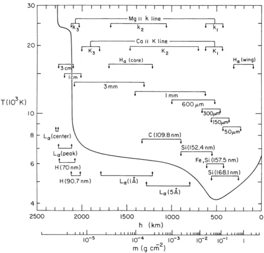
Numerous definitions of chromosphere have been proposed, based on height, temper-ature, physical processes, or some combination of these. Figure 1.4, shows the early model of the solar chromosphere produced by Vernazza et al. (1981). In this model, the chromosphere would be a layer ranging from 500 km to around 2200 km above the photosphere. In this region the temperatures start with the minimum temperature of ⇠4400 K in the lower chromosphere, then slowly rise to a plateaux of around 6000 K between 1000 km and 2000 km, then abruptly jumps to ⇠24,000 K at the upper chromosphere at ⇠2300 km.
Due to the complexity and dynamics that characterise a stellar chromosphere, Hall (2008) avoided the use of parameters such as height or temperature and defined the chromosphere based on physical processes at work. In his definition, a chromosphere is the regions of the stellar atmosphere where:
• Emission in excess of that expected in radiative equilibrium can be observed. • Cooling occurs mainly by radiation in strong resonance lines (rather than in the
continuum as is mostly the case in the photosphere) of abundant species such as Mg II and Ca II.
This definition can be translated as a thick region of the stellar atmosphere marked by non-radiative heating and cooling which occurs mainly in resonance lines rather than in the continuum.
Figure 1.4: Temperature structure derived from a semi-empirical model of the solar chromosphere. The formation heights of important lines and continua are also presented. The height in the atmosphere increases from right to the left. The column mass density is shown in the lower x-axis. From Vernazza et al. (1981).
Not all stars are expected to have a chromosphere. In cool stars, dissipation of ex-cess mechanical heating can happen through ionisation of some elements, such as hydrogen, as the temperature of the plasma increases at larger heights above the photosphere. Hot stars with partially or highly ionised photospheres cannot dissipate the excess heating via ionisation, and thus will not sustain the extended chromosphere that can be observed on their cooler counterparts. Furthermore, surface convection is a requirement for magnetic sources of activity (through its role in maintaining the magnetic dynamo via subsurface mass transport) and non-magnetic sources of activity (explicitly) (Hall 2008). For these reasons, a chromosphere will be expected for stars having a subsurface convection zone, which in terms of spectral type means stars cooler than late A dwarfs and post-main-sequence stars that have developed convective zones.
There are two main forms of activity, one generated by a self-regenerating magnetic field (e.g. Babcock 1961), and the other produced by acoustic waves originated in convective cells (e.g. Biermann 1948; Schwarzschild 1948). A self-regenerated magnetic field could explain the principal features of visual and magnetic observations of the sunspot cycle and is found to account for much of what we observe in the chromosphere and corona, via heating of Alfv´en waves or the transport of mechanical energy along the magnetic tubes into the outer atmosphere. The rise of convective cells to the solar surface release energy in the photosphere. This could generate a continuous stream of acoustic waves that propagate into the outer atmosphere, develop into shocks and, as they dissipate, release energy. This dissipation of acoustic energy can be a source of extra heating for the chromosphere.
The magnetic fields responsible for stellar activity in late-type stars are generally ac-cepted to be formed by the action of an ↵⌦ dynamo (Parker 1955). This dynamo is a result from the action of differential rotation at the interface between the convective layer and the radiative core, i.e., at the tachocline (Spiegel & Zahn 1992). As a result, stellar magnetic activity is related to the existence and depth of the tachocline, and consequently, to the presence of an outer convection envelope. On main sequence stars, the depth of the convection zone varies with spectral type. Mid-M dwarfs are completely convective while F dwarfs have shallow convection layers.
It is therefore particularly important to characterise the stellar activity of stars of different spectral types to understand, for example, the generation of stellar magnetic fields by dynamo processes, the relation between activity level and the presence and depth of an outer convection zone, the persistence of stellar activity on fully convective stars, the nature of coronal heating and its relation with stellar activity, the evolution of overall stellar magnetic activity with age, or the occurrence of magnetic cycles in other stars. Determination of the activity level and its temporal evolution is also important in other fields like the detection and characterisation of extra solar planets. Since stellar activity interferes with the measured radial velocity, by adding noise or periodic signals, under-standing the connection between activity and radial velocity is of extreme interest to planet hunters (e.g. Saar & Donahue 1997). The brightness of a star is also affected by rotating active regions produced by activity, and therefore its study is very important for detecting exoplanets via the transit method (e.g. Henry et al. 1997). The effect of magnetic activity on the formation and evolution of planets and their atmospheres has also been of interest in more recent years (e.g. Cuntz et al. 2000).
In this work, we are mostly concerned with exoplanet detection, mainly on the effect that stellar activity has on the measured radial velocity. We therefore will discuss the origins
and consequences of stellar activity having this objective in mind.
For further reading about chromospheric activity I direct the reader to the following works: Lyra & Porto de Mello (2005), Zhao et al. (2011), and Pace (2013) have enquired about the nature of the chromospheric activity evolution; Hall (2008) presents a review of recent advances in the subject; Soderblom (2010) reviews the connection between activity and stellar ages; Strassmeier (2009) discussed its link to stellar spots; Linsky (1980) provides a review of how the chromosphere, transition region, and corona may be defined (together with other topics, see also Ulmschneider 1979); and the subject of generation and propagation of acoustic waves in the solar atmosphere is discussed in Ulmschneider et al. (1977) and following papers of the same series.
1.2.2 Activity proxies
Stellar activity can be detected mainly by spectroscopy or photometry. Rotationally modulated active regions with different contrast from the surrounding photosphere result in variability of the brightness of a star. Activity studies using photometry have nowadays a great potential due to the large data gathered by the Kepler mission. This activity phe-nomena together with the inhibition of convection by magnetic fields, which destabilises the granulation pattern, also affect the stellar spectrum. For example, in the visible, there are lines such as Ca ii H & K and H↵ which are sensitive to the chromospheric temperature rise. In the presence of strong magnetic fields, these lines enter in emission and can be used as proxies of magnetic activity. Magnetic fields can also be measured directly by means of the Zeeman effect4 (see Reiners & Basri 2009, and references therein).
There are other activity proxies, as for example emission in UV lines and x-rays (that detects activity in the corona), which are not observed from the ground. However, dedicated satellites such as the International Ultraviolet Explorer (IUE) and the Einstein X-ray Observatory opened up these spectral windows for stellar activity research. In the NIR there is the CaII triplet, which is also widely used, mainly for cooler stars which have their emission peak in the redder area of the spectrum (e.g. Linsky et al. 1979). However not all spectrographs operate at these wavelengths and the precision of RV measurements in the NIR is lower than in the optical (Figueira et al. 2010b).
4The Zeeman e↵ect is the splitting a spectral line into several elements in the presence of a static magnetic
field. The distance between the Zeeman sub-levels is a function of the magnetic field. Therefore, magnetic fields in the Sun and other stars can be calculated by measuring these distances.
Active regions which are modulated by stellar rotation affect the shape of the CCF profile, because it represents an average of the flux in all spectral lines (e.g Queloz et al. 2001). As a result, CCF parameters such as line bisector, FWHM, or line depth, might all be affected by rotating active regions, and can therefore be used to detect RV variability induced by stellar phenomena (e.g. Queloz et al. 2001; Figueira et al. 2010a; Santos et al. 2010).
Spectral lines are formed by radiative and collisional processes. In the conditions similar to those of solar-like chromospheres, the lines of ionised metals are dominated by collisional processes while those of neutral metals are shaped by radiative processes. Collisionally dominated lines such as Ca ii H & K reveal the local plasma conditions since collisionally processes are a consequence of the local electron temperature. This can be observed in the emission reversal at the line cores. Neutral metals in general reflect continuum radiation and show no such reversal. However, strong lines such as the H↵ line, whose core is formed high in the chromosphere, are marginally photoionization-dominated in solar-like stars (Jefferies & Thomas 1959; Fosbury 1974). Due to the increase of collisional processes in the hot, high density conditions that occur during flares (or in extremely active stars), these lines start to fill in or become emission lines. For this reason, the H↵ line core has been, together with the calcium lines, extensively used in stellar activity studies.
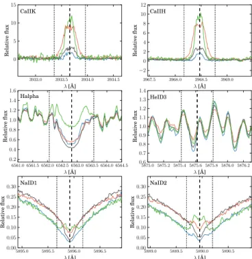
I will now describe in more detail some of the activity proxies which were used in this thesis, namely the Ca ii H & K, H↵, Na i D, He i, and CCF parameters which are the most used optical spectroscopic activity proxies and more easily accessible to the HARPS spectrograph, which was the instrument used to produce the work described in this thesis.
Ca II H and K lines It is known for a long time that the flux on the Ca ii H & K lines has a direct relationship with the number of active regions in the Sun (see e.g. Baliunas & Soon 1995), and therefore these lines are the most used activity proxies nowadays. The use of the double ionised calcium H and K lines as an activity index was made popular among activity researchers by the Mt. Wilson ”HK program”, a project aimed at measuring the long-term activity of solar-like stars which was started in 1966 by O. Wilson (Wilson 1978). Vaughan et al. (1978) introduced the S -index, a dimensionless proxy for the Ca ii activity measured by the Mt. Wilson Observatory spectrometers. This index was based on the flux integrated in 1.09Å passbands centred on the H ( 3933.66) and K ( 3968.47) lines and normalised to the flux in two 20Å wide surrounding
pseudo-continuum bands centred at 3901 (V band) and 4001 (R band)Å. The S -index can be defined as5
S = ↵FH+FK
FB FV, (1.8)
where ↵ is a calibration constant, FHand FK the fluxes in the H and K lines, and FBand FV the fluxes in the two reference lines (e.g. Boisse et al. 2009).
The S -index can be used to control the variations of activity of a given star. However, when the S value of stars of different spectral type is compared, one needs to consider the colour and photospheric contributions to the index. The first arises from the normal-isation of the index to the two pseudo-continuum bands, one bluer and the other redder than the calcium line cores. Stars of different spectral types have different levels of flux on these spectral regions, which will affect the S value. The photospheric contribution is a result of the fact that the H & K line cores are not purely chromospheric in origin, there is also some photospheric flux in the lines. To remove the colour dependence and the photospheric component, Middelkoop (1982) and Noyes et al. (1984) developed a transformation of the S -index into a value R0
HK which is a function of B V and is
normalised to the bolometric flux.
Halpha line As stated before, the most used activity diagnostic are the Ca ii H & K lines which are easily accessible in FGK dwarfs. However, when we move to cooler stars, the energy distribution starts to move to redder wavelengths and the signal-to-noise ratio decreases drastically in the H and K lines. An alternative has been the use of other spectral activity proxies at longer optical wavelengths, and one of the most used is the core of the H↵ line at 6562.808Å (Giampapa & Liebert 1986; Stauffer & Hartmann 1986; Herbst & Layden 1987; Herbst & Miller 1989; Stauffer et al. 1991; Pasquini & Pallavicini 1991; Montes et al. 1995).
Worden & Peterson (1976) noted the central emission line reversal in H↵ lines. While studying 17 dM and dMe stars, Worden et al. (1981) found that this emission is prevalent among the flare (dMe) stars.
5This method, however, is problematic for fast-rotating stars. In rapid rotators, the wings of the H and K
lines fill up the centre of the absorption line and the emission line flux in the core is also lost due to rotational broadening. But in the context of planets searches the fast rotators are normally ignored since, due to the connection between stellar rotation and activity (the faster is the rotation, the higher is the activity), these stars will have a large RV jitter. Nevertheless, Schr¨oder et al. (2009) developed a method to measure Ca ii H & K emission in very rapid rotating stars by comparing the line shapes from known inactive slowly rotating template stars that have been artificially broadened to those of fast rotators.
It has been suggested that the H↵ line may be formed in two distinct layers of the atmosphere: the broad emission component in the low-lying chromosphere and any displaced absorption in the outer parts of the stellar wind (Heidmann & Thomas 1980). Cram & Mullan (1979) studied the behaviour of the Balmer lines (H↵, H , H ). These are weak absorption lines when no chromosphere is present. However, as the amount of chromospheric material (from Te = 5500 K to 50 000 K) increases, these absorption lines first become deeper, then develop emission peaks on the outer edges of their wings, and finally, when the chromosphere is sufficiently massive, they become strong emission lines.
The stellar continuum near H↵ varies along with bolometric luminosity (Hall 1996; Walkow-icz et al. 2004; Cincunegui et al. 2007b) and as a consequence, the flux in the line is expected to vary not only with chromospheric activity but also with spectral type. Therefore, a bolometric correction is needed before the H↵ line can be used to compare the activity of different stars (see Walkowicz et al. 2004).
A positive correlation between the chromospheric fluxes of the Ca ii H & K and H↵ lines has been suggested by several authors (Montes et al. 1995; Strassmeier et al. 1990; Robinson et al. 1990; Giampapa et al. 1989). But the majority of the studies where this relation was observed used averaged fluxes for both lines which were not obtained simultaneously. On the other hand, Thatcher & Robinson (1993) measured the fluxes at a particular moment of each star by using simultaneous observations but they were only observed once. Cincunegui et al. (2007b) measured the long-term variations of the H↵ and Ca ii lines over 7 years for 109 mid-F to mid-M stars and found a wide range of correlations, from strongly positive to strongly negative, to cases with no correlation at all. They found no evidence of dependence of the correlations on spectral type or level of activity. Even when the analysis is restricted to hydrogen line emission stars (dMe), where the conditions on the chromosphere are supposed to produce mechanisms of formation of the lines that are similar, the correlation is different from star to star. The authors also found that the observed correlations are the product of the dependence of each flux on stellar colour and not of similar activity levels. Since both the H↵ and Ca ii H & K lines are generally formed under different conditions, their behaviour can be different when observing different stars with different chromospheric conditions (Soderblom et al. 1993).
Na I D1 and D2 lines The Na i D1and D2resonance lines (D1: 5895.92 Å; D2: 5889.95 Å) can be observed in the spectra of all stellar types, however, for cooler stars
(late-G to M) the doublet starts to develop strong absorption wings. For the most active stars, chromospheric emission in the core of the D lines becomes visible, which is an indication of collision-dominated formation processes. For instance, Worden et al. (1981) observed central emission in the cores of the Na i D lines for dMe stars, and that the emission is strongly correlated with H↵ line emission. The sodium D lines can be used as a complement to the H↵ line for M dwarfs since they provide information of the conditions in the middle-to-lower chromosphere, as opposed to H↵ that is a diagnostic of the conditions of the upper chromosphere and low transition region (Andretta et al. 1997; Short & Doyle 1998; Mauas 2000).
D´ıaz et al. (2007a) studied different features of the D lines using medium-resolution echelle spectra of 84 late F to middle M dwarfs. They defined an index N similar to the Mount Wilson S index: they divided the flux in the core of the D1 and D2 lines by the flux in two redder and bluer pseudo-continuum reference bands. The authors found that when the colour dependence of N and S is taken into account, the correlation between both indices varies from tightly correlated for some stars to cases of no correlation. However, the two indices are well correlated for active stars with emission in the Balmer lines. They conclude that the N index can be useful when comparing the activity variations of individual stars, mainly for later types where little emission is observed in the Ca ii H & K lines. To compare the activity levels on stars of different spectral types, they defined an enhanced index, R0
D (analogous to R0HK for the calcium lines) that takes into account the photospheric contribution to the flux both in the lines and in the continuum windows. As was expected, earlier stellar types do not show any signs of correlation between both indices. However, the R0
Dindex was found to correlate well with R0
HK for the most active stars which exhibit the Balmer lines in emission, even though some of these stars do not present a line reversal at the core of the D lines. Therefore, R0
Dis also a good activity indicator for these stars.
HeI D3 line Another useful diagnostic of chromospheric activity in the optical domain is the He i D3line centred at 5876 Å. This line is normally seen as an absorption feature in F-dwarfs and moderately active G and K-dwarfs (Huenemoerder 1986; Biazzo et al. 2007). The He i absorption requires a temperature of ⇠10 000 K to be formed and therefore, it is a diagnostic of the upper chromosphere, and particularly useful for F-stars in which the other activity indicators in the optical are more difficult to be observed due to the strong continuum flux (e.g. Rachford & Foight 2009)
Parameters of the CCF profile As was stated previously, one widely used and very precise method for the determination of the RV of a star is to measure the wavelength shifts observed in the CCF of the stellar spectrum (for a detailed description see e.g. Baranne et al. 1996; Pepe et al. 2002). The CCF corresponds to an average of all the spectral lines used in the correlation mask (Mayor 1985). As a result, any stellar ”phenomenon” having the ability to influence the lines included in the mask will also influence the CCF line profile (e.g. changing its shape, width, or depth). Asymmetries in the profile of spectral lines can be produced by active regions rotating with the stellar surface (see next section). These effects will be detected in the parameters of the CCF that quantify its profile, such as the line bisector, the full-width-at-half-maximum (FWHM), and contrast (line depth). Consequently, the parameters of the CCF are good proxies of RV induced by activity phenomena. If simultaneous measurements of RV and these parameters are correlated, then it is very probable that the RV variations are being induced by stellar atmospheric changes (e.g. Queloz et al. 2001; Santos et al. 2001; Boisse et al. 2009; Santos et al. 2010).
There are various ways to quantify the shape of the spectral line bisector. The bisector velocity span is the difference in bisector velocity between the upper and lower regions of the line, discarding the core and the wings (Toner & Gray 1988; Hatzes 1996; Queloz et al. 2001). The bisector inverse slope (BIS) is the difference between the mean bi-sector velocity in the 10-40% of the line depth (at the continuum is 0%), and the mean bisector velocity in the 55-90% region of the line (Queloz et al. 2001; Santos et al. 2002). The bisector curvature is the difference between the upper and the lower halves of the line bisector (e.g. Hatzes 1996; Nowak & Niedzielski 2008). For example, an anti-correlation between BIS and RV is often used as a diagnostic of RV induced by spots (Queloz et al. 2001), while positive correlations have been observed for long-term (cycle) observations (e.g. Dumusque et al. 2011a). At these timescales, the FWHM of the CCF profile is also generally correlated with RV while the CCF contrast is normally anti-correlated (e.g. Dumusque et al. 2011a).
1.2.3 Mean activity level of stars
The study of stellar activity is now decades old (e.g. Baliunas et al. 1995; Hall et al. 2007), and the results start to accumulate. In 1957, Wilson & Bappu (1957) detected a positive correlation between the width of the Ca ii K emission and the absolute visual magnitude of stars which is independent of spectral type – the so called Wilson-Bappu effect. This effect can be used to estimate the absolute magnitude of nearby stars by
measuring the Ca ii K width (Wallerstein et al. 1999). Another important result is the distribution of mean activity level. Vaughan & Preston (1980) found that the activity level distribution is not continuous from low activity to hight activity stars, but that there is a gap in the number of moderately active stars. This gap became known as the Vaughan-Preston gap. The majority of the stars with a Solar-like activity cycle appear to have activity levels at around log R0
HK = 4.9 while the rest have higher activity levels near log R0
HK = 4.5, with the gap being at ⇠log R0HK = 4.75 (Henry et al. 1996). However, more recently, early results from the Kepler mission appear to show that the proportion of active stars might be higher than what was expected (Basri et al. 2010).
Stellar activity is also known to have a connection with stellar age. The chromospheric emission in the Ca ii H & K lines and the rotational velocity were shown to be inversely proportional to the square root of the age of the stars – the Skumanich law (Skumanich 1972).
Another important result from the study of the mean activity level of stars is the direct evidence of the dynamo related activity in late-type stars that was shown by Noyes et al. (1984) in the form of a correlation between the Rossby number6andlog R0
HK level. Because of this, the activity level of a star is related to its rotational period (Noyes et al. 1984).
The majority of the activity surveys found in the literature are based on measurements of the Ca II H & K lines. The HK Project at Mount Wilson Observatory operated from 1966 through 2003 and obtained an extensive collection of multiple observations of ⇠1300 stars over a period of 40 years, contributing with a large dataset and long timespan to analyse magnetic cycles in other solar-like stars (Wilson 1978; Duncan et al. 1991; Baliunas et al. 1995). Other large datasets include Henry et al. (1996) (⇠800 stars), Strassmeier et al. (2000) (⇠1000 stars), Wright et al. (2004) (⇠1200 stars), Gray et al. (2006) (⇠1700 stars), Isaacson & Fischer (2010) (⇠2600 main-sequence and giant stars). Lovis et al. (2011) used the HARPS GTO sample to study the relation between magnetic cycles and RV of 304 FGK stars over a timespan of 7 years. More recently, Zhao et al. (2013) published a huge catalog of over 13 000 F, G and K disk stars with measured Ca ii H & K emission. Other large surveys using the H↵ line include that of West et al. (2004) (⇠8000 late-type dwarfs).
Not only is the study of the activity level of stars important per se, but it is also crucial for the field of extrasolar planet research. The activity level of stars is also correlated to the observed RV noise or ”jitter” and can prevent the detection of extrasolar planets
by hiding their RV signal. Strong photospheric features like spots or the inhibition of convection, which are directly related to the activity level of stars, can induce RV noise with amplitudes up to tens of m s 1 (Saar & Donahue 1997; Saar et al. 1998; Santos et al. 2000). Apart from the average activity level of stars which is proportional to their RV jitter, the time evolution of activity is also extremely important for planet hunters. That will be the subject of the following section.
1.3 Stellar activity at di↵erent time scales and its influence
on RV
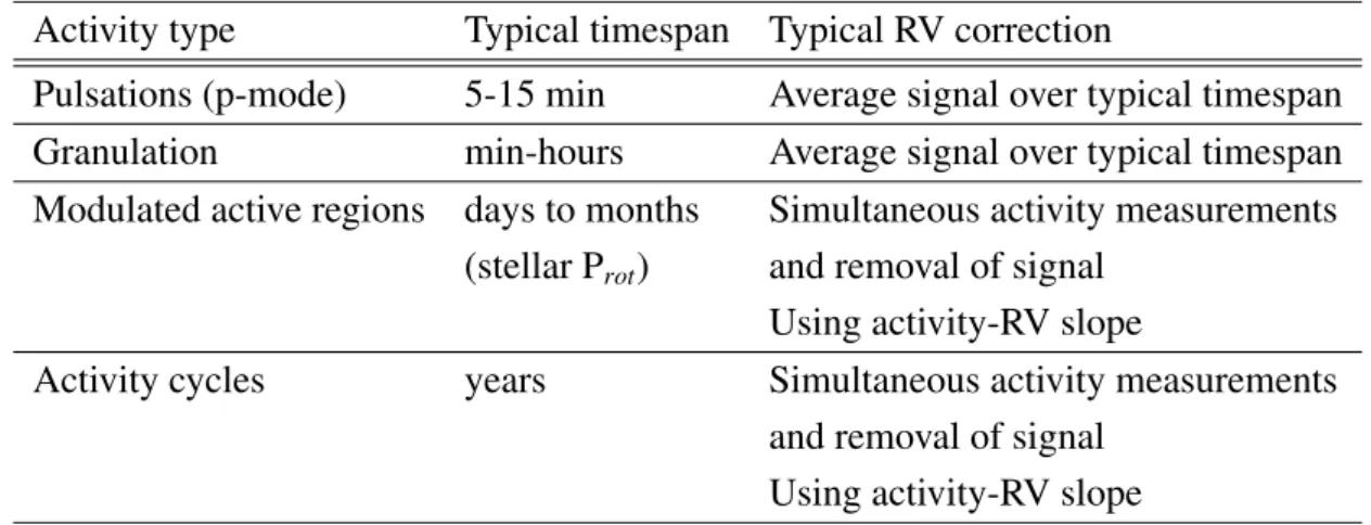
Three distinct stellar intrinsic physical phenomena contribute to perturbations on RV that are considered by exoplanet hunters as ”stellar noise”: oscillations, granulation, and magnetic activity. These physical phenomena have different timescales, or manifest themselves in RV at different timescales. The timescales range from minutes to several years and can add RV noise to potential planetary signals, or even induce periodic signals which can simulate the ones produced by exoplanets. Table 1.1 summarises these types of stellar induced RV noise and gives some examples on how to correct them. In the following sections, we will describe the different types of stellar noise that affect the RV based on their timescales, starting from the short-term effects produced by stellar oscillation modes and granulation phenomena, moving to the effect of rotationally modulated magnetic active regions which affect the RV on timescales similar to the stellar rotation period, and finishing with the long-term effects of magnetic cycles which have periodicities of several years.
1.3.1 Oscillations and Granulation
P-mode oscillations Turbulent convection can excite pressure waves which propagate at the surface of stars with outer convective envelopes and leads to the dilatation and contraction of the stellar external envelopes. These oscillations have timescales of a few minutes in solar-type stars (5–15 min for the Sun; Schrijver & Zwaan 2000) and cause RV variations with amplitudes per mode of up to a few centimeters per second (e.g. Bouchy & Carrier 2001; Kjeldsen et al. 2005). However, the superposition of a large number of these modes can induce RV signals that can reach several meters per second (Schrijver & Zwaan 2000; Bouchy & Carrier 2003; Bedding & Kjeldsen 2003;
Table 1.1: Stellar activity at di↵erent timescales and correction of RV.
Activity type Typical timespan Typical RV correction
Pulsations (p-mode) 5-15 min Average signal over typical timespan
Granulation min-hours Average signal over typical timespan
Modulated active regions days to months Simultaneous activity measurements
(stellar Prot) and removal of signal Using activity-RV slope
Activity cycles years Simultaneous activity measurements
and removal of signal Using activity-RV slope
Bedding et al. 2007). Modern spectrographs such as HARPS, can reach radial-velocity precisions of sub-meter-per-second using short exposure times for bright stars (typically
1 m s 1 in 1 min for a V = 7.5 K dwarf, Pepe et al. 2005). As a consequence, RV
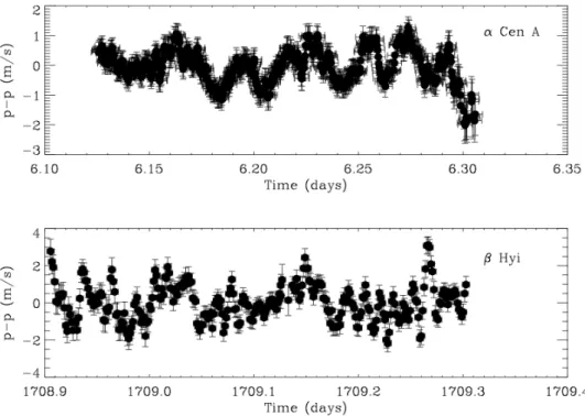
variability produced by p-mode oscillations can be observable and will interfere with the detection of exoplanets (Fig. 1.5).
The frequency of the oscillations scale with the square root of the mean stellar density, while the RV amplitudes scale with the luminosity-to-mass ratio, L/M (Kjeldsen & Bed-ding 1995; O’Toole et al. 2008). As a result, the period of oscillations and amplitude of the produced RV signal will increase towards early-types and evolved stars. This means that F dwarfs will have longer oscillation periods and higher RV amplitudes than K dwarfs and subgiants will have longer period of oscillations and higher RV amplitude than dwarfs.
On the other hand, the lower-mass dwarf stars will be less affected by this type of ”noise” and will, therefore, be easier targets for planet searches. Nevertheless, the noise is still present in these types of stars and can affect the detection of the lower semi-amplitude RV signals induced by planets with low-mass or in longer orbits. It is then necessary to average out this signal in order to increase the RV precision to the sub-meter level. A careful observation strategy, with integer times longer than one or two typical oscillation periods, will be sufficient to decrease the effect of this type of noise below the 1 m s 1 level for dwarf stars (e.g. Santos et al. 2004; Dumusque et al. 2011b).
Tinney et al. (2005) suggested that exposure times of integer multiples of the peak oscillation periods could decrease oscillations induced jitter by 1 to 2 m s 1. Mayor et al. (2003) recommended using exposure times of around 15 min to minimise the impact of
Figure 1.5: RV variations produced by oscillations for ↵ Cen A (upper panel) and Hyi (lower panel). From O’Toole et al. (2008).
oscillations.
Granulation Solar-type stars with an outer convection zone will have a granulation pattern visible at the photosphere. This pattern is made of bright cells, where the hot plasma is rising to the surface, surrounded by darker filaments, where the plasma cooled down and returns to the stellar interior. As a result, these granulation features have positive or negative radial velocity signatures. But, since the brighter granulation patterns are larger than the darker ones, there will be a non-zero average radial ve-locity – the convective blueshift (see Fig. 1.6). This is what produces the ”C”-shapes observed on the line bisectors of solar-type stars (e.g. Dravins et al. 1981). On the Sun, the typical radial velocities of convective motions are 1-2 km s 1. However, the disk-averaged radial velocity jitter will be of the order of the meters per second for the Sun and maybe less for cooler stars (e.g. Palle et al. 1995; Dravins 1990). Granulation has typical timescales up to 25 min (Title et al. 1989; Del Moro 2004). On larger scales in terms of size and lifetime, there is mesogranulation (Palle et al. 1995; Schrijver & Zwaan 2000) and, with timescales that can reach 33h in the Sun (Del Moro 2004), supergranulation, which corresponds to larger convective structures. In active regions, these convective phenomena will be attenuated due to the presence of strong magnetic
Figure 1.6: Illustration of spectral line asymmetries and wavelength shifts caused by granulation. Left: Schematic of the granulation pattern in a solar-type star. Here 75% of the surface is covered by bright outflow granules while the rest is covered by intergranular downflow dark lanes. Centre: Spectral lines representing the bright granules (top profile) and dark lanes (lower profile). Right: The dashed profile is the undisturbed line resulting from a static atmosphere without velocity patterns. The solid profile is the line profile resulting from the combination of the two profiles in the centre panel (average over many granules). The bisector line shows the asymmetry of the profile caused by the granulation pattern. It can also be seen that the core of the line has been blueshifted by this e↵ect. From Dravins et al. (1981).
fields and, consequently, the overall convective blueshift will be lower – there will be an inhibition of convection – and this will affect the measured radial velocity of the star (e.g. Dravins 1982; Livingston 1982; Brandt & Solanki 1990; Gray 1992; Meunier et al. 2010). The effect of granulation on RV has amplitudes similar to those induced by p-mode oscillations, at the meter-per-second level (e.g. Dravins 1999; Schrijver & Zwaan 2000; Kjeldsen et al. 2005; Dumusque et al. 2011b).
The impact of granulation and oscillation modes on RV can be reduced by using careful observational strategies. Dumusque et al. (2011b) arrived at the conclusion that the best observing strategy to attenuate these two effects is to make 3 measurements per night of 10 min each and two hours apart. Using this strategy, they found that a 3 MEarth at the habitable zone (HZ) of a K1 dwarf (with a period of 200 days) can be detectable with HARPS, and therefore, granulation and oscillations will not prevent the detection of Earth-like planets in the HZs of stars. The RV variations induced by granulation and oscillations are dependent on the spectral type and surface gravity of the stars
(Dumusque et al. 2011b). The induced RV amplitude will increase towards early-types and lower gravity stars, implying that an evolved G star will be more affected by this kind of noise than a non-evolved K dwarf.
1.3.2 Rotationally modulated active regions
Active regions are inhomogeneities in the stellar photosphere that are produced by magnetic fields at the surface of solar-type and M-type stars. These features can be dark spots, which have temperatures lower than the surrounding photosphere, and bright plages, which have higher temperatures. In fact, normally active regions consist of both spots and plages.
Since these features have different temperatures than the photosphere, they will affect the spectral lines, by decreasing its flux in the case of spots, or increasing it in the case of plages. As the star rotates, these active regions will move from the blueshifted half of the stellar disk to the redshifted half, attenuating or increasing the flux in the spectral lines as they move, varying the line shapes. This effect will distort the lines and make their centroid, the minimum of the line where RV is measured, move from blueshifted to redshifted, introducing temporal modulations (see Fig. 1.7 for an illustration of this effect). Therefore, an artificial RV signal with timescales similar to that of the rotation period of the star can be produced which will interfere with the signal induced by an orbiting planet by adding noise or simulating false planetary signals (Vaughan et al. 1981; Baliunas et al. 1983; Saar & Donahue 1997; Saar et al. 1998; Santos et al. 2000; Queloz et al. 2001; Henry et al. 2002; Wright 2005; Hu´elamo et al. 2008; Queloz et al. 2009; Lagrange et al. 2010; Boisse et al. 2011). Since spectral lines are distorted due to the presence of spots and plages, one natural diagnostic of activity is the line bisector. An anti-correlation between BIS and RV is normally observed in cases of RV induced by rotating active regions (e.g. Queloz et al. 2001; Hu´elamo et al. 2008; Queloz et al. 2009; Boisse et al. 2011).
For a given spectral type, the properties of active regions depend mainly on their mean activity level, which depends on stellar age. In general, solar-type stars have a tendency to decrease in rotational velocity with time. As they age, their rotational velocities will slow down from around 1-2 days at Myrs to around 20-50 days at 5 Gyrs. As a consequence, the activity produced by the magnetic dynamo will decrease, and active regions will become less proeminent. As a result, younger fast rotating stars will have higher amplitude RV noise. For example, main sequence stars younger than 1 Gyr can
Figure 1.7: Example of a radial-velocity shift induced by a single spot for two contrast values. Three di↵erent phases of the star rotation are shown. Top panel: location of the spot on the stellar disk at di↵erent phases. Centre panel: line profiles (solid) and residuals between the profile of the quiet photosphere and the profile of the spotted star (dashed). Black lines represent a cool spot and red lines a hot spot. Lower panel: observed radial-velocity shift at the di↵erent phases. From Reiners et al. (2010).
have dark spots causing RV variations in excess of 100 m s 1, enough to completely hide a Jupiter-like planet orbiting a Sun-sized star7 To avoid this, young stars are normally not included in planet search surveys. Old, slowly rotating stars are more quiet and, in favourable conditions and a good treatment of activity noise, can enable RV precisions to arrive at the 1 m s 1 level, or even lower (e.g. Queloz et al. 2009; Dumusque et al. 2012). Another approach would be to use near-infrared observations since the contrast of dark spots is expected to be lower than at optical wavelengths (see e.g. Reiners et al. 2010; Hu´elamo et al. 2008).
The effects that spots and plages have on spectral lines could cancel each other if their temperatures were symmetric when compared to the photosphere and their filling factors (the fraction of the disk total area that they cover) the same. However, this is
7Note that for very young stars still in the formation stage, these e↵ects be of the order of km s 1(e.g. Melo