Effective Scheduling of Energy Consumption in Smart Grids

(1)

F

ACULDADE DE

E

NGENHARIA DA

U

NIVERSIDADE DO

P

ORTO

Effective Scheduling of Energy

Consumption in Smart Grids

Jaime Paulo Carneiro Azevedo

Mestrado Integrado em Engenharia Informática e Computação Supervisor: Henrique Lopes Cardoso (Ph.D.)

(2)

(3)

Effective Scheduling of Energy Consumption in Smart

Grids

Jaime Paulo Carneiro Azevedo

Mestrado Integrado em Engenharia Informática e Computação

Approved in oral examination by the committee:

Chair: José Manuel de Magalhães Cruz (Ph.D.)

External Examiner: Álvaro Filipe Peixoto Gomes (Ph.D.) Supervisor: Henrique Daniel de Avelar Lopes Cardoso (Ph.D.)

(4)

(5)

Abstract

This research focuses on demand side management in Smart Grids and the hypothesis of reducing peak demand using Smart Grid capabilities.

Alongside with the production of electricity, concerns related with the efficiency of production, distribution and consumption of produced energy appeared. These concerns arise from the will-ingness of producers to maximize profit and environmental awareness, which is growing everyday in our society.

Driven by that motivation, research in renewable energy resources is increasingly augmenting and potentiating the appearance of new challenges in the production of these cleaner energies, that in addition to be greener are also cheaper in a long term. One of the main challenges is powering all demand with these energies. Renewable energy generators have a long setup time and it proves to be difficult since in peak situations, electricity delivery must be instantaneous, making them dependent on faster delivery time petrol generators to manage peak demands. Managing demand peaks require control of consumer devices which can only be possible nowadays using Smart Gridcapabilities in order to communicate with consuming devices. This approach also demands a certain flexibility of users to postpone or anticipate appliance executions, having as counterpart cheaper energy prices in certain times of the day.

In this research is assumed that electricity prices are known 24 hours in advance, making it possible to schedule home appliances operation. Therefore, using communication abilities of a Smart Grid and electricity prices, this research sets as a main goal to develop an algorithm that can schedule devices in order to help reduce peak demand. This scheduling is constrained by user input, indicating the time frame within which each schedulable device must execute.

The resulting scheduling algorithm is based on a meta-heuristic called Evolutionary Algo-rithms, which uses as a solving technique as a metaphor of human evolution, by trying to mimic crossover between individuals and possible mutations that also happened during human evolution. This method allows to find very good solutions within a reasonable amount of time, making it feasible for a real-world operation. Results are obtained within milliseconds, which for human perception is almost instantaneous.

All goals proposed in this master thesis were successfully completed. Results are promising in terms of employing the proposed algorithm in the production phase of its parent project.

(6)

(7)

Resumo

Esta investigação foca-se no controlo do lado da demanda em Smart Grids e na hipótese de reduzir os picos de demanda de eletricidade utilizado as capacidades de uma Smart Grid.

Com o aparecimento da produção de energia elétrica, surgiram preocupações relacionadas com eficiência energética, distribuição e consumo da energia produzida. Estas preocupações advêm dos objetivos dos produtores de maximizar os seus lucros bem como da preocupação com o meio ambiente, que cresce diariamente na nossa sociedade.

Motivado por esses factos, houve um aumento substancial da investigação na área das energias renováveis o que potenciou novos desafios na produção dessas energias, que para além de serem mais amigas do ambiente, são também mais baratas a longo prazo. Um dos desafios é suprir as necessidades energéticas com essas energias. No entanto, o tempo de arranque dos geradores de energias renováveis é longo, o que torna difícil a utilização destas energias em cenários de picos de demanda energética, pois o fornecimento de energia nessas situações deverá ser instantâneo. Assim, nessas situações são utilizados geradores que utilizam energias fósseis são utilizados.

Gerir os picos de demanda energética requer controlo dos dispositivos que estão do lado dos consumidores. Uma forma de tornar isso possível será utilizando as capacidades de comunicação de uma Smart Grid. Esta abordagem requer também que os consumidores estejam dispostos a adiantar ou atrasar as execuções dos seus eletrodomésticos em troca de preços de eletricidade mais baixos em certas alturas do dia.

Nesta investigação assume-se que os preços da eletricidade são conhecidos 24 horas antes, tor-nando assim possível o escalonamento da execução dos eletrodomésticos. Assim sendo, utilizando as capacidades de comunicação existentes de uma Smart Grid e o conhecimento dos preços de en-ergia à partida, é definido como objetivo para este trabalho desenvolver um algoritmo que faça o escalonamento dos eletrodomésticos com o objetivo de reduzir os picos de demanda de energia. Este escalonamento de eletrodomésticos é feito tendo em conta as preferências do utilizador, lim-itando a execução por uma janela temporal que define o espaço onde a tarefa pode ser executada.

O algoritmo criado é baseado numa meta-heurística chamada Algoritmos Evolucionários, que utilizam uma metáfora da evolução humana e tentam imitar o cruzamento de indivíduos de uma população bem como possíveis mutações nesses mesmos indivíduos. Este método permite en-contrar boas soluções num espaço de tempo razoável, tornando possível em tempo real, enen-contrar ótimas ou muito boas soluções para cada problema numa questão de milissegundos, situação que para a perceção humana é quase instantâneo.

Todos os objetivos propostos nesta Dissertação de Mestrado foram completados com sucesso. Os resultados obtidos são promissores, pelo que é possível a introdução deste algoritmo, para testes, no projeto mãe.

(8)

(9)

Acknowledgements

To my Parents, Jaime e Paula, for all the support during this years at FEUP, for teaching me how to be a good human being and a man.

To Avó Ivone, my first teacher.

To Ana, for all the good times, peace, love and friendship that you give me.

To All my Friends, wherever you are.

To Henrique Lopes Cardoso, for all the patience, support and guidance. You have my deepest admiration and respect.

To David Moura Ribeiro and Fraunhofer for having me at Fraunhofer AICOS, for all the support and work environment.

To Faculdade de Engenharia da Universidade do Porto, for being my second home during my student years.

(10)

(11)

“Listen master, can you answer a question? Is it the fingers, or the brain that you’re teaching a lesson? Oh, can’t tell you how proud I am I’m writing down things that I don’t understand Well, maybe I’ll put my love on ice And teach myself, maybe that’ll be nice, yeah”

(12)

(13)

4.1 Input Data . . . 35 4.1.1 Electricity Price . . . 35 4.1.2 Available Electricity . . . 36 4.1.3 Devices . . . 37 4.2 Schedule Quality . . . 40 4.3 Tests . . . 41 4.3.1 Test 1 . . . 42 4.3.2 Test 2 . . . 44 4.3.3 Test 3 . . . 47 4.3.4 Test 4 . . . 49 4.3.5 Test 5 . . . 51 4.4 Results Analysis . . . 52 5 Conclusions 55 5.1 Future Work . . . 56 References 57

(15)

List of Figures

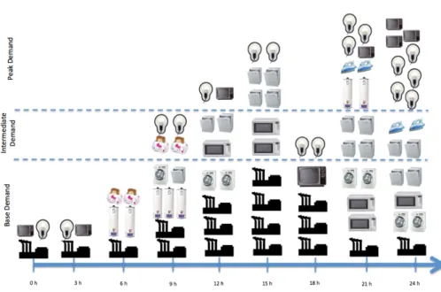
2.1 Peak, Intermediate and Base Demand. . . 6

3.1 Smart Grid, Smart Meter and Smart Devices. (Adapted FromInterconGreen [aI13]) 14 3.2 Task Visual Description. . . 16

3.3 Examples of a Device’s Consumption Curve. . . 16

3.4 Example of a Schedule. . . 17

3.5 Example of a 24 Hour Ahead Pricing. . . 18

3.6 Contracted Power Versus Available Power. . . 19

3.7 Chromosome Representation. . . 22

3.8 Gene Representation. . . 22

3.9 Time Frames Choice. . . 24

3.10 Roulette Wheel Selection. . . 27

3.11 Start Time Probabilistic Choice Within Possible Domain. . . 27

3.12 Architecture of the Main Project. . . 32

3.13 Architecture of the Scheduler. . . 33

4.1 Pricing Curve . . . 36

4.2 Electricity Curve . . . 37

4.3 Dish Washer Consumption Curve . . . 38

4.4 Washing Machine Consumption Curve. . . 39

4.5 Drying Machine Consumption Curve and Task’s Preemptive Division. . . 39

4.6 Algorithm’s Output . . . 43

4.7 Available Power and Consumed Electricity by Test 1 Schedule . . . 43

4.8 Results Within 4 Seconds Time Limit. . . 45

4.9 Optimal Consumption Curve. . . 46

4.10 Near Optimal Consumption Curve. . . 47

4.11 Optimal Scheduling Found. . . 48

4.12 Optimal Consumption Curve. . . 49

(16)

(17)

Chapter 1

Introduction

This research focuses on demand side management in Smart Grids and the hypothesis of reducing peak demand using smart grid capabilities. The necessity of reducing peak demand in order to increase base demand powered by renewable energy sources is one of the main challenges in the electricity industry for the twenty-first century. This research tries to contribute on solving this current problem by aiming at optimizing customer’s electricity usage. Scheduling and shifting electricity usage to more advantageous time frames within customer’s flexibility and will to help producers. Typically, customers are rewarded with some kind of advantages in order to make up for their flexibility in electricity usage.

After this initial introduction to the problem, in the following section we explain the motivation towards for this research, enumerate the proposed objectives, and point out some obstacles for this work. In the end of the chapter we explain the structure of this document.

1.1 Motivation

Alongside with the production of electricity, concerns related with the efficiency of production, distribution and consumption of energy appeared. These concerns arise from the willingness of producers to maximize profit and environmental awareness, which is growing everyday in our society. These concerns do not only come from producers, but also from governments that are in-creasingly regulating and legislating energetic sectors. Furthermore there is a growing investment and financing in research sustainable energy [All13a, Sys13, Wee13], specially in the European Union, providing for Intelligent Energy research 730 MillionAC available from 2007-2013 [Eur13]. When this subject firstly appeared, the initial focus was on production using fossil energy re-sources. Production took place in central stations that fueled an unidirectional distribution system, which is used even today. In order to minimize losses in this type of systems, research on possible optimizations in the process of electricity generation have been conducted. These researches made possible the increase of produced energy for the same amount of energetic resource [CKW+12].

Although these optimizations have improved existing systems, greenhouse gas emissions are still increasing due to the growing consumers’ demand of energy from year to year. For this

(18)

Introduction

reason, research for greener energy resources has emerged, from natural gas, hydro, wave and tidal, wind or even solar energy. Many were the energy resources studied for producing energy in order to reduce greenhouse gas emissions. This research has shown that solar and wind energy were the easiest, greenest and production from these sources result in a very low environmental impact [CKW+12, CKV11, LSS12].

Despite being cleaner energies, their generation depends on a very specific technology and variable natural factors that make these resources difficult to integrate with the network [ZW11]. This way, these energy resources are less usable unless they can take a significant part of base production. In order to be able to take advantage of this, base demand must be constant, meaning that peak demand must be reduced.

With the appearance of this problem, energy producers began introducing plans for energy con-sumption where prices depend on energy demand, in order to reduce peak concon-sumption [HG10].

It has quickly become apparent that, even with these measures, there is a need to transform the existing power grid into a “smarter” grid that could offer flexibility, allowing better possibilities of solving the problem. Thus, the appearance of Smart Grids started a new path in finding solutions for this problem by enabling exchange of information between the producer and the consumer in order to control and advise consumers about their energy usage[Kri10].

Consumption control brings advantages by serving as a top aide in deviation of consumption to non-peak hours, thus enabling a constant production, bypassing the difficulties in production of wind and solar power [CKW+12, CKV11, EMCA+11]. This research will be focused on po-tentiating this consumption control advantages with the utilization of a device, which is present on the Smart Grid: the Smart Meter. With this technology, consumer appliances’ power demand can be controlled and monitored individually making the energy consumption schedulable. Thus, all consumers will become able to help solving the peak demand, which is the main focus of this work.

Knowing the factors involved in this type of problem, objectives in order to control peak de-mand must be defined to serve as guidelines during this research. In the next section we explain these guidelines.

1.2 Objectives

To pursuit the solution of the aforementioned identified problem, this section points out the goals proposed for this research. Knowing the motivation of studying this type of problems, shown in section 1.1, the main goal is to reduce demand peak in a Smart Grid by controlling consumer’s energy use. The hypothesis in this research is:

• Is it possible to create a system that schedules and controls power consumption of household devices, in order to align energy demand with energy production, reducing peak demand?

(19)

Introduction

In order to help finding answers for the hypothesis proposed some specific goals are pointed out:

• To study the best approaches existent in energy scheduling problems identifying the best practices in energy usage;

• To study devices belonging to consumer’s side in Smart Grid’s architecture such as Smart Metersand their capabilities;

• To study existent palette of algorithms that schedule power usage in the demand side in order to understand pros and cons of each one;

• To identify the most relevant factors that can influence the scheduling of consumer’s devices; • To develop a software prototype that controls demand on consumer’s side and will be

run-ning on a low processing power machine called Smart Meter.

This work will be part of an National research prototype called EnAware that is being built currently and has another features such as low level communication between appliances and a Smart Meter, enabling the software prototype decisions to be put into practice.

Knowing the main goals of this research, the structure of this document and its content is explained in next section.

1.3 Main Contributions

These are the main contributions from this work.

• Realism of the addressed scenario.

This contribution allows scheduling to be more realistic and reduce error when estimat-ing the consumption curve of each computed schedule by givestimat-ing full emphasis on devices’ consumption precision. Also introduce preemptive appliances. With this new perspective on appliances’ execution it will be possible postpone some of its parts in order to manage energy consumption or to take advantage of floating prices. Finally introducing a time pre-cision of 1 minute bringing more time accuracy when scheduling. With this, fine tuning each schedule is possible, enabling even more precision in energy consumption.

With this, less energy waste is generated, providing a greener scenario, which is an objective on this type of problems.

• Algorithm performance that permits real-time usage.

Researched algorithm’s performance delivers instantaneous and optimal or near optimal solutions, which is a very good progress in this area.

(20)

Introduction

• Testing in real life.

The proposed solution will also be tested in a live test case that will, in the future, testify the advantages of this new approach on reducing peak demand.

1.4 Research Context

This research is part of a national research project hosted by Fraunhofer AICOS named EnAware. EnAware is a project that proposes to electricity consumers a new way of looking to their energy consumption in order to save money and protect the environment. This project contains a vast selection of tools that enable, by using a Smart Grid, consumers to control remotely energetic consumption by introducing some usage preferences that enable money savings. This is the mod-ule where this dissertation is deeply connected: scheduling appliances in order to reduce peak demand for producers and help customers to save money.

1.5 Document Structure

Besides this first introductory chapter, this document has five more chapters. In Chapter 2 a Litera-ture Review to some relevant and different approaches on this problem is made. These approaches are discussed and pros and cons of each approach are presented.

In Chapter 3 the working scenario is explained in order to contextualize the reader about the different types of tasks. Details about the meta-heuristic used to help solve the problem are also provided, alongside with the motives that ground the decision. Finally, the architecture of the scheduler is explained in full detail.

In Chapter 4 extensive tests are made with a vast palette of scenarios, followed by the results and respective analysis of results. Different type of evaluations, both qualitative and quantitative are made as well as discussion of results.

In the last chapter, Chapter 5, conclusions of this research are presented as well as considera-tions about future work.

(21)

Chapter 2

Literature Review

This chapter studies previous approaches to peak demand control problems, by identifying their context and challenges. Firstly the Smart Grid concept is introduced, together with its components, as well as its capabilities and potentialities. It is also shown why this innovative grid is the perfect framework for this problem.

Since the beginning of electricity production, one of the main challenges relates to predict how many energy is necessary at each moment in order to fulfill the needs of consumers at any time. Many researches were performed in order to predict with the most certainty how much energy will be needed from customers in order to avoid energy waste. These predictions are difficult to perform since a considerable amount of energy consumed is coming from random actions performed by users. However some electricity usage is related to the human activities, such as during mealtime or night entertainment, which intervals can be determined previously in order to fulfill that demand. In order to categorize electricity consumption, producers created a nomenclature for the amount of energy needed by customers. Figure 2.1 shows a graph that divides the consumption during day into 3 categories: base demand, intermediate demand and peak demand.

Base demand relates to the minimum energy that must be produced in order to fulfill minimum demand from customers, typically during nighttime. Intermediate demand is normally reached during daytime when the industry’s is consuming energy. Peak demand are events that occur when energy demand is substantially higher than expected, making this type of demand a very problem-atic event to solve. Peak demand normally forces producers to turn on auxiliary energy generators that typically use fossil energies in order to run. These events are very costly to producers because of the rising prices of fossil energy fuels, which also are very harmful for the environment. What if producers could control these peak demand intervals? What if was possible to exchange this fossil energies to environmentally friendly energy sources? These possibilities would also bring economical advantages for producers, since renewable energies’ production costs are cheaper.

In order to include renewable energy sources, peak demand must be reduced. Renewable ener-gies’ generators do not have the same response time as fossil fueled generators, since they depend on natural factors such as wind or sunlight, therefore they cannot be a solution in emergency

(22)

sit-Literature Review

Figure 2.1: Peak, Intermediate and Base Demand.

uations. The solution involves shifting peak consumption to non peak hours, enabling the base demand to be higher and therefore use this renewable energy sources. In order to address this problem, a subject was created in order to study ways of controlling demand named Demand Side Management.

Demand Side Managementis heavily desired since it brings control in the consumer’s side of the grid [Kri10, HG10]. One of the first methods used in electricity industry to reduce demand peaks was Demand Management by Contract[HG10]. This contract sets different fixed contracted prices for the energy. Typically this contract imposes 2 or 3 different time intervals, which have dif-ferent pricing according to producer’s expectations [dP13]. The price is higher when the chances of having a peak in demand are higher. With this, electricity companies expected customers to use non-priority appliances in cheapest shifts. Despite being very rudimentary, this method is used nowadays in Portugal [dP13].

This type of demand management has serious drawbacks. Household appliances used nowa-days are mainly manual, making them dependent of a human being to operate them. So, this method is very dependent on practicability and willingness to control devices and, consequently, save money on electricity. Thus the non practicability of this method, makes the system unpre-dictable and dependent [HG10].

The appearance of Smart Grids brought a new hope on this subject, bringing automation and planning to consumer’s electricity usage. With this, peak demand during all day can be controlled and reduced by applying specific methods such as scheduling, which will be explained later in the document.

(23)

Literature Review

2.1 Smart Grid

Smart Gridis a two-way electricity transmission infrastructure that possesses the ability not only of transmitting energy but also information between consumers and producers. The idea behind this type of system is to transform the current one-way power grid into a more collaborative system that enrolls not only producers but also consumers, making energy production and distribution more efficient, reliable and sustainable [Com08].

This improved grid brings a new paradigm for reliability. This paradigm includes a fault de-tection and self-healing systems that ensure minimum hassle in returning to normal energy supply. With these features, the network can predict power shortage and reroute the power needed. It also can solve energy distribution problems automatically with many techniques such as distributed multi-agent systems [STYP10, Com08].

Bidirectional energy flow is another characteristic of the Smart Grid system. It allows energy supply to be not only from the main producer but also from consumers. Consumers have the possibility of connecting their own power supply systems, such as photo-voltaic panels or energy store cells [EMCA+11]. This enables the energy company to buy from customers and avoid turning on emergency generators that typically are fossil-energy fueled.

This flexibility featured on this new grid enables the consumer to be an energy seller and so reward the effort and investment made in energetic generation and storage systems. On the other hand, the ability to transmit energy prices helps consumers decide if they are willing to pay the price of electricity on that time or postpone the usage of electricity to when it is cheaper [Com08]. Efficiency and sustainability is brought by the grid’s ability to predict and regulate energy demand. With this knowledge production of energy using “greener” sources, such as solar or wind, can be more accurate. Thus production and distribution become more efficient using only the needed energy, evading the loss of unneeded production and increasing in sustainability due to power sources’ nature [CKW+12, Com08].

Efficiency brought by this new grid requires a consumer’s side equipment which manages appliances and their working times. This equipment, called Smart Meter makes all the communi-cation between consumers and grid.

2.1.1 Smart Meters

The Smart Meter is a powerful and indispensable tool for a Smart Grid [DD08]. Along time electric meters evolved from a simple electricity reader to a capable machine that has some pro-cessing power. These devices are now designed to be capable of using network connections with other devices in order to communicate with suppliers or smart devices that are using energy. Also Automatic Meter Reading(or AMR) enables a whole new range of possibilities in managing the electricity usage in the consumer’s side since it can read in real-time energy consumption [Kri10]. With these capabilities the Smart Meter is able to control the energy load of all smart equip-ment connected to it. Each smart device connected to the Smart Meter has a programmed thresh-old. This threshold represents the maximum energy that can be required by each smart device.

(24)

Literature Review

When this threshold is reached the Smart Meter disconnects the load using its communication capabilities.

Smart Metersalso allow the user to control remotely the devices, turning them off and on if necessary. Besides that it allows the producer to communicate the prices, the needs of reducing power usage and other information that need to be known by the Smart Meter. These capabil-ities enable the producer to block consumers’ access to electricity due to non-payment almost instantaneously [BZ13].

Distributed electricity generation became possible with this equipment, it may be used to man-age when to use the produced energy and when to sell it [Kri10]. This manman-agement is possible due to Smart Meter’s processing capabilities.

Compiling all these features, the combination of communication and processing capabilities brings us to the key point in peak control, making Smart Meters the key to manage consumer’s side need for electricity. This device also brings the possibility to include specific algorithms that schedule power usage taking into account the user’s preferences, postponing usage of non-priority equipments to non-peak hours. This device helps producers to make a more efficient and reliable distribution policy. Another direct consequence is the savings in electricity by the user because typically the off-peak electricity price is lower [Kri10].

2.1.2 Smart Devices

Demand Side Management in Smart Grids implies that all schedulable equipment connected to the Smart Grid is able to communicate and receive orders from a Smart Meter, which runs the scheduling algorithms. With Smart Devices, the system can run without human intervention.

Another key feature of Smart Devices is related to the priority of each device on using elec-tricity. This means that some devices can be scheduled, such as washing machines, water heaters or dishwasher machines if the energy is not available or it is not convenient to use it at that time.

Next subsections explain the most relevant approaches studied using these devices in order to schedule their power usage helping reduce peak demand.

2.2 Related Work

After this initial introduction with examples prior to the appearance of Smart Grids, literature review reveals some relevant research in Smart Grid demand side management. In this section we address to some relevant approaches similar to our hypothesis in order to understand what were the conclusions and the progress achieved in this area.

(25)

Literature Review

2.2.1 Active Demand Side Management Using Photovoltaic Panels and Neural Net-works

Matallanas et al. [EMCA+11] propose an implementation of a active demand side management based on Artificial Neural Networks. The studied system features photovoltaic panels as gen-erators and the scheduling is made to optimize the usage of the generated energy when its pro-duction is at peak. So, these neural networks are implemented with the objective of maximizing self-consumption of each individual device connected to the Smart Meter. In other words, this scheduler tries to maximize the usage of panel’s production in real time since there do not exist storage devices to keep the generated energy.

Concerning to user preferences, this system allows the user to choose time frames when de-vices can operate; for instance the dish washer may operate from 1 pm to 8 pm. Knowing this, the system predicts photovoltaic generation for the next day and with all this makes the scheduling plan for the equipment to run.

Although this system utilizes a smart meter, it does not communicate with the energy supplier or other producers.

2.2.2 On-line and Off-line Scheduling Minimizing Electricity Average Cost

In [KT11] the problem is addressed in two different off-line modules. The first module is a sched-uler that calculates preemptive tasks with a load balancing algorithm that implements a Valley Fill-ingmethod. Non-preemptive tasks are served as a Bin-Packing problem, in other words, the tasks are served as long as there is enough energy to feed the equipment. In this approach the authors use user time and task preferences, task duration and power requirement as objective functions for the scheduler.

Also in [KT11] two on-line demand schedulers are studied. In the first dynamic approach the algorithm simply chooses if a preemptive-type task is served as it arrives or is served at deadline minus the time of the task. The second method named by the authors as Control Release has a threshold limit. If the electric usage is below a given threshold the task is performed, if not the task is queued. If electricity usage is not below the threshold until the deadline of the task, the task is performed anyway.

There is a delaying factor that worsens as long as the task is postponed, making the task more likely to be chosen next due to scheduler’s preferences.

These four methods (two on-line and two off-line) consider minimizing the longterm average cost. The values used for taking decisions are only related to electricity usage.

2.2.3 Scheduling Using a Desired Load Curve as an Objective

In [LSS12] the authors propose a day-ahead scheduler that uses load shifting as a primary load management method. The objective function is not fixed and system requires a load curve as the model for electricity usage. Also, with the injection of these curves to the system, the

(26)

Literature Review

primary objectives of the energy consumption can diverge, from price reduction to peak reduction, depending on user’s preferences.

The used algorithm is a Genetic Algorithm that takes the load curve as an objective curve and tries to achieve the similarity between the real curve and the input curve.

During the scheduled day on-line actions are scheduled based on the actual state of the system.

2.2.4 Real Rime Pricing Using Stackelberg Game Model

In [CKV11] the authors propose a smart real time pricing (RTP) scheduling using a Stackelberg game model. This model implies that consumers and producers play a role between two possible: follower and leader. In this model, followers answer only after and regarding leader’s action.

In this approach the producer leads by setting electricity’s price and consumers, Smart Meters use electricity pricing to take action. This approach takes into consideration a special type of preemptive smart devices whose consumption can vary during time to help the overall power consumption. As they refer, there are few examples on this type of devices, for example, electric car batteries.

The method uses the Smart Meter as a controller / scheduler and tries to minimize each in-dividual appliance usage cost. The scheduler chooses within the time-frame chosen by user, the best time to run each device. Delaying the task from its start implies an inconvenience cost that is taken into consideration in scheduling.

Pricing is defined by the provider as a vector that contains prices for a specific amount of time. Regarding this vector the scheduler calculates the best starting time for each Smart Device connected.

Authors refer that this approach stands above day-ahead pricing because it avoids the similarity demand between users which can provoke peaks by the rising electricity demand. Also it relies on real pricing and not in predictions like in day-ahead pricing.

2.3 Summary

All these approaches have shown various ways of controlling users’ electricity usage. However there are issues related to this methods. One of these issues is related to communications between producers and consumers: some of the approaches fail to communicate with some time ahead in order to prepare the system to make decisions ahead of time, enabling the system to have more probability of succeeding on scheduling tasks.

Approach [CKV11] has that issue and approach [EMCA+11] does not communicate at all. Another issue is related to the type and scheme of input. Approach [LSS12] is an example of a less intuitive input. It uses a load curve to inform the scheduler how the user wants the load curve to be like.

Finally in approach [KT11] and [CKV11] start their method by trying to make approximations of how the grid will behave, leaving a very small room for finding an optimal solution.

(27)

Literature Review

For all these reasons this research has proposed a very different approach to this type of prob-lems. The proposed approach is explained in full detail in the next chapter.

(28)

(29)

Chapter 3

Effective Scheduling in Smart Grids

This chapter will address the work performed during this research. Firstly we explain the sce-nario and some concepts that are deeply connected to this research. The different task types are explained in order to understand how each one affects scheduling procedures and the final results. Alongside with each type we show adjacent information about each task type.

After these introductory concepts, we explain how a schedule is composed as well as electric-ity pricing and available electricelectric-ity concepts, emphasizing how they are deeply connected to the finding of a good schedule.

Next the developed approach, based on the genetic algorithms meta-heuristic, is explained, including the rationale behind this choice. We also show the architecture of the developed system.

3.1 Scenario

This research aims to help control household devices, but since each house has it’s unique config-uration, some notions about this project must be defined in order to understand the prerequisites necessary to enable scheduling and how is scheduling possible with all these possible combina-tions of household appliances. In this section we present the scenario for this problem as well as some notions which are important to fully understand the subsequent sections.

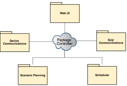
As Figure 3.1 shows, each household must have access to the Smart Grid. Also each house must have an appliances controller and energy meter called Smart Meter and some Smart Devices which are appliances that can be controlled over the Smart Grid, see 2.1.

Each device is connected to the Smart Meter that controls and manages electricity requests. With this configuration it is possible to control each device remotely and automatically making not only electricity transmission but also gathering live information about the devices.

Typically, when users need a household appliance to execute a determinate job, they turn on each device at desired start time so they can finish near desired hour in order to help users to fulfill their needs. Undoubtedly, nowadays, with people living an increasingly busy life, the simple action of turning on a washing machine or a dish washer can become very inconvenient. Aside this fact, with the appearance of Smart Grids and floating prices, scheduling household devices

(30)

Effective Scheduling in Smart Grids

Figure 3.1: Smart Grid, Smart Meter and Smart Devices. (Adapted FromInterconGreen [aI13])

became a necessity. With this new paradigm consumers can shift each device start time in order to take advantage of cheaper energy. So, what if users can choose, ahead on time, the end time of each household device execution? With this possibility, users can pre-schedule appliances when it is more convenient. In practice, it will be possible to perform instructions to the system such as:

“I want my washing machine to run between 7pm and 8am, the oven to be cooking for 45 minutes and be ready at 9pm and the dish washer to end before 8:45pm.”

With this newer approach to household duties, some challenges appear, such as knowing each device’s execution time for each program offered or even how to define an execution timewise.

Scheduling household devices efficiently in order to reduce electricity peak demand is a key point to explore in this work. For the purpose of this work, these devices can be referenced as tasks, since each one of their operations represents a task with a deadline and execution time for each individual program they run. It is important to mention that not every household device can be scheduled. Knowing this, some considerations and definitions about the different types of tasks must be explained.

3.1.1 Tasks

Naturally there are tasks that must be running as soon as they are triggered, otherwise the user’s experience may be harmed. These tasks are categorized as non-schedulable since they cannot be postponed or delayed fully or partially. Some examples are: lights, using a hairdryer or watching TV.

(31)

Despite the non-schedulability of the tasks, they can provide valuable information to the sys-tem such as their consumption curve, execution time or even periodicity. This information can be used to make a track of how much energy is likely to be available when scheduling other tasks, as we can see in 3.1.4.

On the other hand, schedulable tasks are more flexible. These tasks can be delayed within user’s preferences, enabling the system to choose the best start time for each task regarding the actual price of electricity as well as the usage of electricity at any given time. This scheduling ability help consumers by reducing electricity bill and keep track if the contracted power is truly needed, as well as helping producers and saving the environment by reducing peak demand.

3.1.1.1 Preemptive vs Non-Preemptive Tasks

These types of tasks are schedulable tasks. But they also can be divided into two different groups: • Non-preemptive tasks - This task type allows scheduling but the task cannot be divided.

This means that when a task starts it cannot be stopped until full completion.

• Preemptive tasks - In addiction to be schedulable, this task can also can be divided into sev-eral (sub) tasks for more flexibility in scheduling. The division must be defined previously according to machine’s internal events. Despite the fact that these tasks can be divided, each sub-task must run after the previous one end.

This research contemplates the two types of schedulable tasks described above. As these two types of tasks can be scheduled, some informations must be known about each task. The information regarding one schedulable non-preemptive task is the following:

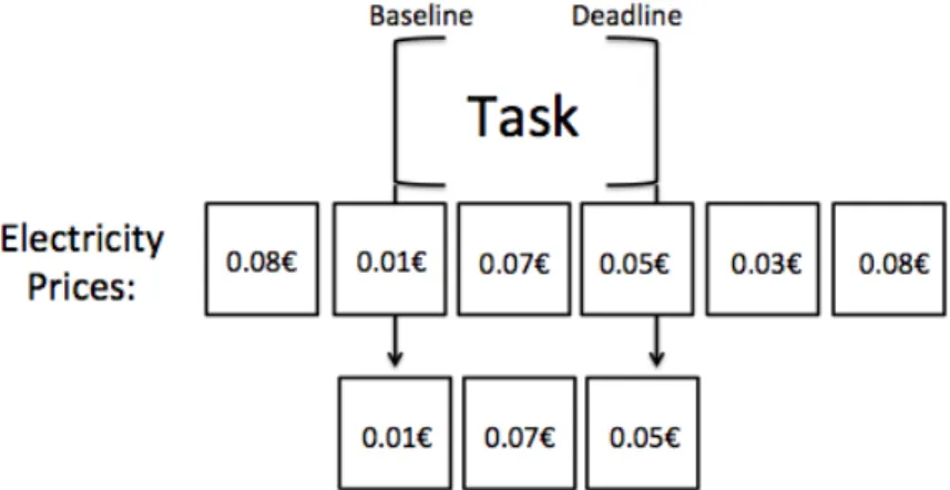
• Baseline - Earliest possible start of the task; • Deadline - Latest possible end of the task; • Duration - Duration of the task in minutes;

• Start Time - Calculated task start time for the best overall schedule found;

• Consumption(t) - Consumption of the task in watts, at execution time t, see 3.1.1.2.

Figure 3.2 shows a visual representation of the task and how consumption curve is seen during execution. To represent a preemptive task, there is a need of defining the set of tasks that are parts of the main task. To maintain their sequencing, each task has a reference to its predecessor. This information must be known for each tasks and it is used to prevent malfunctioning of devices. In its most atomic form, preemptive tasks are indeed non-preemptive tasks since their division repre-sents their divided internal working cycles.

(32)

Figure 3.2: Task Visual Description.

3.1.1.2 Task Consumption

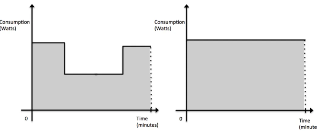
In addition to task’s timing information, there is one special item that composes a task called consumption curve. Each task has a consumption curve associated. This curve represents the electricity usage during the task’s execution time. For each program that can be executed on each device, the scheduler must have the information about its consumption in order to enable an accurate schedule’s total energy consumption maximizing the authenticity of the schedule. Figure 3.3 shows two possible examples of a consumption curve for a task.

Figure 3.3: Examples of a Device’s Consumption Curve.

There are some devices that possibly can have this variable consumption curves such as dish washers or washing machines that during some intervals of their executions use more energy, for example, when heating water or less energy, when flushing the water out of the machine. Other devices such as microwaves have a constant consumption curve, meaning that the consumption in every moment of the execution is the same. After this definition of all schedulable tasks, the next

(33)

subsection shows how these tasks can be combined and defines some characteristics of a set of tasks.

3.1.2 Schedule

A schedule is a set of tasks that are combined in order to meet user’s preferences for all devices. For the purpose of this work, a schedule is valid if it fulfills the following criteria:

• The schedule contains all schedulable tasks within a time frame of 24 hours; • All tasks must be executed and terminated within its baseline and deadline;

• No part of a preemptive task can have its start time before end time of its previous part; • Energy consumption cannot be above the available power at each moment.

Atomic time unit is 1 minute, meaning that schedule precision is within 1 minute time.

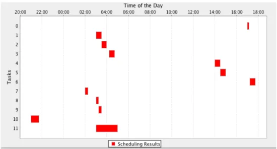
Figure 3.4: Example of a Schedule.

In figure 3.4 we can see a possible schedule for one day. One valid schedule is better than another if its total cost is below the other’s cost, meaning that the lowest cost, the better schedule. In order to know the cost of each schedule there must be the information about electricity prices at each point in time. Also, electricity prices are used to calculate the start time for each task. This issue is addressed in the next subsection.

3.1.3 Electricity Price

One of the main features of a Smart Grid is the ability to communicate data in addition to power transmission between producers and consumers. This data connection makes possible real time

(34)

information between all terminals connected to the grid. One of such informations is price of energy.

Literature review [KT11, CKV11] has shown that transmission of energy prices can be per-formed in various ways, being the two more relevant the 24-hour-ahead pricing and real time pricing. In this research 24 hour ahead pricing was chosen as a main pricing announcement pol-icy, because it enables the scheduling system to have a decent time window to schedule the tasks and plan the best schedule. This makes scheduling easier and with better results since sched-uler knows beforehand what are the prices and when they will be in place, making it possible to maximize profit. On the contrary, real time pricing would lead to unexpected price changes and consequently less flexibility to better adapt the schedule to changed prices since not every running task can be stopped.

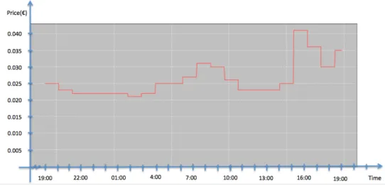
Another key information pricing gives is that, pricing for the next 24 hours resembles produc-ers’ intention on where to reduce electricity demand [RW08]. To achieve that, producers increase the price of kW/hour on some time frames and decreases in other ones in order to reward cus-tomers that have flexibility to change their demand from peak to non-peak hours. In this research the price of energy is the key factor to perform scheduling since it is the only factor on the whole Smart Gridsystem that informs customers on producers’ intent of reducing or increasing electric-ity consumption.

Figure 3.5: Example of a 24 Hour Ahead Pricing.

Figure 3.5 shows one possible pricing curve for the next day’s scheduling.

3.1.4 Energy

Another essential piece of information for scheduling concerns the but also availability of energy. Electricity supply is limited. Each household typically has a contracted power limit. Contracted

(35)

power is the maximum electric energy available for a specific customer. Typically producers pro-vide several contracted power limits so customers can choose the one that better suits up more to their necessities. When the contracted power limit is exceeded, energy supply is automatically interrupted, shutting down all electric devices. This contracted power must cover both schedulable and non-schedulable tasks. This makes more difficult to predict how much power will be available since non-schedulable tasks are more difficult to predict. Sharing the power with non-schedulable tasks also narrows the range of possible solutions and can make scheduling more difficult.

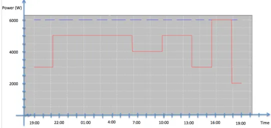
Figure 3.6: Contracted Power Versus Available Power.

Figure 3.6 shows an example the correlation between contracted and available power. The slashed line shows the contracted power between customer and producer and the continuous line represents the available power for running schedulable tasks. There is no way of predicting with 100% confidence the energy that will be used by customers on non-schedulable tasks. This con-sumption depends on human behavior that can be very random. Other factors that enable more random results include temperature, because it affects the way the climatic devices are used, or sunlight, that affects artificial light usage. There are many possible approaches to deal with this problem such as forecasting algorithms, data mining or machine learning [MM09, TdMM06].

Since prediction non-schedulable energy consumption is not the main purpose of this research, we will assume that available power is given as input for the scheduler. This input can be calculated as an average of previous 72 hours non-schedulable devices’ consumption or another method that suits this purpose.

In each minute of the day, available power is contracted power minus the average of used power on non-schedulable tasks.

After revising all factors that compose or can influence a schedule, we now turn to explaining the scheduling algorithm proposed, including the meta-heuristic adopted.

(36)

3.2 Scheduling Algorithm

This section contains all the information related to the scheduler created, including detailed in-formation of each one of its components. Literature review has identified, besides different ap-proaches to this type of problems, some algorithms that could be used as a starting point to this problem. In in this research was chosen to create a task scheduler using Evolutionary Algorithms. Evolutionary Algorithms are meta-heuristics that try to mimic the biological evolution of species. Inheritance, crossover, mutation and selection are the key techniques that are compu-tationally replicated in order to reach near optimal solutions.

In this research, there are some reasons why evolutionary algorithms were chosen. One of the shortcomings of this type of algorithms is that there is no guarantee for optimality. In this particular case, an optimal solution is not required since the quality of each solution is related to billing of energy. Being a soft constraint, price is not in critical matters such as task precedences or exceeding the available power, which are the hard constraints in this problem. Also, there are many possible solutions in each task that despite not being optimal bring noticeable reductions in the final price of each schedule.

Another reason for choosing evolutionary algorithms is the fact that the search space is very large and complex, due to the power, price, precedence constraints and time granularity being 1 minute. For instance, considering a schedule for 3 simple, non-preemptive tasks their number of possible start times is presented in Table 3.1.

Baseline Deadline Duration Number of possible start times Task 1 0 min 60 min 10 min (60 - 0) - 10 = 50 Task 2 0 min 120 min 60 min (120 - 0) - 60 = 60 Task 3 0 min 45 min 5 min (45 - 0) - 5 = 40

Table 3.1: Number of Possible Start Times for a Simple 3 Task Schedule.

If the three tasks shown in Table 3.1 are to be combined into the same schedule, they could generate 60000 different start times for the search space, turning a small sized problem into a relatively big domain.

Being a stochastic and parallel meta-heuristic, an evolutionary algorithm helps the system not to stuck on local-optima solutions and enables the possibility of finding good solutions very quickly. Another reason for selecting evolutionary algorithms is related to the vast array of re-searchers on scheduling problems that have successfully used this approach.

3.2.1 Evolutionary Algorithms

As previously mentioned Evolutionary Algorithms emulate biological behavior in order to reach the best solution possible for each problem to be solved. Typically, an evolutionary algorithm is composed of a population of chromosomes characterized by genes. A fitness function is used to evaluate each chromosome, which are combined through a crossover function and altered using a mutation method. Figure 1 shows the algorithm that explains one execution of an Evolutionary

(37)

Algorithm.

Algorithm 1 Evolutionary Algorithm

1: GeneratePopulation(NIndividuals)

2: while (BestIndividual.Fitness < MinimumFitnessRequired) do

3: for all (Individual in Population) do 4: CalculateIndividualFitness 5: end for 6: ChosenIndividuals← Choose2Individuals() 7: NewIndividuals← Crossover(ChosenIndividuals) 8: if (ProbabilityOfMutation()) then 9: Mutate(NewIndividuals) 10: end if 11: ReintroduceIndividualsIn(NewIndividuals, Population) 12: BestIndividual← MaxFitnessIndividual(Population) 13: end while 14: return BestIndividual

Initially the algorithm starts by generating a population of N individuals as chromosomes, that will be the first set of elements analyzed and evolved. This generation can be random or follow some kind of heuristic to achieve good initial starting points, which compromise scheduling solutions. The initial population is very important since it enables reaching good solutions: the best the initial population is, the more probability exists in the appearance of better and faster results. This generation is only used one time for each execution of the Evolutionary Algorithm. After generation and in each iteration of the algorithm, each individual is checked for its fitness value that measures how good is the individual.

This fitness value is the differentiating factor between individuals. Pairs of individuals are chosen to be crossed-over and breed new individuals that hopefully have better fitness value than their parents. The crossover is performed by combining “parts” from each parent to generate two new elements that will be part of the next generation of the population.

After crossover, mutation of generated individuals typically occurs within a certain, often small, probability. This mutation consists in changing one gene of the chromosome to another state in order to boost the appearance of even better solutions.

This type of algorithms run for a certain number of iterations, each generating a new pop-ulation. At the end, the population is checked and the best chromosome, regarding fitness, is returned.

The next sections explain in depth the application of the evolutionary algorithms with every element in this research.

(38)

3.2.2 Chromosome and Gene Structures

The chromosome is the computational representation of an individual - a schedule - which is com-posed of a scheduled set of tasks. A chromosome is one individual in the population and the most fit chromosome is the best schedule for a given set of tasks.

Figure 3.7: Chromosome Representation.

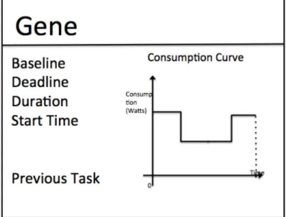
Figure 3.7 shows a possible representation of a chromosome that contains a set of genes. A gene is the smallest representation in an Evolutionary Algorithm. In this research, it represents a schedulable, non-preemptive task because at this time even preemptive tasks are divided into its sub-tasks, which are, as said previously, non-preemptive. Within this gene there is all the information regarding the task. Details about the information contained within each gene can be found in 3.1.1.

One very important value contained into the gene is the tasks’ start time. It is crucial that the start time of the task is calculated in a good direction because the overall fitness of the schedule depends on this value. Subsection 3.2.4 explains with detail the generation of a task’s start time within a specific schedule.

Figure 3.8: Gene Representation.

3.2.3 Population Generation

In this research the generation of the population is straight forward, generating a total of 100 individuals. Initial population has a minimum 70% of valid individuals to enable faster results,

(39)

avoiding having a majority of invalid individuals as much as possible. While avoiding this major-ity, some invalid individuals can also be useful in improving the solution, given the evolutionary nature of the algorithm. This also enables a good balance between the quality of the population and generation time, since providing valid chromosomes can be much slower than randomly providing one (valid or invalid), depending on the number of genes in the chromosome.

The generation of the initial individuals depends on pricing and tasks to perform. With this information, individuals can be generated, gene by gene with the knowledge of each task’s infor-mation to calculate its start time. The calculation of each new start time is explained in depth in subsection 3.2.4.

3.2.4 Start Time Calculation

In order to reach the optimal solution, each task calculates its own start time using the pricing intervals given to the scheduler. After receiving the pricing array, a rather complex algorithm is used to choose, stochastically, the best start time for the task. It starts by checking if the task has any preceding task, to avoid overlap between chunks in preemptive tasks. Note that the first sub-task in each preemptive sub-task is recognized as a non-preemptive sub-task, since it has no predecessor, so its start can be the task’s baseline. At this initial point every task has its time window ending at the deadline.

After obtaining the first time boundaries found, and in order to avoid further unnecessary processing, if the available time for running the task is equal to the task’s duration, the start time will be equal to baseline.

Until this point, there is not much calculation since time restrictions do not allow any heuristic. After this stage, start time calculation requires aid from the electricity pricing to calculate which start time should be used. As mentioned previously, electricity pricing plays a role on informing when producers want the customers to use energy in order to avoid peak demand. This could be easily achieved by choosing the cheapest pricing frame within the task’s baseline and deadline. However, these actions can lead to a problem of energy starvation since the power required for running all tasks that can be executed within that price time frame, might be higher than the available electricity.

In order to avoid electricity starvation, each task must know what are the pricing frames where it can be running.

Narrowing the domain to only valid time frames, as seen in Figure 3.9 enables performance, but since it is very simple, something more must be done. Before going further into the computa-tion of a task’s start time, we must check if the task is only eligible for one price frame.

3.2.4.1 One Pricing Frame

On pricing frame means that due to task’s time specification and pricing time frames, the start time can only be chosen into only one electricity price. Therefore, there is no argument in differentiat-ing each possible start minute because, in terms of pricdifferentiat-ing, they represent the same price. So, at

(40)

Figure 3.9: Time Frames Choice.

this point the only concern is related to fine tune each start time in order to enable a best overall schedule. For instance, each start time can lead to different electricity consumption curves that can exceed the available power. In order to take all this into consideration, for one pricing frame we run the following algorithm:

Algorithm 2 Start time calculation with one pricing frame.

1: start← thisTask.Baseline 2: end← thisTask.DeadLine 3: if (thisTask.hasPreviousTask) then 4: start← previousTask.EndTime 5: else 6: if (random(10) < 5) then 7: StartTime← start

8: StartTime← start + randomMinute(end − start − thisTask.Duration)

9: end if

10: end if

Algorithm 2 shows that in, 50% of the times the start time is the task’s baseline or preceding task’s end time, if the task is part of a preemptive task. The other 50% of times a random start time is chosen within the possible minutes without ending the task after deadline.

3.2.4.2 More than One Price Frame

Having more than one pricing frame brought the need for choosing between the possible ones. In this research a probabilistic method is used that enables choosing between the different prices. This method is often called Roulette Wheel Selection [LL12, Cen13]. This heuristic enables a probabilistic choice between possible prices in order to favor cheapest pricing time frames. This choice was made because of performance issues. As said previously, since the time unit chosen

(41)

was 1 minute, search space can be big and consequently make schedule search slow. Knowing this, there is more chance in finding the best schedule by assigning each task to cheapest pricings. This cannot be hard-ruled since it can lead to a probable state of energy shortage and impossibility of performing schedules. Instead, Roulette Wheel Selection makes possible to address with higher priority the cheapest price without compromising power validation, making possible the choice of a second cheapest price and so on, if needed.

In order to choose the starting time the ratio between each price and the sum of all pricing values is calculated. These ratios are used to give a probability of each interval to be chosen. Higher probability values are given to cheapest pricing intervals. The following example illustrates this process.

For one given task, the possible price frames are the following:

0.1AC / kW/h 0.3AC / kW/h 1.1AC / kW/h 0.5AC / kW/h

After identifying the possible pricing frames, the weight of each one within the sum of all prices is calculated. Formula 3.1 calculates the weight value of each pricing.

weight(pricei) =

price(i) ∑NPricest=1 price(t)

(3.1)

For this example, the result of the previous equation will result in the following. Price 0.1AC / kW/h 0.3AC / kW/h 1.1AC / kW/h 0.5AC / kW/h

Weight 0.05 0.15 0.55 0.25

Probability 55% 25% 5% 15%

In order for these weight values to be applied as the probability of each price to be chosen, they must be assigned to each price sideways, assigning to the cheapest price, the weight of most ex-pensive price frame. This assigning operation is performed by an auxiliary algorithm. Figure 3.10 shows the metaphor behind this process.

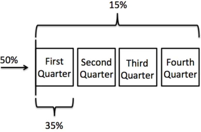
After choosing a price frame, start time calculation checks if the duration of the task is equal to the pricing duration. If true, the returning value is the pricing’s start time. If not, the start time calculation proceeds by calculating if the task duration is not higher than pricing’s duration. If it is, tasks’s start time is calculated by using all of pricing duration and 50% of times it chooses to anticipate start time to previous pricing, while other 50% of times it chooses to delay to next pricing. If the task is still bigger than available time frame, it repeats the same decision until the task fits into the time frame. This proceeding occurs only if task’s baseline or deadline are not violated.

On the other hand if the task’s duration is smaller than the pricing duration, the decision is divided by 3 methods. The first one returns the later time between task’s baseline and pricing start time in 50% of times. With 35% of chance is chosen a random minute within the first quarter

(42)

Algorithm 3 Start Time Calculation For More That One Time Frame.

1: price← RouletteW heel(AllPrices)

2: if (start < price.StartTime) then

3: start← price.StartTime

4: end if

5: if (end > price.EndTime) then

6: end← price.EndTime

7: end if

8: domain← end − start − thisTask.Duration

9: if domain < 0 then 10:

11: if end - domain <= thisTask.Deadline && start + domain >= thisTask.BaseLine then

12:

13: if random(10) < 5 then

14:

15: return end - domain

16: else

17: return start + domain

18: end if

19: end if

20: else

21:

22: if (end - domain <= deadline) then

23:

24: return end - domain

25: end if

26:

27: if (start + diff >= liveline) then

28:

29: return start + domain

30: end if

(43)

Figure 3.10: Roulette Wheel Selection.

of domain. The final 15% of times, start time is chosen as a random minute within domain. Figure 3.11 shows a visual representation of which probability is assigned to each part of the task.

Figure 3.11: Start Time Probabilistic Choice Within Possible Domain.

Concluding, this last nuance of calculating start time is implemented by following algorithm. The performance of this algorithm is deeply connected to maximizing overall performance of the whole scheduling algorithm since it focus on giving more importance to some time chunks of the domain, which they are more likely to contribute to a best overall schedule.

3.2.5 Crossover

After population generation, the evolutionary algorithm starts manipulating individuals in order to generate fitter individuals. One of the operations performed is called crossover. This crossover operation resembles biological crossover by creating new individuals with genetic combinations of its parents. Computational crossover relies precisely in the same method, combining fittest genes from each chromosome, generating a better individual.

(44)

Algorithm 4 Start Time Calculation If Task’s Duration is Smaller Than Pricing Duration. price← RouletteW heel(AllPrices)

if (start < price.StartTime) then start← price.StartTime end if

if (end > price.EndTime) then end← price.EndTime end if

domain← end − start − thisTask.Duration if domain >= TWOMINUTES then

if (random.nextInt(10) < 5) then return start else if (random.nextInt(10) < 7) then return random(firstQuarterOf(domain)) end if end if else

return start + random.nextInt(domain) end if

There are many computational methods to perform crossover such as one-point crossover or two-point crossover [JS92]. Despite the existence of these methods they did not fit as a first choice for this problem. One and two point crossover need many iterations to create new chromosomes that can be better than its parents in this particular problem. Also they can easily violate available power and task precedences.

For the sake of this research, another non elitist crossover method was created in order to enhance performance. This crossover method speeds up the generation of good chromosomes by interlacing all genes to form two new chromosomes. After Crossover the first child chromosome contains the cheapest genes between the two parents and second chromosome receives the most expensive genes. At this stage no power or precedence validation is made. In case of existing preemptive tasks, each generated chromosome is analyzed and for each preemptive task that starts before its predecessor is calculated a new start time to prevent precedence failures. After that, two fittest chromosomes from initial four are chosen and reintroduced into the population.

The crossover method is repeated, combining the most fit chromosomes in order to help find-ing the optimal solution for each schedulfind-ing problem. One of crucial factors for crossover to be successful resides in the choice of parent chromosomes since they are the origin of child chromo-somes that bring better solutions.

(45)

3.2.5.1 Chromosome Selection

There is higher probability of finding very good solutions if the right chromosomes are chosen to be crossed. The method chosen for selection in this research is not very common but since the results must be reached within a small time frame, more complex choosing methods must be avoided.

Selection in this research is performed in a very simple way. When choosing candidates, there are 50% chances of choosing the best individual to cross with another random individual. In other 50% of times two random individuals are chosen. With this random choice computational expenses are low, since there is no need to calculate any type of probabilistic choice regarding the fitness of each chromosome in the population. Also, improving the best chromosome with other random chromosomes has shown to be a very good vehicle to reach optimal solutions, from the fact that search space can be large.

Next, the fitness evaluation function that quantifies how good is each individual.

3.2.6 Fitness Function

The fitness function is used to analyze chromosomes and measures its level of “goodness”. With this feature it is possible to compare or select chromosomes during the whole execution of the evolutionary algorithm. First of all, there is the need to define what factors are important and contribute in each chromosome for its fitness. The fitness function defined for this research takes into account three factors:

• Schedule Price Sum of every task cost, taking into account the prices during task’s execu-tion time;

• Task Precedences The number of precedence failures on preemptive tasks;

• Power Usage Validation The number of minutes that consumption of all tasks is above the available power.

In order to deeply understand the fitness function, each factor is explained next.

3.2.6.1 Schedule Price

One of three factors in fitness function is the cost of each task. Since price of energy is not constant, neither task’s start time, each task will have a different cost on each different schedule. With this being said, equation 3.2 calculates the cost of one entire schedule.

Cost= AllTasks

∑

i=1 ( StartTime+TaskDuration

∑

t=StartTime

(46)

The cost is calculated by adding each multiplication of task’s consumption at each minute and price of energy at each minute of the day that the task is running.

3.2.6.2 Task Precedences

Another factor that contributes for the fitness value is preemptive tasks’ parts precedences. This factor is only taken into account if the schedule figures preemptive tasks. All preemptive tasks are Finish to Start, meaning that each task start time depends on previous task end time. There also can be a lag > 0 between each task. In order to guarantee this rule to be met, algorithm 5 validates it.

Algorithm 5 Task’s Precedence Calculation. for all Tasks in Chromosome do

if (Task.HasPreviousTask) then

if (Task.PreviousTask.EndTime > Task.StartTime) then PrecedenceErrors++

end if end if end for

return PrecedenceErrors

3.2.6.3 Power Usage Validation

Power usage validation checks if in any scheduled minute the power usage, being the sum of each task consumption in that minute, is exceeded. Alike task precedences, this factor is only taken into account if the sum of maximum energy consumption of each task, between their baseline and deadline, is below the available power.

for time = FirstTask.StartTime to LastTask.EndTime do consumption← 0

for all Tasks task in Chromosome do

if ((time >= task.StartTime) && (time < task.EndTime)) then consumption += task.getConsumption(time)

end if end for

if (consumption > AvailablePowerAt(time)) then ConsumptionErrors++

end if end for

return ConsumptionErrors

The fitness function combines these previous explained factors in order to generate a value that categorizes each chromosome. Despite of being electricity the real cost for the customer, it is the least important in the fitness function because the other two factors are heavily penalizing since if their value is above zero in any of those factors, the schedule will be impossible to execute.