Decision support system for city public transportation

Universidade de Aveiro Departamento deElectr´onica, Telecomunica¸c˜oes e Inform´atica, 2017

Leandro

Ricardo

Sistema de Suporte `

a Decis˜

ao para Transportes

P´

ublicos

Decision Support System for City Public

Transportation

Universidade de Aveiro Departamento deElectr´onica, Telecomunica¸c˜oes e Inform´atica, 2017

Leandro

Ricardo

Sistema de Suporte `

a Decis˜

ao para Transportes

P´

ublicos

Decision Support System for City Public

Transportation

Disserta¸c˜ao apresentada `a Universidade de Aveiro para cumprimento dos re-quisitos necess´arios `a obten¸c˜ao do grau de Mestre em Engenharia de Com-putadores e Telem´atica, realizada sob a orienta¸c˜ao cient´ıfica da Professora Doutora Susana Sargento, Professora Associada com Agrega¸c˜ao do De-partamento de Eletr´onica, Telecomunica¸c˜oes e Inform´atica da Universidade de Aveiro e co-orienta¸c˜ao cient´ıfica do Professor ´Ilidio Oliveira, Professor Auxiliar do Departamento de Eletr´onica, Telecomunica¸c˜oes e Inform´atica da Universidade de Aveiro.

o j´uri / the jury

presidente / president Professor Doutor Jos´e Manuel Matos Moreira

Professor Auxiliar do Departamento de Eletr´onica Telecomunica˜oes e Inform´atica da Universidade de Aveiro

vogais / examiners committee Professor Doutor Pedro Miguel Alves Brand˜ao

Professor Auxiliar do Departamento de Ciˆencia de Computadores da Faculdade de Ciˆencias da Universidade do Porto

Professora Doutora Susana Isabel Barreto de Miranda Sargento Professora Associada com Agrega¸c˜ao do Departamento de Eletr´onica Telecomu-nica˜oes e Inform´atica da Universidade de Aveiro (orientadora)

agradecimentos / acknowledgements

No culminar do meu percurso acad´emico n˜ao me poderia esquecer de agradecer a todas as pessoas que contribuiram para o meu sucesso. Em primeiro lugar, agrade¸co aos meus pais Jorge e Elisabete e aos meus irm˜aos Rita e Francisco, por todo o amor, carinho e apoio incondicional.

`

A minha namorada, Maria Ant´onio, por todas as horas de paciˆencia e carinho.

Aos meus amigos, Nuno Henriques, Marco Silva, Cristina Silva, Rui Pedro, David Silva, Eduardo Sousa, Mafalda Rodrigues, Al´exio Sim˜oes, Daniela Sousa, Jo˜ao Sim˜oes e Jos´e Moreira pelo companheirismo e amizade que concerteza permanecer˜ao durante muito mais anos.

`

A minha orientadora, a incans´avel Susana Sargento, que al´em de me ter dado a oportunidade de colaborar num grupo de investiga¸c˜ao relevante e me ter ajudado com todos os problemas recorrentes do desenvolvimento deste trabalho, me incentivou e inspirou a pensar e a desenvolver trabalho com impacto.

Ao meu co-orientador, Il´ıdio Oliveira, pelas suas sugest˜oes, opini˜oes e vis˜ao, ajundando-me a melhor reflectir sobre os problemas deste trabalho.

Ao professor Jos´e Maria Fernandes, pelas suas sugest˜oes e infind´aveis ideias. Ao Jorge Pereira e Bruno Areias colegas do grupo de investiga¸c˜ao que apesar de terem tamb´em os seus problemas, arranjaram sempre um tempinho para me ajudar com os meus.

Aos investigadores postdoc do grupo de investiga¸c˜ao, em particular ao Miguel Lu´ıs, pelas suas cr´ıticas extremamente assertivas e construtivas, ao Carlos Senna pela sua partilha de experiˆencia e ao Lucas Guardalben.

Resumo Hoje em dia existe tecnologia para tornar as cidades inteligentes. As cid-ades inteligentes s˜ao capazes de sentir, analizar e reagir: sentir atrav´es dos variados sensores espalhados em torno da cidade, sensores estes que podem ser fixos (sensores para a monitoriza¸c˜ao do estado ambiental) ou m´oveis (por exemplo, os cidad˜aos, gra¸cas aos seus smartphones). Um caso not´avel ´

e o da cidade do Porto, que incorpora uma rede em malha com mais de 600 ve´ıculos (autocarros, taxis e cami˜oes do lixo) que comunicam entre si, habilitando os passageiros dos autocarros da maior operadora da cidade a navegar na internet gratuitamente, enquanto viajam.

O maior impacto de uma rede como esta ´e a mobilidade; e uma das pre-ocupa¸c˜oes das institui¸c˜oes governamentais locais ´e como elas podem mel-horar a mobilidade.

´

E por isso crucial analisar o que pode ser feito para melhorar a mobilidade de uma cidade. Utilizando os dados gerados pelo movimento dos autocarros ´

e poss´ıvel fornecer um conjunto de novas utilidades pr´aticas que podem ser ´

uteis ao quotidiano dos cidad˜aos e dos gestores de frota. Na perspetiva dos passageiros pode ser introduzido o conceito de smart schedule que consiste em fornecer o tempo estimado de chegada de um autocarro que se vai adaptando ao longo do tempo, de acordo com a dinˆamica da cidade, que pode ser acedido diretamente a partir do seu smartphone. Na perspetiva dos gestores de frota ´e poss´ıvel fornecer introespe¸c˜oes sobre o comportamento habitual das linhas de autocarros, dando abertura a que estes sejam capazes de melhor reagir a novas ou anormais dinˆamicas dos transportes p´ublicos da cidade.

Esta disserta¸c˜ao apresenta uma abordagem para analisar os dados proveni-entes da rede veicular e de como us´a-los para tornar as ideias previamente esclarecidas, poss´ıveis. Devido `a inexistˆencia da identifica¸c˜ao do tra¸co GPS a uma linha de autocarro, um algoritmo de map-matching foi implementado. Isso torna a computa¸c˜ao de estima¸c˜oes e predi¸c˜oes sobre o tempo de pas-sagem dos autocarros poss´ıvel. No que toca `a predi¸c˜ao, foram testados trˆes algoritmos diferentes de aprendizagem autom´atica em conjunto para a constru¸c˜ao de modelos preditivos. Por fim, foram implementadas aplica¸c˜oes como prova de conceito que demonstram a aplicabilidade no mundo real, ajudando os passageiros dos autocarros e os gestores de frota a reagir aos diferentes eventos do seu quotidiano.

Os resultados demonstram que o algoritmo de map-matching apresenta uma boa qualidade. Tamb´em demonstram que o melhor algoritmo de aprendiz-agem autom´atica, considerando o erro de predi¸c˜ao, ´e o Bagging utilizando como estimador base Support Vector Regressor. Por fim, os perfis obtidos pelo painel de controlo permitem distinguir linhas de autocarro com um funcionamento ´otimo daquelas em que o funcionamento ´e insatisfat´orio.

Abstract Nowadays, the technology to turn cities smart already exists. Smart Cities, as they are called, are capable to sense, analyze and react: sense through the set of sensors displaced along the city, as they are sensors either fixed (for environmental monitoring) or moving (for instance, citizens with their smartphones). A notable case is Porto, which incorporates a mesh network with more than 600 vehicles (buses, taxis and garbage trucks), communic-ating in-between and enabling the passengers of the buses of the city major bus carrier to access freely to the Internet while commuting.

A vehicular network like this has huge positive impact in the city mobility, which is one of the biggest concerns of the governmental institutions. Therefore, it is crucial to understand what can be done to improve mobility. By analyzing the data generated by the movement of the buses, it is possible to deliver a new set of tools that might be useful for the everyday life of the bus passengers and bus fleet managers. From the passengers perspective, the utility can be brought by the introduction of smart schedules, which consists on delivering estimated time of arrival that is adapting itself to the city dynamics, through the evolution of the time, and that can be accessed directly from their smartphones. From the perspective of the bus fleet managers, it is possible to deliver insights about the usual behaviour of their bus lines, giving openness for them to react to the new or abnormal city public transportation dynamics.

This dissertation presents an approach for analyzing the data descendent from the vehicular network and how to use it to answer the previously ad-dressed problems. Regarding the missing link between the GPS trace from the bus and the bus line that they are doing, a map-matching algorithm is implemented. That turns possible the computation of estimations and predictions of the bus’ passing times. In what concerns prediction, three machine learning ensemble algorithms have been tested. Finally, proof-of-concept applications are implemented to demonstrate the real-life applicab-ility, by helping the bus passengers and bus fleet managers to react to the different events of their quotidian.

The results show that the map-matching algorithm presents a good quality. Also, they demonstrate that the best machine learning algorithm, consider-ing the prediction error, is Baggconsider-ing usconsider-ing Support Vector Regressor as the base estimator. Finally, the profiles obtained in the performance dashboard enable distinction between optimal and non-optimal bus lines.

Contents

Contents i

List of Figures v

List of Tables vii

Acronyms ix 1 Introduction 1 1.1 Motivation . . . 1 1.2 Objectives . . . 2 1.3 Contributions . . . 3 1.4 Acknowledgments . . . 3 1.5 Document outline . . . 3 2 Concepts 5 2.1 Introduction . . . 5 2.2 Smart Cities . . . 5 2.2.1 Definition . . . 5 2.2.2 Challenges on mobility . . . 7 2.3 Vehicular Networks . . . 7 2.3.1 Definition . . . 7

2.3.2 Importance of VANET under the context of this work . . . 9

2.4 Fundamentals of mapping . . . 10

2.4.1 Introduction . . . 10

2.4.2 The shape of the earth . . . 10

2.4.3 Datums and projections . . . 11

2.4.4 Issues regarding spatial data handling . . . 13

2.5 Data processing fundamentals . . . 13

2.5.1 Introduction . . . 13

2.5.2 Concurrent, parallel and distributed computing . . . 13

2.5.3 Big Data definition and characteristics paradigms . . . 14

Big Data processing Paradigms . . . 15

2.6 Machine Learning . . . 16

2.6.1 Definition . . . 16

2.6.2 Types of Machine Learning . . . 17

Unsupervised Learning . . . 18

Reinforcement Learning . . . 18

2.6.3 Fundamental concepts . . . 19

Machine Learning Workflow . . . 19

Generalization, Overfitting and Underfitting . . . 20

Model Selection and Cross-Validation . . . 20

Improving models performance with Ensemble Learning . . . 21

2.7 Summary . . . 22

3 Related Work 25 3.1 Introduction . . . 25

3.2 Bus Trajectory Identification by Map-Matching . . . 25

3.3 Comparing state-of-the-art regression methods for long term time prediction . 26 3.4 Empirical Study of Travel Time Variability Using Bus Probe Data . . . 27

3.5 Using Bus Probe Data for Analysis of Travel Time Variability . . . 28

3.6 A review of travel time estimation and forecasting for Advanced Traveller In-formation Systems . . . 30

3.7 Real-time Trip Planner in Urban Public Transport . . . 32

3.8 Summary . . . 33

4 Matching lines with GPS logs and Building Performance Indicators 35 4.1 Introduction . . . 35

4.2 Problem Setting . . . 35

4.3 Available Context . . . 36

4.3.1 Data Sources . . . 36

4.3.2 Insights on the log database . . . 36

Database Tables . . . 36

A detailed view on node data: attributes, granularity, quality and quantity . . . 37

4.3.3 STCP Website as data source . . . 38

4.4 Exploring, visualizing and choosing data . . . 38

4.4.1 Position Log Data . . . 39

4.4.2 Bus network data description . . . 39

4.5 Performance Indicators . . . 41

4.5.1 Definitions . . . 41

4.5.2 Main restritions . . . 42

4.6 Summary . . . 42

5 Architecture and Technical Design 43 5.1 Introduction . . . 43 5.2 Requirements . . . 43 5.2.1 Functional requirements . . . 43 5.2.2 Non-functional requirements . . . 44 5.3 Architecture . . . 44 5.4 Technical Design . . . 46 5.4.1 Overview . . . 46

5.4.3 Algorithm Design . . . 49

Making spatial searches . . . 50

Using and choosing a detection radius . . . 50

Detecting line starts . . . 52

Finding a solution . . . 52

5.4.4 Building performance indicators . . . 57

A deeper overview on completeness metric . . . 57

Estimating arrival times . . . 57

Predicting arrival times . . . 59

5.5 Summary . . . 60

6 System Implementation 61 6.1 Introduction . . . 61

6.2 Bus Network Information Retrieval . . . 62

6.2.1 Script to retrieve base data implementation details . . . 64

6.2.2 Script to transform base data implementation details . . . 65

6.3 Matching Unit . . . 66

6.3.1 Development History . . . 66

6.3.2 Overview . . . 67

6.3.3 Modules . . . 67

6.3.4 The entities module . . . 68

Worker implementation overview . . . 68

Dispatcher implementation overview . . . 69

Logger implementation overview . . . 69

6.3.5 The pipeline module . . . 69

Algorithm to detect when a line starts . . . 70

Algorithm for finding solutions from line starts . . . 70

6.3.6 The tools module . . . 73

6.4 Matches Database . . . 73

6.4.1 Overview . . . 73

6.4.2 Database schema description . . . 74

6.4.3 Routines . . . 75 6.4.4 Functions . . . 75 6.5 Estimation Database . . . 76 6.5.1 Overview . . . 76 6.5.2 Development history . . . 76 6.5.3 Database diagram . . . 77

6.5.4 Database schema description . . . 77

6.5.5 Routines . . . 78

Functions . . . 78

Triggers . . . 80

6.5.6 How estimates are calculated . . . 80

6.6 Synchronization Script . . . 80

6.7 Prediction Module . . . 81

6.7.1 Overview . . . 81

6.7.2 Algortihms . . . 81

Requirements . . . 82

Dataset characterization . . . 83

6.7.4 Model Selection and Cross Validation . . . 83

6.7.5 Evaluation . . . 84

6.7.6 Deployment . . . 85

6.8 Database Wrappers Module . . . 85

6.9 Integration APIs . . . 85

6.9.1 Bus Network Information API . . . 86

6.9.2 Match API . . . 87

6.9.3 Estimation API . . . 87

6.9.4 Prediction API . . . 87

6.10 Applications . . . 87

6.10.1 Bus Line Performance Dashboard . . . 88

6.10.2 Bus Passenger Mobile Application . . . 89

6.11 Summary . . . 90

7 Deployment and Results 93 7.1 Introduction . . . 93

7.2 Deployment . . . 93

7.2.1 Hardware . . . 93

7.2.2 Software . . . 93

7.3 Results . . . 95

7.3.1 Matching GPS traces with bus lines . . . 95

Context . . . 95

Processed Data in numbers . . . 95

Results presentation . . . 95

Analysis and Validation . . . 96

7.3.2 Delay metrics for bus lines and estimated times of arrival . . . 98

Context . . . 98

Result presentation 1.1: Delay plot of a bus line match . . . 98

Result presentation 1.2: Detecting problematic lines . . . 102

Result presentation 2: Estimated time of arrival given a previously defined static value from the STCP time tables . . . 103

Result presentation 3: Estimated time of arrival given a dynamically chosen value (user given or inferred by the delay plot analysis) 104 Validation . . . 104

7.4 Prediction Module Results . . . 104

7.4.1 Regression Metrics Comparison . . . 105

7.5 Summary . . . 107

8 Conclusion and Future Work 109 8.1 Conclusion . . . 109

8.2 Lessons Learned . . . 109

8.3 Future Work . . . 112

List of Figures

1.1 A figurative image of a smart city . . . 1

2.1 A vehicular network and its interactions . . . 8

2.2 Vehicular Network Architecture (figure from Andre Cardote) . . . 9

2.3 The earth Geoid GOCE (ESA/HPF/DLR) . . . 11

2.5 A standard Lambda Architecture, its modules and methodologies, presented by the company MapR [23] . . . 16

2.6 An example of classification task distinguishing cats from dogs [26] . . . 17

2.7 An example of a clustering task, which distinguished 3 different groups [26] . 18 2.8 The typical machine learning workflow [26] . . . 19

2.9 Presentation of the relation between the model complexity and the model pre-diction error (taken from [14]) . . . 21

2.10 Majority voting used in a machine learning ensemble method (taken from [33]) 22 3.1 Comparison of the different time periods in terms of stability [6] . . . 28

3.2 Data transformation steps described by Uno et al. [45] . . . 29

3.3 Traffic data sources. (a) Point detectors, (b) probe vehicles and (c) Interval detectors (figure from the review [28]) . . . 31

3.4 ”Difference between time travel estimation and prediction”[28] . . . 32

3.5 NextBus Architecture (figure from [3]) . . . 33

4.1 An all day long position Log from a bus from the first day of March . . . 40

4.2 Bus stops of Porto . . . 40

4.3 Bus lines of Porto . . . 41

5.1 Architecture components and the data flow . . . 45

5.2 Data Processing Pipeline . . . 46

5.3 Matching Unit Architecture . . . 47

5.4 Worker Design Pattern Design . . . 48

5.5 A non-ideal and an ideal radius . . . 51

5.6 The stop S has two lines starting in its position. If the bus is passing near that position S, there is a probability that one of the lines starting there is the solution. . . 52

5.7 Detect line starts algorithm . . . 53

5.8 Algorithm phases . . . 54

5.9 Matching Algorithm Flowchart . . . 56

6.1 Line Details Page from STCP Website . . . 62

6.2 Capture on Wireshark showing the filter and the HTTP GET Requests to the STCP API . . . 63

6.3 Matching Unit Modules . . . 68

6.4 Matches Database Diagram . . . 74

6.5 Data Mart Diagram . . . 76

6.6 Data Mart Diagram (not definitive image) . . . 77

6.7 TimeSeriesSplit iterations over data . . . 82

6.8 User Interface of Matches API, generated by Swagger . . . 86

6.9 This is the match browser view, where the bus fleet manager can analyze each one of the matched bus journeys. . . 89

6.10 A view over the delay plot . . . 89

6.11 Two different views of the mobile application . . . 91

7.1 The match from the node id 2764 from March, 1 St, from 07h00m to 07h55m, with 100% completeness. . . 96

7.2 The match from the node id 2474 from March, 15 St, from 14h32m to 15h19m, with 100% completeness . . . 96

7.3 The match from the node id 2801 from March, 8 St, from 18h10m to 19h17m, with 91% completeness due to gaps on the input records from the position log database, outlined with stroked circles. . . 97

7.4 A line completion with uncertainty . . . 98

7.5 Line 204 Hospital de S. Jo˜ao from 07:01:33 to 07:53:48 . . . 100

7.6 Line 204 Hospital de S. Jo˜ao from 07:57:50 until 09:02:20 . . . 100

7.7 Line 204 Hospital de S. Jo˜ao from 12:01:05 until 12:56:51 . . . 100

7.8 Line 204 Hospital de S. Jo˜ao from 15:03:36 until 15:59:51 . . . 101

7.9 Line 204 Hospital de S. Jo˜ao from 17:26:37 until 18:44:52 . . . 101

7.10 200 Castelo do Queijo, 3 months analysis . . . 102

7.11 204 Hospital de S. Jo˜ao, 3 months analysis . . . 102

7.12 902 Boavista, 3 months analysis . . . 103

7.13 Bagging (using support vector regressor) . . . 106

7.14 Random Forrest . . . 106

7.15 Gradient Boosting . . . 107

List of Tables

3.1 Time Periods from this study[6] . . . 28

4.1 Description of the attributes of the table node data . . . 37

7.1 Statistics for a time query associated to a bus line and bus stop . . . 103

7.2 Statistics for a time query associated to a bus line and bus stop . . . 104

Acronyms

API Application Programming Interface. 45, 61–63, 83, 85–90, 94, 104, 107 CPU Central Processing Unit. 44, 47, 66

ESA European Space Agency. 11

GOCE Gravity field and steady-state Ocean Circulation Explorer. 11

GPS Global Position System. 2, 3, 7, 11, 12, 23, 25, 28–30, 33, 35, 37, 39, 49–51, 54, 55, 57, 104

HTTP Hypertext Transfer Protocol. 63, 65

ICT Information and Communication Technologies. 23 JSON JavaScript Object Notation. 64, 65, 67, 87 LMA Local Mobility Anchor. 9

MAG Mobile Access Gateway. 9

MIT Massachusetts Institute of Technology. 33 mMAG Mobile MAG. 10

MNN Mobile Network Node. 10 NoSQL Not-Only SQL. 15, 111 OBU On-Board Unit. 10, 37 RAM Random Access Memory. 44 SMS Short Message Service. 2

SQL Structured Query Language. 73, 75, 79, 85 SSD Solid-State Disk. 44

STCP Sociedade de Transportes Colectivos do Porto. 2, 9, 27, 38–40, 44, 46, 57, 62–64, 90, 94, 95, 98, 99, 103, 104, 108

SVM Support Vector Machine. 20 TETRA Terrestrial Trunked Radio. 27 TTL Time To Live. 70, 71

TTP Travel Time Prediction. 26 URL Uniform Resource Locator. 63

VANET Vehicular Ad-hoc Networks. 2, 7–9 WGS World Geodetic System. 11

Chapter 1

Introduction

1.1

Motivation

In the last several years, the term Smart City has been acknowledged, first by the re-searchers, then by the governments, and finally by the people.

As a multidimensional concept, Smart City covers a wide range of equally smart topics: green city (related to smart profiteering of the environmental resources), the smart growth (related to a human-aware and sustainable urban development), the smart grid (related to efficient electrical energy delivering), etc.

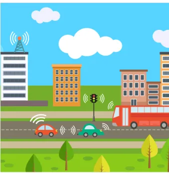
These topics are intersected between them, and they have a thing in common: they look to enhance the people’s life through the use of the technology. The Figure 1.1 depicts this relation.

Figure 1.1: A figurative image of a smart city

the city and commuting is, for some, a significant part of their everyday life. Therefore, the concept of Smart Transportation becomes apparent and answering to the question ”how can cities improve their public transportation system” becomes a top priority.

Regarding mobility and the smart transportation topic, an accessible case-study can be further explored. Porto, the second largest city in Portugal after Lisbon, is a Smart City, and it deploys a world-level pilot project which implements a Vehicular Ad-hoc Networks (VANET) connecting buses, garbage trucks and taxis. This mesh network is capable of deliv-ering free wireless internet access to bus passengers, enhancing their commuting experience. One may ask what can be done for enhancing further the commuting experience.

Thinking about the impact of the existing applications in everyone daily life, Sociedade de Transportes Colectivos do Porto (STCP), which is the major Porto’s bus carrier, provides a service called SMSBUS. It delivers estimated times of arrival for a given line or bus stop, recurring to the sending of a Short Message Service (SMS). Unfortunately, it is a paid ser-vice1and it depends on specific and expensive requirements (like using antenna triangulation). Regarding the existing framework (the vehicular network), it may be possible to produce mobile applications with the objective of delivering bus line schedules, routes and others for free. Also, it would be interesting if it was possible to provide customer oriented services enabling bus passengers to subscribe a bus stop and querying for delays, which could be dy-namic, depending on the past history (estimated time of arrival) and on the current traffic (prediction of the time of arrival).

Predicting the bus route behavior in terms of delay is relevant for the bus carrier managers, in the scope of understanding if there are problems due to road works, bus route congestion, and other events that may interfere, even despite of the existence of proprietary systems, in production for years.

Therefore, the answer may live on optimizing the way the passengers commute, poten-tially by increasing the knowledge about the behaviour of the buses. This may be possible through the development of a mobile application concerning a map of bus stops, bus lines, and schedules which could be estimated, using the past history. On the other hand, bus carriers are constantly looking for optimizing the way they manage their resources, being absolutely essential for them to understand how is their bus carrier performing in a particular bus line. Given the data resulting from the operation of the network, like the movement of the nodes in space (GPS position, velocity, etc), it is possible to tackle these specific problems. The motivation of this work is to make use of the network operation data for optimizing the way bus passengers commute, and optimize also, the way bus carrier managers perceive the bus network behavior.

1.2

Objectives

Given the previously exposed problems, the main purpose of this dissertation is to:

• Create a solution for obtaining the bus estimated times of arrival in a given line and stop (or a set of stops), based on the past history.

• Regarding the first objective, solve the missing link between the position log data and the bus network infrastructure because it is not possible to know which bus was completing a given line. This will require matching the Global Position System (GPS) trace of the buses with a bus line.

• Using machine-learning techniques on historical data, predict the bus behavior, in terms of delay, in the days to follow.

• Deliver proof-of-concept applications as they are an important step on extracting some results and on generating real life examples and tests.

1.3

Contributions

Following this study development, two articles have been submitted, with the same title ”Decision Support System for City Public Transportation”.

The first submission was targeted to INForum 2017, in October 12th and 13th, as a communication. It was accepted and presented via oral presentation and poster.

The second submission was targeted to VEHITS 2018, in October 30th and it is waiting for approval.

1.4

Acknowledgments

This work was supported in part by National Funds through FCT - Funda¸c˜ao para a Ciˆencia e a Tecnologia under the project UID/EEA/50008/2013, in part by the IT Internal Project SmartCityMules and in part by the CMU-Portugal Program through S2MovingCity: Sensing and Serving a Moving City under Grant CMUP-ERI/TIC/0010/2014.

1.5

Document outline

This document is organized as follow:

• Chapter 1 is the introduction for the work.

• Chapter 2 focuses on explaining some fundamental concepts which are useful on un-derstanding some decisions.

• Chapter 3 presents some of the most relevant works and their fundamental ideas. • Chapter 4 explains the problem setting in further detail.

• Chapter 5 presents the architecture and the theory behind the implementation. • Chapter 6 presents the implementation of the components comprising the architectural

• Chapter 7 presents how can this system be deployed and discusses the results of this work.

Chapter 2

Concepts

2.1

Introduction

This chapter introduces the main concepts which are meaningful for this work, presenting definitions which provide ground for understanding the importance of enclosing paradigms and the most common terminologies.

We start by explaining what is a smart city and presenting its challenges on mobility. Then, due to the fact that this study is based on data collected from a vehicular network, this topic is addressed too.

The data descending from the vehicular network is spatial-temporal and it has considerable volume. Regarding this data nature, the fundamentals of mapping are presented as means for drawing attention to the impact of this data type into the information systems. On the other side, because the volume of the data raises some concerns on the processing times, the different data processing paradigms are presented, first by explaining the concepts of the concurrent, parallel and distributed computing and then, by presenting the data processing paradigms.

Finally, it is presented the fundamental concepts of machine learning, which is a way of extracting knowledge from data.

2.2

Smart Cities

2.2.1 Definition

”There is neither a single template of framing smart city nor a one-size-fits-all definition of smart city. ... The label smart city is a fuzzy concept and is used in ways that are not always consistent.” [29]

To better define what is a Smart City, one could understand it as a multidimensional representation of a generic city, with three main fronts [29][11]:

• Technology dimension. • Human dimension. • Institutional dimension.

The Technology Dimension borrows most of its meaning from the concept of Digital, Ubiquitous and Information City, and thus, it is objectively focused on the infrastructure.

The concept of Digital City focuses on the communication infrastructure and on under-standing how flexible, service-oriented, based on open standards and capable should it be for delivering innovative services for citizens, businesses and to the government.

The Ubiquitous is referred to the set of ubiquitous devices which can be available on the urban elements, either active or passive urban particles (people, public or private transport-ation, or buildings and infrastructure) and generate information which results from the state or interaction between these devices.

Finally, Information City refers to the characteristic of the city on being capable of ex-ploring and delivering information from local communities and systems, through the use of the Internet (not necessarily from web portals but also from other closer alternatives like mobile applications).

The Human Dimension focuses its meaning in child concepts like Creative, Learning and Knowledge City, which are subsequently related on human relations and on how can they improve a city as a whole.

Creative City concerns the view of the city as friendly environment for the development of the human and social infrastructure. Human infrastructure defines the set of human or-ganizations where people are engaged due to work or other activity (for example, through an association, a volunteer group, etc) while Social Infrastructure is about the people, their relationship and how they generate benefit from social capital i.e.., how human relations can ”generate benefits that flow from the trust, reciprocity, information, and cooperation associ-ated with social networks” [18].

Last but not least important, the Institutional Dimension is an umbrella definition which relies on the Smart Community and Smart Growth concepts to highlight governance among stakeholders and institutional factors for governance [29].

One strong definition for Smart Community ”was coined by a blue-ribbon panel of experts, created by the Canadian government in 1998, to provide advice on a potential national Smart Communities programme” [47]. They defined Smart Community as community with common or shared interests in which its members, organizations and/or governing institutions work with information technologies to transform their daily life in a positive and significant way, regardless of the community size [24].

From another perspective, Smart Growth and Green City are two related concepts. The first one, Smart Growth, is focused on strategies which promote the development and conser-vation of the citizens health and environment. The second defines city as green when it puts effort on designing itself to generate the lowest impact possible to the environment, minim-izing its resource consumption requirements (food, water, energy, etc) and greatly reducing the production of pollution (air, heat, gas emissions, noise, etc).

Thus, the concept of Smart City could be expressed as an urban development vision which tries to bring the best out from the cooperation between people (citizens, organizations and the government), infrastructures (telecommunications, transports, general purpose building like schools, bridges, etc) and policies (either environmental, either urban development ones) through the use of Information and Communication Technologies, that connects and empowers both.

2.2.2 Challenges on mobility

The previous subsection supports the idea that the”Smart City will be the future trend of urban development”[42]. Generally, the development of a smart city encompasses the last three dimensions, which can have a huge impact in the real life.

The umbrella term for the smart initiatives concerning the mobility is called ”Smart Mobility”. It is not only concerned on increasing the commuting speed of the people around the city, but also, with reducing the costs of commuting, improving people safety, reducing pollution (either by the reduction of the emissions, either by the reduction of the noise) and reducing traffic congestion. This definition was first employed by Benovolo et al [8].

These objectives are overlapped in-between, being part of the scope of the smart mobility concept, and also, under the scope of the Smart Transportation.

Smart Transportation is all about ubiquity. Taking ”good advantage of sensor network, the Internet of Things and other technical means” [42] a city can increase its intelligence (i.e., knowledge) about the way urban particles – citizens, buildings, transportation and communication – interact.

It is almost classic to think of this as mean for understanding more about traffic and public transportation in such a way that it is possible to establish a smart traffic manage-ment system, or a dynamic public transportation performance tracker which could provide performance metrics and dynamic schedules. Therefore, the concept of Smart Urban Man-agement arises.

Viewing citizens as urban particles is also a current vision. For example, SenseMyCity [36] points out some observations which make clear why citizens are good candidates as ”moving sensors”.

Citing the same work, it is observed that ”people treat smartphones as a second skin, having them around nearly 24/7 and constantly interacting with them” and also that they (smartphones) ”are equipped with a wide range of embedded sensors, like GPS for location, magnetometer, accelerometer, gyroscope”.

If one takes advantage of this huge sensor network, it is possible to go further and un-derstand how the mobility (or the lack of it) affects citizens and how they interact with the existing infrastructures.

In sum, it would be possible to deliver a myriad of solutions capable of delivering strong support for the integration between the different smart city areas of development (the urban planning, construction, management and operations) and providing a deep understanding how the smart urban ecosystem works.

2.3

Vehicular Networks

2.3.1 Definition

In the wide topic of the intelligent transport systems, vehicular networks have been one of the trending areas in the last several years. Vehicular Ad-hoc Networks (VANET) is a network development paradigm that makes use of ”inexpensive wireless local area network (WLAN) technology that connects notebook computers to each other and the Internet, and, with a few tweaks, install it on vehicles”[15].

Figure 2.1: A vehicular network and its interactions

The concept of VANET is more ”similar to the one applied on ad-hoc networks”[25], meaning that there is a dynamic/spontaneous creation of a wireless mesh network.

The effort of bringing such technologies to vehicles results in a unique environment which raises new opportunities, challenges and requirements:

• Vehicles communicating between each other directly and with the infrastructure, raise opportunities for developing a more safe and aware road network and for building a set of applications in diverse areas, like safety, marketing, etc. For example, one of the earliest applications of vehicular networks was delivering internet access.

• Current vehicles are able to reach high speeds and work in highly dynamic environ-ments, which can differ a lot in terms of connectivity, being reasons that can raise some challenges on modelling the communication infrastructure and the communication protocols.

• Several issues regarding the government concerns on privacy and security raise new requirements [15]. Also, the new applications can raise new demands regarding higher packet delivery rates and lower packet latency.

2.3.2 Importance of VANET under the context of this work

Porto, the second largest city in Portugal after Lisbon, is a living lab. Thanks to an alliance between IT1, UA2, UP3, VENIAM4, Porto Digital 5 and STCP6, it was possible to deploy a large dimension mesh network using the buses, taxis and garbage collection trucks for providing free WIFI access to bus passengers.

This mesh network is, objectively, a Vehicular Ah-hoc Network capable of exchanging big amounts of information. It is also capable of generating big amounts of heterogeneous data (for example, time-series or spatial data) related to the buses position and velocity, opening opportunities for the creation of new applications not only related with safety, but also, with mobility and other important smart city issues.

Regarding that, being familiar with the meaning of the components of the architecture and its terminologies is very important for extracting meaning from wrangling7 the data.

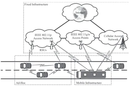
The figure 2.2 shows the Vehicular Network Architecture, as deployed on Porto.

IEEE 802.11p

Access Network Cellular Access_Network Internet Ad-Hoc Fixed Infrastructure RSUs Mobile Infrastructure IEEE 802.11g/n Access Points

Figure 2.2: Vehicular Network Architecture (figure from Andre Cardote)

The architecture of the VANET deployed i.e. Porto can be divided in four major com-ponents:

• Local Mobility Anchor (LMA): is the central component of the architecture that manages the IP mobility. It is located in one of the network machines (it could be either on a server, either on the cloud).

• Mobile Access Gateway (MAG): ”is a fixed infrastructure access point” [25]. It connects the mobile agents to the core of the network. A MAG can be a road side unit,

1

Instituto de Telecomunica¸c˜oes

2_{Universidade de Aveiro} 3

Universidade do Porto

4

A vehicular networks company (https://veniam.com/)

5

Porto Digital is a private association which promotes ICT projects within the context of Porto City and Porto’s metropolitan area (https://portodigital.pt/index.php?artigo=19)

6_{Porto’s major bus carrier (http://www.stcp.pt/en/travel/)} 7

Data wrangling is the process of transforming raw data into a more valuable and meaningful format, for a variety of purposes such as classification, analytics, etc.

a specific kinf of stationary units which are distributed strategically in space, along roads for example, Wi-Fi hotspots, etc.

• Mobile MAG (mMAG) is a mobile access point inside the vehicles, which acts like the access layer of this network architecture, it enables the connection of end-devices. The main architecture component is called On-Board Unit (OBU) and it is composed by multiple network interfaces ”such as Wi-Fi (IEEE 802.11a/b/g/n), WAVE (IEEE 802.11p) or LTE (4G)”[25], enabling connected vehicles for ”sharing contents or spread-ing messages”[25] between them.

• Mobile Network Node (MNN) corresponds to the devices from the end-users (note-books, smartphones, tablets, etc).

This Figure 2.2 shows the strong interest on implementing the Always Best Connected paradigm, ”which refers to the target of keeping always the best connection available for the user while performing all the horizontal/vertical handovers without impacting on the running services” [25].

2.4

Fundamentals of mapping

2.4.1 Introduction

Geodesy (also known as geodetics) is the field of study in area of the applied mathematics, which focuses on studying the representation of Earth, including the shape, the gravitational field and the exact position of geographical distributed points.

When working with spatial data, some attention is required, regarding the spatial reference system being used. If we consider two different maps, with the same scale, and we look up for two random locations on both, we may find it disturbing that overlapping them, they may not intersect. That happens because they are not using the same spatial reference system.

The main objective of this subsection is to introduce some hints about the fundamental of mapping, by explaining and introducing some terms and definitions.

2.4.2 The shape of the earth

Understanding the shape of the earth is a big step on understanding how geodetic models work.

The photography Earthrise, taken by the astronaut William Anders, under the Apollo 8 mission in 1968, left no apparent clues about the earth shape: it is blue and round like a marble.

For us, living on earth, that is very far from true. ”Earth is a very misshapen object.”[22] ”The surface of the earth with all its nooks and crannies resembles a slightly charred English muffin much more than a lustrous marble.”[31] Even the idea of the earth being spherical like a marble is not accurate, because the earth is flattened in the poles, meaning that the theoretical circumference along the equator is bigger than the one passing through any of the meridians.

The earth true shape can be known using an omnipresent phenomena: the gravity. At the school, we were being told that gravity is a constant – 9.8 m/s2. In the reality, this standard value assumes that the earth has a fixed radius (or in other words, that is a sphere).

Regarding this and other reasons [13], the value of gravity is not constant and slightly varies between 9.78 m/s2 and 9.82 m/s2.

From the measurement of the gravity, the definition of geoid emerges. A geoid is a very complex surface which results from the measurement of gravity in the different positions of the earth.

The figure 2.3 shows a geoid caputred by the European Space Agency (ESA) GOCE mission8.

Figure 2.3: The earth Geoid GOCE (ESA/HPF/DLR)

As previously said, the geoid is a very complex mathematical surface. Regarding this reason, geodesists make use of a different and more spherical surface to model the overall shape of the earth: an ellipsoid.

An ellipsoid is a ”closed surface of which all plane cross sections are either ellipses or circles”[35], being symmetrical in the mutually perpendicular three-dimensional axes.

In the first model of the earth, ”the blue marble”, the earth was seen as a sphere, that is an ellipsoid where the sections are circles. Because of the earth shape is flatten in the poles, a better approximation is using an ellipsoid where the plane cross sections are ellipses.

The figure 2.4a and 2.4b shows the two types of referred ellipsoids.

Datums define the ellipsoid shape. For example, the World Geodetic System (WGS), which is the standard used on GPS, defines an oblate spheroid. For understanding more about datums, refer to the next subsection.

2.4.3 Datums and projections

It is often referred that ”the ellipsoid models the overall shape of the earth.”[31] Being noted as global, it means that it is non-optimal too. With respect to this situation, geodesists choose the elipsoid that best fits their regional area geoid, when studying a particular area.

A datum is a standard point of reference, a set of points or surface from which survey measurements are based. It can be seen as system of coordinates that results from this

(a) The earth as a Sphere[22]

(b) The Earth as an Ellipsoid [22]

approximation to earth surface, using an ellipsoid which is anchored to a given location (local datum) or using an ellipsoid that approximates globally to the earth surface (global datum). A local datum from Europe would fit poorly in another place in the world, with different geographical attributes (like the local datum of Canada).

It was a recurrent practice to divide a datum in two types: an horizontal and a vertical datum. Horizontal datums allow to measure distances on Earth surface. To do that, they often define two zero levels references: one delimited by the equator and other delimited by the Greenwhich meridian. These two references set the base coordinate reference system for locating objects in space: latitude and longitude. Vertical datums are used for measuring the Earth elevation relatively to reference point (for example, the mean sea level) – this characteristic is called elevation.

Thanks to the creation of the global navigation satellite systems such as GPS, GLONASS and Galileu, global datums had to be created. They are based on the idea of an ellipsoid that almost fits the earth surface, being the center of the ellipsoid concentric with the Earth’s center of mass.

Latitude and longitude are coordinates of spherical surface, but, they are used also as coordinates for locating positions in planar surfaces, like it happens in a map. A map is a flat surface which, regarding its differences with a spherical one, needs to have their key components (e.g. shapes) transformed. This transformation with mathematical roots is called projection.

A projection morphs the ellipsoid into a flat surface. There are lot of different ways of doing it, and some techniques are better than others. The most popular projection is called Mercator and it is the one that is seen usually on maps, and taught on schools. It is ”good for maintaining shape and direction and span the globe”[31], but not so good for making measurements as regions that are nearest to the poles become exaggeratedly stretched, raising some misconceptions regarding its observation.

reality, Africa is 14 times9 bigger than Greenland. This interesting website 10 is focused on showing this misconception regarding the bad measurements.

Examples of datums are: • ED5011

• Datum 7312

• NAD8313

2.4.4 Issues regarding spatial data handling

All these particular concepts have the objective of making evidence that spatial data is a very sensitive data type, requiring a special handling.

First of all, due to the existence of several datums and projections, one must ensure that the chosen reference system is the most adequate for the existing data. If one deals mostly with ”regional data, say for a country or state, then it’s generally best to stick with one of the national grid or State Planes systems” [31]. They provide a good measurement accuracy and look fairly well on a map.

Then, regarding the fact that coordinate reference system is three-dimensional (because latitude and longitude are units measured on spherical surface), measuring the distance between two points in the Earth surface is not a matter of applying the distance between two points in a Cartesian plane, but rather, a matter of using different approximations like the Vincenty Formulae [44]. Ignoring this fact will lead to errors while making, for instance, proximity queries.

2.5

Data processing fundamentals

2.5.1 Introduction

Dealing with moderate or high amounts of data, requires some knowledge about the tech-niques which can enable a faster processing. Along time, computers have been evolving towards the direction of doing more and more faster. For doing more in less time, there are three techniques that can be employed. Over this section, we present the concepts of concur-rency, parallelism and distributed computing, which are progressive methodologies enabling this purpose.

2.5.2 Concurrent, parallel and distributed computing

The further developments in computer systems have been driven by the increasingly need of doing more in less time. The term concurrency refers ”to the general concept of a system with multiple, simultaneous activities”[32] and the term parallelism is ”the use of concur-rency to make a system run faster”[32]. Modern processors are known as multi-programming

9

Ratio between Africa and Greenland, by Wolfram Alpha (https://www.wolframalpha.com/input/?i= africa+area+vs+greenland+area+ratio)

10

The True Size Of (http://thetruesize.com/)

11_{European Datum 1950 (https://epsg.io/6230-datum)}

12

Portugal Mainland Datum (https://epsg.io/4274)

systems, meaning that, if a computer system has a uni-processor and it is running, apparently, many programs at the same time, none of them is truly executing in the same and exact time. But, if the system has a multi-processor, two or more programs can run exactly at the same time. Regarding this, the concept of parallelism can be divided in two different types [5]:

• pseudo-parallelism is related to the illusion of running a set of tasks at the same time. • true parallelism or hardware parallelism is the kind of parallelism that is exploited

by the use the multiple cores of the CPU.

Concurrent and parallel programming are two programming paradigms related with the concept of modular programming, regarding the fact of big task being divided in a set of smaller tasks that can be done, respectively, concurrently and in parallel.

These paradigms must be applied under different circumstances. Concurrent programming is useful for dealing with slow I/O device access, human interaction, servicing multiple network clients, etc. Parallel programming is more convenient when the main objective is to complete a set of tasks as fast as possible.

Sometimes, requirements demand for a faster processing which can not be achieved using only one system, even when it is already using concurrent and parallel computing techniques. A third paradigm that goes beyond these two concepts is called distributed computing, and its model assumes software components which are common but distributed across different computers, cooperating between them.

These three computing paradigms are always present in different tiers of the software ar-chitecture, being fundamental concepts on the understanding of the purpose of some solutions and also, crucial for tackling and optimize computational intensive tasks.

2.5.3 Big Data definition and characteristics paradigms

”In the past decade the amount of data being created has skyrocketed. More than 30,000 gigabytes of data are generated every second, and the rate of data creation is only accelerat-ing”[30]. Such amount of data is generically referred as big data.

From a high-level point-of-view, some authors defend that “big data is all about seeing and understanding the relations within and among pieces of information that, until very recently, we struggled to fully grasp” [46].

In a more technical and low-level fashion, Big Data is defined as a massive volume of data, that may be structured or unstructured, being so extensive that it outsizes the available capacity for storing, processing, analyzing and understanding it. This means that traditional software and databases do not provide enough power for delivering results, being needed different and more innovating techniques for tackling this problem. It is important to notice that data may be classified as big data depending on the context of institution, and not regarding quantities. For example, in the context of our research group, big data is about 5TB14. But for other business company, like eBay, that reaches over 90 PB!15.

The literature often presents four essential problems of big data, first introduced by IBM [20]. They are:

14_{Having into account the existing computational resources, like computers and storage} 15

Inside eBay’s 90PB data warehouse (https://www.itnews.com.au/news/

• Volume is the characteristic of the data which is related to its scale (size). • Variety defines the different forms of data.

• Velocity is a definition regarding the data regeneration rate.

• Veracity is a characteristic which reflects the uncertainty about the quality of the data. These characteristics reflect the current state of the of technology after the development of the latest years, particularly since the early 2000’s.

First, the web evolved towards a maturing state characterized by the rising of blogs and the social media - the Web 2.0. Early since the rise of Web 2.0, new platforms enabled people to generate information in the form of text, images, audio and video (variety). For example, Google reported that it ”is receiving 400 hours of video uploaded to YouTube every minute”[17].

At the same time, there was the development of the cloud storage and computing, deliv-ering an always available data (velocity). Later, we have been witnessing an increasingly bet on the Internet of Things and the proliferation of always connected mobile devices like smart phones and tablets, which augment the consumption of media in daily basis, on a worldwide level (also related with variety and volume).

Big Data appeared has a constant developing paradigm, adapting to evolutionary needs. New technologies and paradigms surged. For example, in terms of databases, Not-Only SQL (NoSQL), which appeared in the late 60s, turned out to be very relevant on tackling the variety problem, by enabling a data modeling that goes beyond the classic tabular model, being adopted by the early Web 2.0 adopters like Facebook, Amazon and Google. The three more relevant paradigms which developed during time were batch processing, real-time processing and hybrid processing.

Big Data processing Paradigms

Batch Processing has been employed as a technique for tackling the new problem of data volume. It is focused on processing big amounts of data in group of similar objects, for processing them sequentially, as fast as possible and without human intervention. This processing paradigm is scalable, meaning that, it is able of maintaining ”performance in the face of increasing data or load by adding resources to the system”[30]. Also, regarding the large amount of data, this type of processing is, generally, fault tolerant, so it is possible to resume it after being interrupted. The major problem of using the batch processing paradigm is the fact of having a high latency.

After the popularization of batch processing, dealing with velocity was the top priority for some business companies because of their specific need of faster response time from the in-telligence systems. Real-time Processing plays a significant role, by reducing significantly the latency (when comparing it to the batch processing) by processing data continuously (for example, by using data streams).

Finally, in the last years, a new paradigm has emerged, with the objective of combining the best characteristics of the previously described paradigms. This paradigm is called Hybrid

Processing and its most popular architecture is called Lambda Architecture (as shown on the figure 2.5. Lambda Architecture is designed to handle massive amounts of data by combining batching and real-time processing. It is divided on three layers: the batch layer, the serving layer and the speed layer. ”Each layer satisfies a subset of the properties and builds upon the functionality provided by the layers beneath it”[30]. For a better description about the function of each layer, please, refer to the presentation [40] or to the book [30].

Figure 2.5: A standard Lambda Architecture, its modules and methodologies, presented by the company MapR [23]

2.6

Machine Learning

2.6.1 Definition

Machine Learning (also known as predictive analytics or statistical learning) is ”a research field at the intersection of statistics, artificial intelligence, and computer science” [4] which focuses on extracting knowledge from data.

This methodology evolved as a branch of artificial intelligence dedicated to the develop-ment of self-learning algorithms. With machine learning, humans are not required to derive rules and build models for analyzing big amounts of data, but rather to offer ”a more effi-cient alternative for capturing the knowledge in data to gradually improve the performance of predictive models, and make data-driven decisions”[33].

Machine learning is not a popular methodology that is only used on research. It is ”already being used in your daily lives” [16] even though we may be not aware of it. Examples of common applications are:

• Getting a set of pictures by keyword in a photo gallery (as it happens in Google Photos16_.

• Email spam filters.

16_{Suggested Sharing, Shared Libraries, and photo books in Google Photos}

util-ize machine learning to group photos together (http://www.zdnet.com/article/

• Content moderation filters, as seen, for instance, on the web search engines to detect and discard graphic images.

• Automatic generation of music playlists for a specific user based on his musical tastes (as seen, for instance on Spotify17).

The literature often refers three types of machine learning: supervised, unsupervised and reinforcement learning. They are presented on the subsections to follow.

2.6.2 Types of Machine Learning

Supervised Learning

Supervised learning is a type of machine learning applied when we want to ”make predic-tions about the unseen or future data”[33] from a model that has been learning from labeled training data, a type of data that is previously characterized, either by a class, either by a set of attributes. In simpler words, machine learning ”is learning from examples” [33].

The two major types of supervised machine learning are:

• Classification consists in predicting a class label from ”a choice of predefined list of possibilities” [4] (labels), having into account a set of features (a list of known attrib-utes). Those classes act like a group membership, being unordered [33]. For instance, we could classify a car as being a sedan, a minivan, a pickup or a sports-car giving the height, width, depth, number of doors, cylinder capacity.

• Regression, consists in predicting a continuous value giving, also, a set of features. One example is predicting a price of a house or apartment given its location, number of rooms, area, etc.

Figure 2.6: An example of classification task distinguishing cats from dogs [26]

17

Spotify’s Discover Weekly: How machine learning finds your new music (https://hackernoon.com/ spotifys-discover-weekly-how-machine-learning-finds-your-new-music-19a41ab76efe)

Unsupervised Learning

Unsupervised learning is a machine learning technique concerned on finding meaningful information from data that is unlabeled or its structure is not known. In simpler words, the goal of unsupervised learning is to discover unknown patterns on data.

The two most common tasks of unsupervised learning are:

• Clustering, which is a data exploratory analysis technique [33] that allows us to relate information in groups without having any prior knowledge about possible relations that can exist in-between. One example of a task that can be accomplished using this technique is the discovery of new market segments given a non-identified set of customers.

• Dimensionality reduction, which consists in removing dimensions (individual char-acteristics, also known as features) while retaining most of the relevant information. It is commonly employed when the high dimensionality of the features degrades the performance of the computational system or hardens the data visualization. It is also applied to remove noisy data that is capable to ”degrade the predictive performance of certain algorithms” [33].

Figure 2.7: An example of a clustering task, which distinguished 3 different groups [26]

Reinforcement Learning

Reinforcement learning is the type of machine learning which is more closely related with AI. This type of machine learning is about learning ”what to do”[43] and ”how to map situations to actions” [43].

Regarding that, its goal is to build an agent that progressively learns better, based on successive ”interactions with the environment” [33]. At each interaction, an action is dispo-leted and a reward signal is given to the agent. The main goal of the agent is to learn a set of actions that are capable to maximize the returned reward, either, by trial-and-error, either by deliberative planning [33].

Some examples of reinforcement learning include:

• A chess game agent, whose objective is to win a game. • A robot that learns how to jump between platforms.

• A drone flying in autonomous mode that decides if it will continuing to fly or if it has to go back before the battery ends.

2.6.3 Fundamental concepts

Machine Learning Workflow

There is an almost standard way of using machine learning. The steps are the following: • Data Collection Phase.

• Data Preparation Phase. • Data Splitting Phase. • Training Phase.

• Testing and Validation Phase. • Deploying Phase.

Figure 2.8: The typical machine learning workflow [26]

The Data Collection Phase consists on gathering data from a raw data source (for instance, in a database) or, from an already processed source of data (like UCI Machine Learning Repository18).

Then, Data Preparation Phase is used for preparing the data for processing. This preparation can be achieved by normalizing features (for example, normalizing class labels that vary their description in case letters, removing special symbols) or scaling the data for making the data representation more suitable for some algorithms, that are very sensible to the scaling of data (like SVM) [33].

After having prepared data, the algorithm must be fed for learning from data. This process is called training. But before, the data must be split. This is accomplished under the Data Splitting Phase, where the original dataset is divided in two parts: the train and the test dataset. The training dataset is a dataset that is used as example for feeding the algorithm that is building the mathematical model in training phase, while the testing dataset is used to evaluate the quality of the built model and its consequent predictions (under the Testing and Validation Phase).

Finally, under the Deploying Phase, the model is prepared and optimized for use on production applications.

Generalization, Overfitting and Underfitting

In machine learning, an algorithm fits a model to data. This model is, in fact, like a mathematical function and its goal is to predict the actual class or continuous value resulting from the input of a given data object.

If we overtrain our model, or, in other words, if we train the model with the same data all and over again, it will make a prediction with almost 100% accuracy over already seen data but, it will perform poorly when unseen data is presented. This phenomena is called overfitting and happens when a model is incapable of providing a good generalization to unseen data. Otherwise, when we undertrain our model, it becomes pessimistic: it is incapable of predicting the class of either the training data, either unseen data. This phenomena is called underfitting.

The figure 2.9 presents the relation between the model complexity and the model predic-tion error. The top left plot presents a case of underfitting, highlighting that, despite of being a simple model, it has a high training and prediction error.

In the top right, the plot presents a case of overfitting. The model becomes too optimistic because it is overtrained, meaning that the training error is low, but the prediction error is high regarding its difficulty to predict value from unseen data.

Finally, at the middle top, it is shown how a good generalization looks like and presents the best trade-off between the model complexity and the model prediction error.

Model Selection and Cross-Validation

As described previously, finding a good generalization is the objective of machine learning. Achieving it requires a more careful examination, for understanding which generalization is the best.

The definition of Model Selection embraces its full meaning here. It is a methodology that consists on ”tuning and comparing different parameter settings to further improve the performance for making predictions on unseen data”[33]. These tuning parameters are also known as hyperparameters.

Choosing those parameters carefully is not enough by itself. There must be means for obtaining performance metrics. The two most common means are the Holdout Cross-Validation and K-Fold Cross-Cross-Validation.

The Holdout Cross-Validation is the most simple and popular way used for evaluating a given model. It consists on spliting the initial dataset in two parts: the first for training and the second for assessing its performance (for testing). Unfortunately, this method is discouraged because it only makes use of a single test iteration and if more than one is done,

Figure 2.9: Presentation of the relation between the model complexity and the model predic-tion error (taken from [14])

the same dataset for training the model more than once, making it optimistic (or in other words, making it overfit).

The other technique, called K-Fold Cross-validation, consists in splitting randomly the initial data into k folds (without repetition) where k − 1 folds are used for model training and the remaining one is used for testing. This process is subject to be repeated exactly k times in such a way that it is possible to obtain k models and k performance assessments, calculating then the average of the estimates of each one of the groups, being a ”less sensitive” estimate than the one provided by the holdout [33].

Improving models performance with Ensemble Learning

Parameter tuning and cross-validation help on adjusting the model bias. However, there are also ”methods that combine multiple machine learning models to create more powerful models” [4]. These methodologies are called ensemble methods.

We may perceive an ensemble as a set of experts from which we gather a value (a predic-tion), allowing us ”to strategically” combine them [33].

Ensemble methods are commonly separated in two different categories:

• Averaging Methods are methods compounded by several independent estimators, which use the average of the predicted value of each one of them, as result.

• Boosting Methods are methods that combine weak and inaccurate estimators for creating a more accurate one.

An example of an averaging method is a random forest. A random forest is, essentially, an assortment of slightly different decision trees. As decision trees tend to overfit [4], this methodology tends to reduce overfitting by averaging the results. On the other hand, an example of a boosting method is AdaBoost [38].

The figure 2.10 shows how ensemble works, using an approach called majority voting.

Figure 2.10: Majority voting used in a machine learning ensemble method (taken from [33]) For a more insightful explanation about how ensemble learning works, please refer to the references [16], [33], [4] and [39].

2.7

Summary

This chapter started by presenting a set of different but related concepts.

A Smart City is presented as multi-dimensional definition focused more on the human and urban development, where ICT works as a mean to an end. One of the main smart city concerns is the mobility, and it will be subject of further development in the following years to come.

Vehicular Ad-hoc Networks are reaching maturity, opening opportunities for further development on the same topics covered by Smart Cities, such as smart transportation.

On the other hand, we learned that the earth shape is irregular, requiring several ap-proximations for warranting spatial information usability, either in analog way (maps), either in the digital ones (GPS, databases, etc). Operations concerning this type of data must be done carefully. One example of operation that must be carefully handled is the distance between two points.

Data processing is a very important topic for the development of this work. Under this topic, we explained some important notions such as concurrency, parallelism and dis-tributed computing. More complex processing paradigms like batch, real-time and hybrid processing are presented, as a manner for introducing the readers to the current data pro-cessing paradigms. The development of the data propro-cessing paradigms evidence the urge of methodologies and technologies which appeared as an answer for the development of techno-logy, particularly, to the Web 2.0, Cloud Computing and Internet of Things.

Finally, Machine Learning is presented as a methodology for extracting knowledge from data. It can be useful in a wide-range of areas, solving problems like classification, regression, pattern detection and more. Machine Learning has an almost standard workflow that consists on 6 phases: data collection, data preparation, data splitting, training, testing, validation and deploying. The phases requiring the most scientific effort are the training and testing phases because the main goal of machine learning is not finding the model delivering the best precision, but rather chosing the one that offers the best generalization. Cross-Validation is a possible solution for minimizing the effect of overfitting, finding the most general model that fits the data. Finally, we present a brief definition of the ensemble methods, which are a type of machine learning estimators that conjugate multiple estimators that, together, perform better than a single one.

Chapter 3

Related Work

3.1

Introduction

This chapter presents approximations done by the scientific community as an effort for tackling several problems which in part, intersect the interest of this work. These themes in-clude map matching, travel time estimation, prediction, travel time variability, among others.

3.2

Bus Trajectory Identification by Map-Matching

Raymond and Imamichi [34] solve the problem of identifying bus trajectories from a geospatial-temporal dataset, by applying a simple and robust technique which results from the combination of map-matching, a variation of the bag-of-words heuristic and a dimensionality reduction.

The authors focus on three important topics: • The importance of spatial-temporal datasets. • The noisy and sparsity characteristics of GPS data. • The notion and the problem setting.

Despite of the many advanced map-matching techniques claims about being capable of achieving a high accuracy, only few public datasets trajectories exist, supporting them. There-fore, such datasets are highly valuable for map-matching. In the oposite direction of some studies which do not use real world data, this one makes use of a real world dataset which belongs to Rio de Janeiro city hall open data initiative1.

Several problems arise from the usage of GPS trajectories from buses. GPS datasets are noisy and sparse, what means that the overall shape of the traversed routes are not easily obtained. Also, buses may behave abnormally, drifting away from their predefined routes. This is subject to happen due to special events like festive events or unexpected traffic situations like congestion or road closures.

Regarding this, the authors determination in defining the problem setting delivers some answers which help understanding not only this problem but also similar types of problems too.