Desenvolvimento de um eye tracker de baixo custo

Universidade de Aveiro 2008

Departamento de Física

ANA RITA SECCA DA

FONSECA

DESENVOLVIMENTO DE UM EYE TRACKER DE

BAIXO CUSTO

Universidade de Aveiro 2008

Departamento de Física

ANA RITA SECCA DA

FONSECA

DESENVOLVIMENTO DE UM EYE TRACKER DE

BAIXO CUSTO

dissertação apresentada à Universidade de Aveiro para cumprimento dos requisitos necessários à obtenção do grau de Mestre em Engenharia Física, realizada sob a orientação científica do Dr. Fernão Vístulo de Abreu, Professor Auxiliar do Departamento de Física da Universidade de Aveiro

o júri

presidente Prof. Dr. João Lemos Pinto

professor catedrático do Departamento de Física da Universidade de Aveiro Prof. Dr. Fernão Vístulo de Abreu

professor auxiliar do Departamento de Física da Universidade de Aveiro Prof. Dr. João Manuel R. S. Tavares

professor auxiliar com nomeação definitiva da Faculdade de Engenharia da Universidade do Porto,

Departamento de Engenharia Mecânica e Gestão Industrial.o

Prof. Dr. João Antunes da Silva

professor associado da Faculdade de Engenharia da Universidade do Porto

Prof. Dr. João Antunes da Silva

professor associado da Faculdade de Engenharia da Universidade do Porto

Prof. Dr. João Antunes da Silva

professor associado da Faculdade de Engenharia da Universidade do Porto

Prof. Dr. João Antunes da Silva

professor associado da Faculdade de Engenharia da Universidade do Porto

Prof. Dr. João Antunes da Silva

palavras chave segmentação de imagem, técnicas de optimização funcional, processamento visual, eye tracker, reflexão corneal, pupila, redes neuronais

resumo Neste trabalho apresenta-se o desenvolvimento de um eye tracker de baixo custo. São discutidos os aspectos experimentais considerados no seu desenvolvimento, tais como: a escolha da câmara, da lente e do aparato experimental. São analisados os métodos de segmentação de imagem utilizados. Com vista à calibração do eye tracker usou-se uma rede neuronal e a sua implementação é explicada. Por fim, é avaliada a performance do eye tracker.

keywords Image segmentation, functional optimization methods, visual processing, eye tracker, corneal reflection, pupil, neural networks

abstract The following work describes the development of a low cost eye tracker. Several experimental aspects are discussed such as the camera, the lens and the experimental set. There is an analysis of the image segmentation methods used. For calibration of the eye tracker, a neural network is considered and its implementation is explained. Finally, the eye tracker performance is assessed.

D

E V E L O P M E N T O F A L O W C O S T E Y E T R A C K E R

1 . I

N T R O D U C T I O N

… … … 7

2 . I

M A G E

S

E G M E N T A T I O N

… … … 8

3 . N

E U R A L

N

E T W O R K S

… … … 3 6

4 . T

H E

E

Y E

T

R A C K E R

… … … . 4 2

5 . C

O N C L U S I O N

… … … . 5 2

6 . B

I B L I O G R A P H Y

… … … . … … . 5 3

1 . I

N T R O D U C T I O N

An eye tracker can be used for several applications. Mainly, it is based on the premise that the pupil movement and position give information about the visual processing mechanisms. In spite of the eye system (e.g. pupil, cornea, retina, etc.) being well known it is not straightforward the way how the brain manages and uses the information it receives. Describing this type of processing can help us to better understand how the brain works. This kind of information is valuable for physicists, neurologists, marketing professionals, biologists, psychologists, etc.

Developing an eye tracker uses concepts from physics within an engineering approach. Hence, some mathematical models needed to be understood to perform image segmentation and robust methods had to be implemented. The eye tracker development involved building a head fixation apparatus, choosing lens, choosing a camera and choosing an infra red light to illuminate the eye. It was also necessary to develop an experimental procedure such as finding a proper positioning of the subject in relation to the camera or determine proper conditions of operation of the eye tracker (e.g. ambience illumination, the eye illumination). Additionally, software had to be developed in order to implement segmentation and calibration procedures.

In this work, I start by presenting some concepts and methods for image segmentation. These methods are essential for the eye tracker operation. Consequently, I engage in a detailed analysis of the mathematical frameworks commonly used to solve segmentation problems. This analysis points out that each method has its own advantages and problems, being more successful in some situations than others. Our work was initially driven by the work of De Santis and Iacoviello where an Optimal segmentation of pupillometric images for estimating pupil shape parameters was presented. They used the active contours segmentation method. However, the application of this method to typical eye images obtained with the Pixelink camera showed some limitations. Therefore, an alternative method was developed. We will discuss its implementation, as well as its limits and advantages.

After determining the segmentation method, a calibration procedure was developed. The calibration process establishes a relation between the eye images acquired and the place the subject is looking at. There is a relation between the movement of the pupil, the movement of a light spot reflected on the cornea from the infra red illuminant, and the point of gaze. I used a neural network to estimate it. Finally, I present some details about the camera, lens, infra red lamp used and also some characteristics of the head fixed apparatus.

2 . I

M A G E

S

E G M E N T A T I O N

2 . 1 I m a g e v e r s u s i n f o r m a t i o n :

An image can be a source of information. For instance, medical images are sources of anatomical and functional information; visual surveillance images are sources of information about a specific event; industrial processes images are sources of information about quality control and measurements. Nevertheless, in most of these images the information is not clear and ready to be interpreted by humans or by machines. In order to extract information from these images, several methods can be used. Without them it would be very difficult to understand and manipulate information. These processes use images as input in order to output information about specific objects to which these images relate.

There are three main areas in which these processes can be categorized: image processing, image analysis and image understanding.

• Image processing is related to every process that can be applied to the image in order to that information from its objects becomes clear and evident. The input of these processes is the image and their output is also an image. Examples could be image filtering to decrease noise levels, or increasing the difference between the highest and the lowest levels of pixel’s intensity to increase contrast.

• Image analysis includes all the processes which involve the extraction of data from images by automatic or semi-automatic methods. For example, the process of image segmentation which consists of isolating specific objects in the image. The efficacy of this process has an important impact in image understanding. When objects are isolated with success it is easier to extract accurate information. • Image understanding involves all the processes that assess what kinds

of objects are present in the image. These processes reveal if a specific object is a person, a circle or a blood vessel. After image segmentation, objects are isolated allowing the determination of attributes such as area, perimeter or form. Using a data base of known objects, attributes can be compared so that we are able to classify the objects in the image. Basically, these processes outputs are high-level descriptions of the objects in the image. This can improve the efficiency of automated responses.

Here we will focus particularly on processing and analyzing 2D images. 2 . 2 M a i n C o n c e p t s

An analog image is a 2-dimensional light intensity function, f(x,y), where x

and y are spatial coordinates and the value of f at x, is proportional to the y

has been discretized both in spatial coordinates and in brightness. This discrete domain is a matrix where the location of each element corresponds to the position of each pixel and where each element is the value of intensity of that pixel (see Fig.1). Computationally, that matrix will have dimension given equal to the image resolution. For RGB images,

there are three matrices each associated with one colour (Red, Green and Blue). For greyscale images, there is a single matrix. In both cases, the value for each matrix element ranges between 0 and 255. In binary images two intensities are allowed: 0 for black and 1 for white. The information contained in the matrix is extracted using mathematical operations. A matrix can be manipulated using point, local or global operations (see Fig.2):

• In point operations a specific pixel output value depends only on the input value of that same pixel. • In local operations a

specific pixel output value depends on the input values of the neighbouring pixels. • In global operations a

specific pixel output value depends on all values of the input image.

These mathematical operations can include the determination of mean intensity values, the determination of gradients, the smoothing of groups of pixels, making use of the intensity histogram to increase contrast or to apply filters, binary arithmetic operations to invert intensities or to eliminate objects. With these operations we can implement algorithms in order to approximate a machine automated process to a brain natural process (image understanding). 2 . 3 S e g m e n t a t i o n P r o c e s s

An image is constituted by a background and a foreground. The foreground is the group of objects that we want to isolate. Often, there are regions of pixels with the same intensity. Regions with distinct properties can define different objects. Each object has boundaries that can be accurately defined or not, which can be occluded by other objects or not. Therefore, the

Figure 2 Different types of operations with which to manipulate matrices.

Figure 1 On the left we can see the letter T on a white background. On the right we can see the corresponding matrix. This matrix as a resolution 8x8.

segmentation process intends to copy some mechanism that our brain uses while we are staring at an image. We gather pixels which have the same intensity. We associate abrupt gradients to boundaries and homogeneity to regions. More rigorously, the goal of a segmentation process is to partition the image domain

W into sub-domains W that constitute the objects. These have uniform _i

parameters of intensity, colour, texture and crisp, regular boundaries. There are many frameworks that can solve the segmentation problem. For our work we used a method generally designated as active contours without edges.

2 . 4 A c t i v e C o n t o u r s

In 1988, Kass, Witkin, and Terzopoulos[11] introduced a method of segmentation that uses the motion of a curve. The idea is to initialize a curve in an image and let this curve move until it conforms to the contour of a particular object. The curve’s motion depends on a driving force that directs the curve to the contours of the objects. This driving force can be associated to a potential energy defined by a functional. This potential energy should reach its minimum near the object’s contours. Thus, an energy is associated to the segmentation of an image. Following this framework, image segmentation turns into an optimization problem that can be solved using a Variational Method. The equation that defines the potential energy determines the motion of the curve and must converge to a local or a global minimum. In image segmentation, this potential energy is defined by a functional that depends on global and/or local properties of the image. These properties impose constraints to the motion of the curve. In active contours, the boundaries of a specific object can be determined by edge detection (local properties) or region detection (global properties). In edge-based segmentation, a transition between two sub-regions can be determined on the basis of discontinuities alone, if those sub-regions are sufficiently uniform. For region-based segmentation it is assumed that each sub-region is sufficiently uniform and distinct from other sub-regions so that it can be considered an object. Hence, if we have an image where there are homogeneous regions with high gradients on the boundaries of objects, edge detection methods should be used and if we have an image with low gradients or a high degree of noise, region detection methods may achieve better results.

A curve can be defined by an explicit or implicit geometric form. In image segmentation, there is a variational method that uses an explicit definition of the contours of the objects – the snakes method – and other that uses an implicit definition of that curve – the level set method. Here we only present a brief introduction to the snakes method since our work was based on level sets.

2 . 5 S n a k e s M e t h o d

{

≤ ≤

}

ℜ→Ω ≡ ( ( ), ( )):0 :

)

(s x s y s s L

C (1)

where L denotes the length of the contour C and Ω denotes the entire domain of the image I(x,y). An energy function E(C) can be defined on the contour, having to contributions: ext E E C E( )= _int + (2)

where E and _int E denote respectively the internal energy and external _ext

potential energy functions. The internal energy function uses the derivatives of the contour C to account to its smoothness. The regularity of the contour is related with the differentiability of C . A common choice for the internal energy is given by:

( )

∫

+ =L C s C s ds E 0 2 '' 2 ' int α β ( ) (3)

Here

α

controls the tension of the contour, and β controls the rigidity of the contour. The external potential energy term determines the criteria for the contour evolution, depending on the image I(x,y), and can be defined as:

∫

=LEimg C s ds

E

0

int ( ( )) (4)

where Eimg(x,y) denotes a scalar potential function defined on the image plane, so that the local minimum of E_img attracts the contour to the edge. The function

img

E depends on local gradients of intensities, usually associated with edges [11]. For example,

img

E may choose to be E_img(x,t)=c∇G_σI(x,y) , where c is a suitably chosen constant, and G _σ

denotes a Gaussian smoothing filter of standard deviation σ . Internal and external energies where defined in a continuous domain but, as mentioned, images are represented by matrices. Hence, these energies must be defined on a discrete domain. This means that contour C will not be a continuous curve but a connected set of points. The snake points are

first initialized, then for the new iteration a new value is calculated, to minimize the energy. By connecting these snake points the evolved contour is the displayed. This procedure is repeated until all snake points stop in the optimal coordinates associated with the local minimum of energy. The main problem associated with the snakes method is its incapability of changing the topology as it does not allow splitting or merging into new boundaries. The

Figure 3 An example of a contour in the snakes method.

Figure 5 The function φ defines two domains and one boundary. implicit formulation of curves by level sets was presented as an alternative to the snakes method because it could change the topology of the initial curve. 2. 6 Level sets

The level sets method was popularized by S. Osher and J.A. Sethian [16] and nowadays it is still very popular as an image segmentation framework. They introduced in the energy functional (Eq. 21) the implicit formulation of a curve.

A level set of a function φ defines implicitly the curve that is to be conformed to the contours of objects. This level set,φ(x,y,t)=0, evolves as a two dimensional curve embedded in a hypersurface (see Fig. 4). The function φ is defined as follows:      Ω Ω = Ω ∈ ∀ < ∈ ∀ = Ω ∈ ∀ > 1 2 1 / , , 0 ) , , ( , , 0 ) , , ( , , 0 ) , , ( y x t y x C y x t y x y x t y x φ φ φ (5)

The initial curve corresponds to the set of points for which φ(x,y,t=0)=0. This initial zero level set. At each time a contour C can be defined as satisfying:

{

=

}

∀ ∈Ω

≡ (x,y): (x,y) 0, (x,y)

C φ

(6)

where Ω is the image domain and x , y is a position in the image. The advantage of using the zero level is that a contour can be defined as the border between a positive area and a negative area. Hence, the contours can be identified by just checking the sign

of φ(x,y). Parametrically, φ(x,y,t)=0 can be defined as: 0 ) ), ( (C t t = φ (7)

Differentiating the previous equation using the chain rule, it follows:

0 = ∂ ∂ ⋅ ∇ + ∂ ∂ t C t φ φ (8)

The evolution equation of the level set function

Figure 4 The fist row of images show the evolution of the surface φ. The second row of images show the evolution of the zero level set towards the boundaries of the object. As can be observed, the two initial contours merged to form just one contour, that is, there was a change in topology.

φ can be written in the general form known as the level set equation: 0 = ∇ + ∂ ∂φ _φ V t (9)

where the function V is the speed function along the normal direction. In Osher and Sethian pioneer work this was defined as:

                ∇ ∇ ⋅ + = φ φ ε ν div V (10)

In traditional level set methods, this kind of curve motion is called a mean curvature flow because of the term _

      ∇ ∇ φ φ

div . This term is the mean curvature of the level set function and it controls the regularity of the contour. ν denotes a constant speed term that pushes or pulls the contour. ε establishes the balance between regularity and robustness. Therefore, comparing Eq.8 and Eq.9 we can observe that:

V t C = ∂ ∂ ₍ 11)

This equation describes the motion of an interface in a direction normal to itself with a known speed function V .

After Osher and Sethian, Chan and Vese [3] defined the deformation of the contour describing another relation between the

) , (x y

φ and the contour C . A function ))

, ( ( x y

L_ε φ approximates the length of the contour:

∫

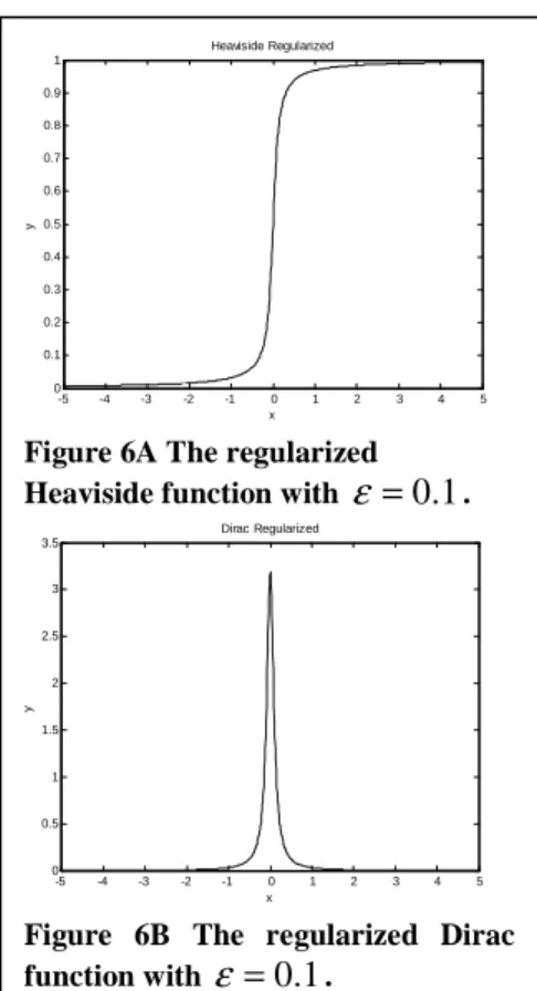
Ω ∇ = ≈L x y H x y dxdy C _ε(φ( , )) _ε(φ( , )) (12)

where H is the regularized Heaviside _ε

function: )) ) , ( ( tan 2 1 ( 2 1 lim )) , ( ( 1 0 ε φ π φ ε ε y x y x H − → + = (13)

and analogously, the regularized Dirac function can be defined by:

-5 -4 -3 -2 -1 0 1 2 3 4 5 0 0.1 0.2 0.3 0.4 0.5 0.6 0.7 0.8 0.9 1 x y Heaviside Regularized

Figure 6A The regularized Heaviside function with ε =0.1.

-5 -4 -3 -2 -1 0 1 2 3 4 5 0 0.5 1 1.5 2 2.5 3 3.5 x y Dirac Regularized

Figure 6B The regularized Dirac function with ε =0.1.

) ) , ( ( 1 lim )) , ( ( _{2 2} 0 _{x y} y x φ ε ε π φ δ ε ε = _{→ +} (14)

Following Eq.12, Eq.13 and Eq.14 we have:

      ∂ ∂ ∂ ∂ ∂ ∂ ∂ ∂ =       ∂ ∂ ∂ ∂ = ∇ x H x H y H x H y x H φ φ φ φ φ ε ε ε ε ε( ( , )) , , (15) So that,

( )

( )

( )

, ,

(

( , )

)

( , ) 1 )) , ( ( , 1 1 1 1 , 1 1 1 1 2 2 2 2 2 2 y x y x y x y x y x H y y x y H x y x x H φ φ δ φ φ φ ε ε π φ φ ε φ ε π φ φ φ ε φ ε π φ φ ε ε ε ε ∇ =       ∂ ∂ ∂ ∂ + = ∇ ∂ ∂ + = ∂ ∂ ∂ ∂ ∂ ∂ + = ∂ ∂ ∂ ∂ (16)

Substituting ∇H_ε(φ(x,y)) in Eq.12, we get

∫

Ω

∇

≈ x y x y dxdy

C δ_ε(φ( , )) φ( , ) (17)

Another function of φ(x,y) can be used to approximate the area of the contour:

∫

Ω

≈ H x y dxdy

w _ε(φ( , )) (18)

As we can observe from the Eq.17, the length of C is approximated by the sum of all the norms of the gradient of φ(x,y)=0 for each point (x, y) . The area of the contour is approximated by the sum of all points that are inside the contour.

The minimization of this length leads to the following evolution equation:

        ∇ ∇ ⋅ ∇ = ∂ ∂ φ φ φ δ φ )) , ( ( x y t (19)

In comparison with the snakes method, the main advantage of level sets method is that it handles naturally cavities, concavities, convolution, splitting or merging on contours. The initial curve can be a closed contour and evolve to two closed contours or vice versa. Due to this fact, it is possible an arbitrary initialization of the contours which excludes the need for having previous information about the objects. It also allows the segmentation of objects with discontinuous edges, that is, it can handle contours which are not regular.

2 . 7 E d g e B a s e d

For an Edge-Based approach an additional term is introduced in the snake model functional. This term depends on the gradient of the intensities. Within this approach, the boundary of an object takes place when the gradient is maximal. It estimates whether a given point in the image separates two distinct and uniform areas, assuming that this point pertains to the object’s boundary. Therefore, the stopping criterion for the minimum of energy is a gradient maximum. As follows:

∫

∫

+ − ∇ =L C s C s ds L u C s ds E 0 2 0 0 2 '' 2 ' )) ( ( ) ) ( ) ( (α β λ (20)

An Edge Based active contour model uses local properties in order to constrain the movement of the curve. As it evaluates local minimums it is very susceptible to noise.

2 . 8 R e g i o n B a s e d

A Region Based active contour model uses global properties in order to constrain the movement of the curve. These models evaluate the uniformity of regions in the image, considering that a uniform region is associated with an object and it also evaluates the smoothness as a parameter of regularity. For a Region Based model, the functional has terms that evaluate the uniformity of parameters like intensity, colour, texture, etc. The segmentation energy for region based active contour models is described by the functional of Mumford-Shah.

2 . 9 M u m f o r d - S h a h F u n c t i o n a l

The application of the Mumford-Shah functional proposes the following solution to the segmentation problem: given an observed image u , find a ₀

decomposition ω_i of ω, such that the new segmented image u then varies smoothly within each ω_i, and discontinuously across the boundaries of ω_i. The Mumford-Shah functional can be written as:

∑ ∫

− + = Ω i i o x y c dxdy C u C u E i | | ) , ( ) , (

λ

2

ν

(21)

The minimization process depends on c , which is the mean intensity in the _i

region ω_i, which is term associated with homogeneity; and depends on C characteristics, where C is a set of curves in

ω

, i. e., it is the set of boundaries of the objects.

In 2001, Chan and Veese[5] developed a new approach to active contours using the Mumford-Shah functional instead of the classical approach based on

the gradient. They also used the level set method formulation of the model. Their functional integrates the terms that evaluate the smoothness within a region and also two more terms. These terms establish constraints on the length of object’s boundary and its area. The length constraint can help eliminating isolated points near the boundaries of the objects whereas the area constraint may eliminate islands of points associated with noise. The full functional becomes. ) 0 ( ) 0 ( ) , ( ) , ( ) , ), , , ( ( ) ( 2 2 ) ( 2 1 2 1 = ⋅ + < ⋅ + + − + − =

_∫

_∫

φ ν φ µ λ λ φ φ φ Length Area dxdy c y x u dxdy c y x u c c t y x E outside o inside o (22)

Now that all these concepts were introduced we can discuss how this segmentation method can be implemented and what kind of results can be obtained.

2 . 1 0 D i s c r e t e a n a l y s i s

First we need to define the functional E (Eq. 22) in the discrete space:

) 0 ( )) , , ( ( ) , ( ))) , , ( ( 1 ( ) , ( )) , , ( ( ) , ), , , ( ( , , 2 2 0 , 2 1 0 2 1 = ⋅ + + + − − + + − =

∑

∑

∑

φ ν φ µ φ λ φ λ φ Length t j i H c j i u t j i H c j i u t j i H c c t j i E j i j i j i (23)

where H (φ ) is the Heaviside function:

   < ≥ = 0 , 0 0 , 1 ) ( φ φ φ H (24)

and

δ

(

φ

)

is the derivative of H (φ ) , i. e., the Dirac function:

   ≠ = = 0 , 0 0 , 1 ) ( φ φ φ δ (25)

As we are working in a discrete level φ (i, j,t) is only rarely equal to zero. Therefore, for a discrete level we must work with the regularized versions of

) (φ

H and δ (φ ) (Eq. 13 and Eq.14). To determine the length of the contour we define an auxiliary function, γ(φ(i,j)), that evaluates if a pixel is a boundary point. γ(φ(i,j)) was defined by De Santis and Iacoviello[7] as:

[

1 ( ( (, )))

]

))) , ( ( 3 ( )) , ( (φ i j H ρ φ i j δ ρ φ i j γ = − − (26)

and ρ(z(i, j))is defined as:

[

]

∑

− − + + − + = 1 1 2 2 ))) , ( ( )) , ( ( ( ))) , ( ( )) , ( ( ( )) , ( (z i j H z i l j H z i j H z i j l H z i j ρ (27)

The function ρ(φ(i,j)) evaluates how many times the signal of )

, ,

(i j t

φ

changes within the close neighbours of a particular pixel (see Fig.7). In such way that:

• if ρ(φ(i, j))=3, then one of the neighbours has the same signal for ) , , (i j t φ as the pixel ) , (i j . Hence, (i, j) belongs to the boundary. • if ρ(φ(i, j))=2, then two

of the neighbours have the

same signal for

) , , (i j t

φ

as the pixel ) , (i j . Hence, (i, j) belongs to the boundary. • if ρ(φ(i, j))=1, then three

of the neighbours have the

same signal for

)

,

,

(

i

j

t

φ

as the pixel ) , (i j . Hence, (i, j) is a boundary pixel. • if ρ(φ(i,j))=4, then all

four neighbours have the same signal for

φ

(

i

,

j

,

t

)

among them, but different signal from the pixel (i, j) . Hence, (i, j) is an isolated pixel. • if ρ(φ(i,j))=0, then all five pixels have the same signal for

φ

(

i

,

j

,

t

)

.

Hence, (i, j) is an interior pixel.

Observing the functionγ(φ(i,j)), we can see that:

• if ρ(φ(i, j))=4 thenH(3−ρ(φ(i,j)))=0 otherwise H(3−ρ(φ(i, j)))=1; • if ρ(φ(i, j))=0 then

[

1−δ(ρ(φ(i,j)))

]

=0 otherwise

[

1−δ(ρ(φ(i, j)))

]

=1; In conclusion, we will use γ(φ(i,j))to count the number of pixels that belong to the boundary so that we can determine the length of the curve C .

In this way we can define the energy as:

∑

∑

∑

∑

+

+

+

−

−

+

−

=

j i j i j i j i

t

j

i

t

j

i

H

c

j

i

u

t

j

i

H

c

j

i

u

t

j

i

H

c

c

t

j

i

E

, , , 2 2 0 , 2 1 0 2 1

))

,

,

(

(

))

,

,

(

(

)

,

(

)))

,

,

(

(

1

(

)

,

(

))

,

,

(

(

)

,

),

,

,

(

(

φ

γ

ν

φ

µ

φ

λ

φ

λ

φ

(28) Figure 7 The function ρ(φ(i,j)) assesses the signal change of the function φ(i, j)for the neighbours of

The algorithm of the method can be divided in the following steps:

• the method initializes with an arbitrary field φ(x,y) defining an arbitrary curve, φ(x,y)=0;

• the arbitrary curve defines two domains (inside and outside) depending on the sign of φ(x,y);

• the mean intensity inside each domain, c and ₁ c , is recursively ₂

calculated so that the functional in Eq. 28 is minimized;

• given these values of c₁ and c₂, equation 28 is calculated and a recurrent equation is used to minimize E(φ(i, j,t),c₁,c₂) relatively to variations in

) , (x y

φ . This changes φ(x,y,t) so that the curve defined by φ(x,y)=0 tends to fit the segmented region.

De Santis and Iacoviello[7] also introduced a term in the functional that forces the convexity of the function E , so that φ(x,y,t) never diverges. The full functional then becomes:

∑

∑

∑

∑

∑

+ + + + − − + + − = j i j i j i j i j i t j i t j i t j i H c j i u t j i H c j i u t j i H c c t j i E , 2 , , , 2 2 0 , 2 1 0 2 1 ) , , ( 2 )) , , ( ( )) , , ( ( ) , ( ))) , , ( ( 1 ( ) , ( )) , , ( ( ) , ), , , ( (

φ

α

φ

γ

ν

φ

µ

φ

λ

φ

λ

φ

(29)

The framework that we are using considers that the partition of the image in regions can be determined by an energy minimization which leads to:

            = ∂ ∂ = ∂ ∂ = − − = ∂ − ∂ = ∂ ∂

∑

_∑

_∑

0 0 0 ) )) , ( ( ) , ( )) , ( ( ( 2 ) , ( )) , ( ( ( 2 , 1 0 , 1 , 2 1 0 1 φ φ φ λ φ λ E c E j i H c j i u j i H c c j i u j i H c E j i j i j i (30)

The minimization involves two steps. From the first two equations in Eq. 30, we obtain:

∑

∑

= j i j i j i H j i u j i H c , , 0 1 )) , ( ( ) , ( )) , ( ( φ φ (31)

and

∑

∑

− − = j i j i j i H j i u j i H c , , 0 2 ))) , ( ( 1 ( ) , ( ))) , ( ( 1 ( φ φ (32)

The constants c and₁ c are mean of intensities of the domain 1 (₂ φ>0) and domain 2 (φ<0), respectively. Then the partial derivative of the E in relation to φ leads to:

(

)

(

(

)

)

(

)

0 ) , ( 2 )) , ( ( ) , ( ) , ( 1 ) , ( , 2 , , 2 2 0 , 2 1 0 , =       ∂ ∂ +       ∂ ∂ + +       ∂ ∂ + +       − − ∂ ∂ +       − ∂ ∂ = ∂ ∂

∑

∑

∑

∑

∑

j i j i j i j i j i j i j i j i H c u j i H c u j i H E φ φ α φ γ φ φ φ µ φ φ λ φ φ λ φ (33) which becomes:

(

)

(

)

0 ) , ( 2 2 )) , ( ( )) , ( ( )) , ( ( )) , ( ( , 2 2 0 2 1 0 = +         ∂ ∂ + + + − − − = ∂ ∂

∑

i j i j j i j i c u j i c u E j i

φ

α

φ

γ

φ

ν

φ

µδ

φ

δ

λ

φ

δ

λ

φ

(34) where,

0

))

,

(

(

,

=

∂

∂

∂

∂

∂

∂

=

















∂

∂

_∑

φ

ρ

ρ

γ

γ

φ

γ

φ

E

j

i

j i (35) so that,

(

) (

)

(

)

[

]

( (, )) 0 1 ) , ( ₀ 22 2 1 0 =            ∂ ∂ ∂ ∂ ∂ ∂ + + − − − + φ ρ ρ γ γ ν φ δ µ λ α φ i j u c u c i j E (36) Finally,

(

)

(

) (

)

[

( ( , )) ( (, )) ( (, )) ( (, ))

]

) , , ( 0 ) , ( ) , ( ) , ( ) , , ( ) , ( 1 1 j i H l j i H j i H j l i H l j i r j i j i j i q l j i r j i p l

φ

φ

φ

φ

αφ

φ

δ

ν

µ

λ

− + + − + = = +       + +

_∑

− = (37)

where p( ji, ) stands for:

(

) (

)

2 2 0 2 1 0(, ) (, ) ) , (i j u i j c u i j c p = − − − (38) ) , ( ji q stands for:

(

)

[

]

)) , ( ( )) , ( ( 2 ) , ( )) , ( ( ) , ( ))) , ( ( 3 ( )))) , ( ( ( 1 ( ))) , ( ( 3 ( 2 ) , ( 2 2 j i j i j i s j i j i s j i H j i j i j i q φ ρ ε φ ρ φ ρ δ φ ρ φ ρ δ φ ρ δ + = − − − ⋅ − = (39)

Thus, the energy minimization has been transformed in the problem of finding the zeros of a function defined in a multidimensional space. A straightforward way of solving this problem is to use a fixed point method to find the recurrent equations. Having an equation of the type G(φ(i,j))=0, we rewrite it as

) , ( ) , ( )) , ( ( i j i j i j

Gφ +φ =φ which can be solved using the iterative method of searching for the fixed point (see Fig.8), which corresponds for the zero of the function.

2 . 1 1 F i x e d p o i n t i t e r a t i o n m e t h o d

If we consider φ₀ as an initial function, corresponding to initial arbitrary contour curves for which G(φ(i,j))=0, we can write the recursive fixed point equation: ) ( 1 n n n kGφ φ φ + = ± _{,n=0,1,..N (} 40) Here φn

is the field of iteration n, k a constant whose sign and magnitude should be chosen so that the recursive equation converges to the fixed point, for which φn+1₌φn_{, and}

hence G(φn)=0. Determining

n

n φ

φ +1 =

solves the minimization problem. In this case, Eq.40 should be iterated until φn+1 φn 1+ −φn_〈ε

, where εis a tolerance limit fixed a priori. Hence, the recursive relation is defined as

Figure 8 An example of the application of the fixed point iteration method

(

)

_                   + + + ± =

_∑

− = + ) , ( ) , , ( ) , ( ) , ( 1 ) , ( ) , ( ) , ( 1 1 1 j i l j i r j i q j i p j i k j i j i n l n n n n n λ µ ν δφ α φ φ φ (41)

The constant k should be chosen so that the method converges and quickly. Here was used k =−0.5. This method has a high cost on computational time because φ is updated for each pixel per iteration. For a matrix with 200x200 pixels this means that for 4 iterations 160000 updates are required. If per iteration are required 2ms of computational time, then a segmentation process could require 32 seconds, only for one image.

2 . 1 2 T h e a p p l i c a t i o n o f t h e s e g m e n t a t i o n m e t h o d

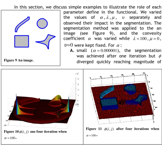
In this section, we discuss simple examples to illustrate the role of each parameter define in the functional. We varied the values of

α

,λ,µ,

υ

separately and observed their impact in the segmentation. The segmentation method was applied to the an image (see Figure 9), and the convexity coefficient

α

was varied while λ =100,µ=0,

0

=

υ

were kept fixed. For α:

A. small (α =0.000001), the segmentation was achieved after one iteration but

φ

diverged quickly reaching magnitude of

the order of 11

10 (see Fig.10);

B. large (α =100) four iterations were required and the magnitude of φ remained finite, of the order of 1

10 (see Fig.11). If we compare the surface φ for both situations A and B:

Figure 9 An image.

Figure 10φ( ji, ) one four iteration when

100

= α .

Figure 11 φ( ji, ) after four iterations when

100

=

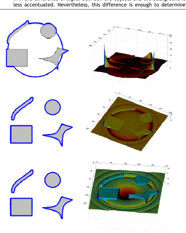
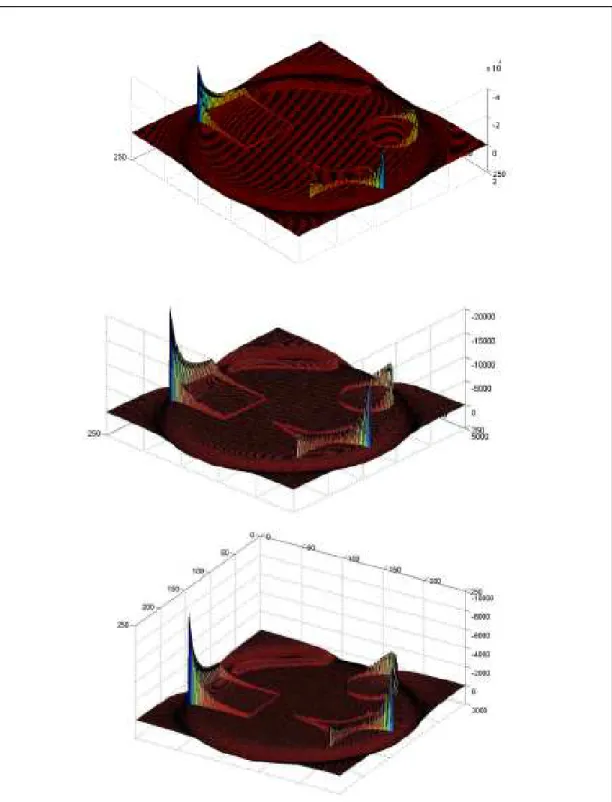
• in A the difference of signal between the objects and the background is less accentuated. Nevertheless, this difference is enough to determine

the boundaries of the objects;

• it can also be observed in situation A, that inside the objects there are different values for _φ;

Figure 10 This sequence of images shows: on the left the segmentation of the image and on the right the corresponding surface φ for the application of the method with λ =1. As we could observe, the segmentation of image is achieved in the second iteration. Despite of this, the part of the surface φ corresponding to objects only achieved an expressive difference from the background in the third iteration.

Figure 13 This sequence of images shows the surfaces of φ using λ =100. The segmentation of the image was achieved in the first iteration (first image) but it was not achieved the convergence of φ as the surfaces of the 2nd and 11th iterations show.

• in B φ has a different signal for the objects and the background. • there is also an accentuated difference in the magnitude of φ for both situations, of order of 1011 for situation A and 100 for situation B.

Figure 14 Application of the method using different values for coefficient µ

Therefore, with this example we understand that the parameter

α

can be

useful to avoid computational

divergences.

Next, we used two different values for coefficient associated with homogeneity, λ =1 (see Fig. 12) and

100 =

λ (see Fig. 13), while

100 =

α ,µ=0, υ=0(see). Further, when 0

=

λ the segmentation is not achieved. This is predictable as this is the main term of the method associated with homogeneity. For cases like the one in Figure 9 this parameter and the one associated to convexity are enough to make this segmentation method to work properly.

In the next examples were used three values for the coefficient associated with the area µ= −100,

10 − = µ and µ=100 while λ =0.01, 1 =

α , υ=0 where kept fixed (see Fig. 14). In case A there is a competition between both circles. Nevertheless, the black circle is the one that has the larger difference from the background’s intensity. Although, λ has a low value it is the most important term in the segmentation so there is a balance between both parameters. In case B the segmentation for both circles was obtained. The value of µ is still negative but not too low so that the area must not be so small that it forces the exclusion of the grey circle. The last case, C, shows the maximization of the area for the parameter with positive signal. The segmentation was not successful. In the next examples we varied the value of the coefficient associated

with the minimization of the contour length , ν = −1000,ν =10 and ν =100 while λ =0.01, α =1, µ =0 where kept fixed (see Fig.15). As can be observed the parameter minimizes the length if it is positive. Figure 15D shows that if the parameter ν is considerably negative it will introduce an error that does not disappear. In Figure15E, the segmentation was successful for both circles and the same happens in Figure15F, in spite of the ν increase. On the contrary, in G the grey circle is not segmented. The grey circle has a value of intensity closer

to black values to white. So the strength of ν is not enough to exclude the grey circle and minimize the length. Hence in case G the light grey was not detected. This situation was reverted by giving more strength to the difference of intensity of the grey circle in relation to the background that is, increasing λ =10 (situation H).

We conclude that a balance between parameters α,λ,µ, υ must exist. Summarizing: • the parame ter λ is the most importa nt in the energy function al; • the parame ter α is

necessary for the convexity of the of energy function; • the parameter µ must be a negative, to minimize the area; • the parameter υ must be positive, to minimize the length;

Figure 11 Application of the method using different values for coefficient ν.

Figure 16 The application of the method with the parameters 01

. 0 =

α ,λ =1,µ=−100,ν =100 to images U and V. The image U and the image V are equal, excluding the colour of the points that simulate noise.

Neve rtheless, all the parameters should be defined after a careful observation of the images to which the method is to be applied. For instance, • if the imag e show s a high cont

rast between the background

and the objects, the

homogeneity term does not have to be very strong (small values for λ).

• if there is a low contrast

between objects the

homogeneity term has to be strong (λ big);

• if the boundaries of the objects are regular, the

terms associated with

regularity must no be very strong (µ, ). ν

• if the image has noise the regularity terms should be

strong (positive values for ν and negative values for µ); and what kind of noise (e.g. for isolated points, the term associated with the length minimization ν should be strong and for islands the term associated with the area minimization µ should be strong)

Figure 17 The application of the method to typical images, using different values for the parameters λα,λ,µ,ν .

0 50 100 150 200 250 0 500 1000 1500 2000 2500 intensity fr e q u e n c y

Figure 18 The histogram of intensities corresponding to the image in Figure 20X.

Bearing these aspects in mind, we present next some examples for which the method either is successful or fails. In the first case in Figure 16 the segmentation was successful in spite of the ‘noise’ from light grey dots. However, in the second case where the ‘noise’ has the same colour as the object, and consequently the segmentation fails.

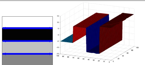
In Figure 17A, the segmentation was successful. In the image were detected four objects. We can see in the surface φ the fourth changes of signal between adjacent areas. In this case, the colours were interlaced by values of intensity. However, in the image in the Figure 17B, the segmentation fails. In this image only two objects were detected: the darker part of the image (black and dark grey) and the lighter part (white and light grey). Although the surface φ could be divided in four different areas, the change of signal is between the area that has a high mean of intensity and the area that has a low mean of intensity. Even with an increase of the parameter λ, which gives more strength to the

Figure 19A) On the left is the image used and the resulting segmentation. On the right is represented the surface φ. The parameters used were α =10,λ =10,µ =0,ν =0

Figure 19B) On the left is the image used and the resulting segmentation. On the right is represented the surface φ The parameters used were α =10,λ =10,µ=0,ν =0

difference between the intensities of the different areas, we had was no success in performing a good segmentation.

The last example will be present in the typical eye images that were obtained. The object that we want to isolate from the rest of the image is the pupil. In order to increase contrast between the pupil and the iris, a infra red lamp is used. The pupil absorbs the infra red light so that it is, in principle, the darker object in the image. As we can observe for the different cases in Figure 18, the segmentation failed. In Figure 19 is represented the histogram of intensities of a typical image. For determining the centre of the CR it was applied a simple threshold on the image. As we can see there is a peak associated with the intensities above 250. In the case of the pupil the threshold does not work since there are several pixels with the same intensity has the pupil.

In order to improve the segmentation,

we included the condition c₁=0 where c₁ is the mean of intensity of the domain 1, only for the first iteration of the segmentation method. In spite the first iteration showed better results, the surface φ evolved to the same kind of surface previously in the images of Figure 18. As the result obtained in Figure 20A was closer to a good solution, we tried to develop a complementary method which used that information to determine the center of the pupil. This method also finds an energy extremum based on energy minimization and it will be presented in section 2.14.

2 . 1 3 I m a g e s e g m e n t a t i o n a p p l i e d t o o p t i c a l i l l u s i o n s The previous

problems found in the application of the active contours method can be best illustrated when it is applied to optical illusions. The study of optical illusions from a scientific point of view has increased recently,

since they allow a simple analysis of how our brain functions. In connection to segmentation problems it is really an interesting approach since it is known that

Figure 20 In A is represented the application of the method to typical images constraining the value of c₁

in the first iteration. In B is represented the method after thirteen iterations.

Figure 21 Although the central patch is exactly the same in all cases, simultaneous brightness contrast makes it appear to vary from dark to light as the background is changed from light to dark.

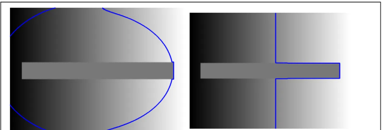
our brain outperforms current computational algorithms when performing the same tasks. Thereafter, we choose one optical illusion in particular and analyse how the active contours performs the segmentation task. The optical illusion used is an example of a gradient illusion (see Fig.22). All the pixels in the central bar have the same intensity. This can be checked if the background is removed, isolating the bar. However, we perceive a bar with a gradient of intensity. The illusion results from the background gradient effect on the process of defining the reflectance of the object to which we are looking at (which in this case is the bar).

Our perceptual system has the ability to adjust to different light conditions, that is, it sees objects as continuing to have the same brightness even though light may change their immediate sensory properties. An object will exhibit brightness constancy as long as both the object and its surroundings are in light of the same intensity. If the background brightness differs from the object, brightness constancy is not maintained. For instance, a sheet of white paper seen in the bright sunlight reflects a very different amount of light than the same sheet of paper seen later that night in a softly lighted room. Yet we perceive the paper as having the same whiteness in each case. The gradient illusion breaks brightness constancy.

In Figure 22 we can observe that the segmentation method was not successful. This method uses the global properties of the image in order to achieve the energy minimization. If we consider a symmetrical division of the image along the y axis, the intensity mean for each domain is equal so that it is not possible to define different domains. In the case of Figure 21 (on the right) were defined two domains due to a break of symmetry. By repeating application of the method, it should be obtained, for half of the times, the result in Figure 21 (on the right) and the symmetric result (the left part of the bar) for the other half of the times.

2 . 1 4 M e t h o d t o d e t e r m i n e t h e p u p i l c e n t r e o f m a s s

As we mentioned in the end of section 2.12, we used the information given by the segmentation method and developed a new and simple algorithm to locate the coordinates of the pupil centre. In spite of this approach, we did not

Figure 22 The segmentation of the gradient optical illusion. The image on the left shows the first iteration and the image on the right shows the sixth iteration.

achieve the desired robustness, as it will be discussed. Overall, we established a new method to determine the pupil centre which does not uses the active contour approach.

We will first present a simple 1D example in order to explain clearly what it the framework of our method. Consider two functions f(x) and

G

(x

)

, where

)

(x

G

is a Gaussian function centred around an arbitrary position,

X

, and

f

(x

)

is a square well (for the sake of simplicity) (see Fig.23):

(

)

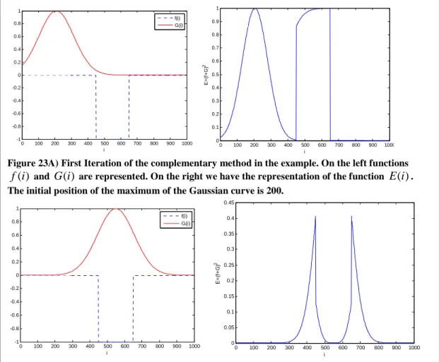
) 2 exp( ) ( , 0 , , 0 ) ( ₂ 2 4 3 3 2 1 0 σ X x x G x x x x x x X x x x x f = − −      ≤ 〈 ≤ 〈 ≤ ≤ = (42)

We want to find the coordinates around which the Gaussian should be centred so that the two functions have maximal overlap, i.e., their sum is minimum (see Fig.23). Hence we define an energy function given byE

( ) (

x w x

)

dx

x x

∫

= 4 0 2 ) ( where ) ( ) (x Gx f

w= + , and (see Fig.23). The minimum of E is achieved when:

(

( ) ( )

)

( ) ( ) 0 2 ) ( ) ( 0 )) ( ) ( ( 2 0 ) ( 2 0 2 2  =    − + =     ₋ − + = ⇔ =       ∂ ∂ ∂ ∂ + ∂ ∂ ∂ ∂ = ⇔ = ∂ ∂ ∂ ∂ = x G X x x G x f x G X x x G x f dx dE x G G w x f f w x w dx dE x w w E dx dE σ σ (43)

A discretization of these equations leads to:

(

() ()

)

( ) () 0 2 2 =    − +

∑

i i G I i i G i f σ (44)

Thereafter, the minimum can be calculated iteratively using the fixed point iteration method, as we did in Eq.31:

) ( 1 n n n _{I kT I} I + = ± (45) where:

(

)

∑

      ₋ − = i n n i G I i i G i f I T( ) () () ( ₂ ) () σ (46)

n

i is the value of i on the ith iteration and k is a constant that accelerates or decelerates the convergence. In this case we used k =0.001.

In this way the position of the maximum of the Gaussian curve moves along the time and the convergence is achieved when the overlapping is maximal

0 100 200 300 400 500 600 700 800 900 1000 -1 -0.8 -0.6 -0.4 -0.2 0 0.2 0.4 0.6 0.8 1 i f(i) G(i) 0 100 200 300 400 500 600 700 800 900 1000 0 0.1 0.2 0.3 0.4 0.5 0.6 0.7 0.8 0.9 1 E = (f + G ) 2 i

Figure 23A) First Iteration of the complementary method in the example. On the left functions )

(i

f and G(i) are represented. On the right we have the representation of the function E(i). The initial position of the maximum of the Gaussian curve is 200.

0 100 200 300 400 500 600 700 800 900 1000 -1 -0.8 -0.6 -0.4 -0.2 0 0.2 0.4 0.6 0.8 1 i f(i) G(i) 0 100 200 300 400 500 600 700 800 900 1000 0 0.05 0.1 0.15 0.2 0.25 0.3 0.35 0.4 0.45 i E = (f + G ) 2

Figure 23B) Last iteration of the method (22). As we can see the Gaussian moved so that the minimum of (f(i)+G(i))2 is achieved when the centre of the Gaussian is at i=550.

Figure 12C) On the left we can see the projection on planes x and y of the surface associated to a typical eye image obtained. On the right we can see the surface of pixel intensities. There are similarities between this surface and the f(i) function from the previous example.

(minimum of E(i) is achieved)) is achieved. An example can be observed in Figure 23A, B, C. Although this is a simple method, it is interesting to show it works. In the Figure 24 the determinat ion of the centre of mass of a circle is shown. The Gaussian surface has a 40 = σ pixe ls so that σ 2 is larger than the circle radius which equals 60 pixels. Images D, F and H show

(

)

2 20 G I+ ⋅ where I is the image surface and G is the Gaussian

has a factor of 20 so that its possible to observe the Gaussian maximum in the figure . For calculations this factor was not considered.

In eyes’ images, there is more than one dark object (see Fig.20A). Hence, the method was also applied to more complex examples, similar to the example in Figure 20A. What was observed was that the Gaussian surface would not always be centred in the centre of mass of the pupil depending on:

• the initial coordinates of the centre of the Gaussian; • the sigma of the Gaussian surface;

Figure 25 shows some typical examples.

If we look to the Figures25M and 25P, we can see that the intermediate positions are close to the centre of mass of the circle. In spite of this the

method does not converge to the centre. The value of sigma is too large (larger than the radius of the circle) the second object competes strongly by the position of minimum. We can conclude that the centre of mass of the circle was not determined correctly. This happened because the value of sigma was too large allowing the second object to contribute largely to the minimum of energy.

Figure 25 In this example we can observe that different initial points can have different convergence points.

In Figure 27 are shown the examples of the results of the application of the method, using the initial points previously considered (see Fig.25), but a smaller sigma, σ =20. In Figure 26R the minimum converged to a position inside the second object. The contribution of the circle decreased so that the major contributions were from the second object. In Figure 26S, the maximum was not achieved because there were no contributions from both objects as the sigma was insufficiently large. In Figure 26T, we can see that the method converged to the desired position. This was a result of a compromise between the initial point which was sufficiently close to the circle and sufficiently far from the second object. In this case σ that was not sufficiently large to consider the contributions from the second object.

Since the method was not robust as it depended on the initial conditions, it was necessary to have an estimation of the centre of mass of the pupil, so that the initial conditions could be wisely chosen. After the application of the active contour without edges, we defined a way of guaranteeing the compromise between the parameters involved in the complementary method: the value of sigma and the position of the initial point. In order to choose an appropriate initial point for the fixed iteration point method, we defined that this point should be the centre of mass of the corneal reflection. We also defined a region of interest in the image in order exclude the possibility of competition between dark objects. Furthermore, as the number of elements in the matrix decreased, the computational time improved considerably. We think this method is more robust than the active contours without edges for the case of our images.

Figure 26 The final positions associated with a sigma equal to 20.

In Figure 27 we can observe the application of the method. The initial point of start for the method is the corneal reflection centre of mass (white spot). Using this point and the value of sigma, a region of interest is defined. As there is a relation between the position of corneal reflection and the position of the pupil, the problems associated with fast variations of the position of the pupil are minimized. In Figure 27A is represented the position achieved in the second iteration. In Figure 27B is represented the final position achieved with the method after 21 iterations. This corresponded to a computational time equal to 0.841 seconds. As we can see the shape of the pupil has not eccentricity exactly equal to the eccentricity of a circle. This means that using the Gaussian to determine the pupil centre is an approximation. In order to minimize

the error associated to this

approximation, we considered an additional procedure. When the

convergence is achieved

(In+1−In <0.001), the value of n+1

I is disturbed for a small value (see Table 1) and the method is applied again. However the precision of the eye tracker is not affected. For tasks which goal is not to determine its accurate position but to assess the variation of the movements of the eye, this aspect of the method is not determinant.

Figure 27 In A are represented the coordinates obtained by the method in the second iteration, inside the region of interest (97pixelsx123 pixels). In B is a graph that shows the centre of mass obtained by the method (yellow dot) after 21 iterations. This graph was obtained using the MATLAB instruction colormap (lines);pcolor(I). The colours are associated with intensity values. This representation was used in order to show a typical shape obtained for the pupil. In C it is represented the position of the pupil centre obtained. The image had a 200pixelsx200pixels resolution so using the region of interest represents a reduction of 70% in the size of the matrix.

Table 1 Typical results after achieving the

point of convergence. We summed

disturbances along x and y and performed the method again. The results gave variations of the order of the 0.001. Hence, this not solve the problem associated with the eccentricity of the pupil

3 . N

E U R A L

N

E T W O R K S

3 . 1 I n t r o d u c t i o n

Neural Networks are a mathematical framework that aims to reproduce the same type of intelligent behaviour as that displayed by humans. Its architecture was inspired in the human brain, and consequently their constituents are also called neurons and their interactions are called synapses. These serve to receive and send information. The information that reaches a neuron can arrive from different synapses. These can have different impact on the neural response. Hence, each neuron can integrate signals coming from different channels simultaneously, and also send information to several neurons at the same time. The importance of each connection depends on the training that is given to the brain. For instance, while we are children we train for a long time how to grab an object properly. That process of trial and error influences the way connections are established between neurons. As a result, the brain gains the ability to:

• Recognize patterns in the presence of noise; • Recall memories;

• Make decisions for current problems based on prior experience;

As can be observed in Figure28, Neural Networks intend to reproduce these capabilities in a more basic way. The biological model of the neuron also receives information, activating the neuron and producing an output. Also, each neuron is connected to other neurons (synapses).

There are many different types of neural networks depending on the task they are planned for. Each type of neural network is specified by a neuron model, a network architecture and a learning algorithm. The neuron model is defined by a response function which establishes how an output corresponds to a certain input, that is, activates the neuron. The architecture establishes the number of neurons that compose the network. The learning algorithm defines the process through which the network increases the intensity of certain interactions (i.e., their weights) and not others. This is essential to establish the correct association between inputs and outputs. The input information and the connection (synaptic) weights are the arguments of the

Figure 28A) The biological model of a neuron.

Figure 28B) The mathematical model for a neuron. Neurodes in an Artificial Neural Network receive signals from other neurodes or from external sources, perform transformations on them, and then pass those signals on to other neurodes.