CERN-EP-2018-167 2018/07/03
CMS-SMP-16-003
Measurement of differential cross sections for inclusive
isolated-photon and photon+jets production in
proton-proton collisions at
√
s
=
13 TeV
The CMS Collaboration
∗Abstract
Measurements of inclusive isolated-photon and photon+jets production in proton-proton collisions at√s =13 TeV are presented. The analysis uses data collected by the CMS experiment in 2015, corresponding to an integrated luminosity of 2.26 fb−1. The cross section for inclusive isolated-photon production is measured as a function of the photon transverse energy, for ET > 190 GeV, and rapidity, for|y| <2.5. The cross
section for photon+jets production is measured as a function of the photon transverse energy, for ET >190 GeV, the photon rapidity, for|y| <2.5, and the rapidity of the jet
with highest transverse momentum, up to|y| <2.4. The experimental measurements are found to be in agreement with predictions from perturbative QCD.
Submitted to the European Physical Journal C
c
2018 CERN for the benefit of the CMS Collaboration. CC-BY-4.0 license
∗See Appendix A for the list of collaboration members
1
Introduction
The measurement of inclusive isolated-photon and photon+jets production cross sections can directly probe quantum chromodynamics (QCD). The dominant production processes in proton-proton (pp) collisions at the energies of the CERN LHC are quark-gluon Compton scattering qg→qγ, together with contributions from quark-antiquark annihilation qq→gγ, and parton fragmentation qq(gg) →X+γ. Both the CMS and ATLAS Collaborations have reported mea-surements of the differential cross sections for isolated prompt photon production [1–5] and for the production of a photon in association with jets [6–8] using data with center-of-mass ener-gies of 2.76, 7, and 8 TeV. The ATLAS Collaboration has also reported the same measurements at a center-of-mass energy of 13 TeV [9, 10].
The published measurements show agreement with the results of next-to-leading-order (NLO) perturbative QCD calculations [11, 12]. Although these LHC measurements are not currently included in the global parton distribution functions (PDF) fits [13–15], they are sensitive, in par-ticular to the gluon density function g(x, Q2)over a wide range of parton momentum fraction x and energy scale Q2 [16–18]. An improved understanding of all PDFs is key to reducing the
associated theoretical uncertainties in the calculation of many relevant cross sections, including Higgs boson production and new physics searches.
In this paper, measurements of the inclusive isolated-photon and the photon+jets production cross sections are reported using data collected by the CMS Collaboration in 2015 during 13 TeV proton-proton collisions, corresponding to an integrated luminosity of 2.26 fb−1 [19]. The sig-nificant increase of center-of-mass energy, compared to the previous CMS measurements [1, 2], opens a large additional region of phase space.
The dominant background for the photon+jets process is QCD multijet production with an iso-lated electromagnetic (EM) deposit from decays of neutral hadrons, mostly from π0mesons. A
multivariate analysis method is used to identify prompt photons using a boosted decision tree (BDT) algorithm, implemented using the TMVA v4.1.2 toolkit [20]. Photon yields are extracted using the shape of the BDT distributions, and the measured cross sections are compared to the results of NLO QCD calculations.
2
The CMS detector
CMS is a general-purpose detector built to explore physics at the TeV scale. The central fea-ture of the CMS apparatus is a superconducting solenoid of 6 m internal diameter, providing a magnetic field of 3.8 T. Within the solenoid volume are a silicon pixel and a strip tracker, a lead tungstate crystal electromagnetic calorimeter (ECAL), and a brass and scintillator hadron cal-orimeter (HCAL), each composed of a barrel and two endcap sections. Forward calcal-orimeters extend the pseudorapidity η coverage provided by the barrel and endcap detectors. Muons are measured in gas-ionization detectors embedded in the steel flux return yoke outside the solenoid. A more detailed description of the CMS detector, together with the definition of the coordinate system and the relevant kinematic variables, is given in Ref. [21].
The ECAL consists of 75 848 lead tungstate crystals, which provide coverage up to|η| =1.479 in the barrel region (EB) and 1.479< |η| <3.0 in two endcap regions (EE). A preshower detec-tor consisting of two planes of silicon sensors interleaved with a total of 3 radiation lengths of lead is located in front of the EE.
The silicon tracker measures charged particles within the range|η| <2.5. For nonisolated par-ticles of transverse momenta 1< pT <10 GeV and|η| <1.4, the track resolutions are typically
1.5% in pTand 25–90 (45–150) µm in the transverse (longitudinal) impact parameter [22].
The global event reconstruction (also called particle-flow event reconstruction) [23] reconstructs and identifies each particle candidate with an optimized combination of all subdetector infor-mation.
Photons are identified as energy clusters in the ECAL that are not consistent with an electron track in the tracker. The clustering algorithm allows an almost complete collection of the en-ergy of the photons, even for those converting in the material upstream of the calorimeter. First, cluster “seeds” are identified as local energy maxima above a given threshold. Second, clusters are grown from the seeds by aggregating crystals with at least one side in common with a clus-tered crystal and with an energy in excess of a given threshold. This threshold represents about two standard deviations of the electronic noise, which has an|η|dependence in the ECAL. The energy in an individual crystal can be shared between clusters under the assumption that each seed corresponds to a single EM particle. Finally, clusters are merged into “superclusters”, to allow good energy containment, accounting for geometrical variations of the detector along η, and optimizing robustness against additional pp collisions in the same or adjacent bunch cross-ings (pileup). The clustering excludes 1.44 < |η| < 1.56, which corresponds to the transition region between the EB and EE. The fiducial region terminates at |η| = 2.5 where the tracker coverage ends.
The energy of photons is computed from the sum of the energy of the clustered crystals, cal-ibrated and corrected for degradation in the crystal response over time [24]. The preshower energy is added to that of the superclusters in the region covered by this detector. To optimize the resolution, the photon energy is corrected using a multivariate technique for the contain-ment of the electromagnetic shower in the superclusters and the energy losses from converted photons [25]. In the EB, an energy resolution of about 1% is achieved for unconverted photons in the tens of GeV energy range. The remaining EB photons have a resolution of about 1.3% up to |η| = 1.0, rising to about 2.5% at |η| = 1.4. In the EE, the resolution of unconverted or late-converting photons is about 2.5%, while the remaining EE photons have a resolution between 3 and 4%.
Electrons are identified as a primary charged track consistent with potentially multiple ECAL energy clusters from both the electron and from potential bremsstrahlung photons produced in the tracker material. Muons are identified as a track in the central tracker consistent with either a track or several hits in the muon system, associated with a minimum ionization signature in the calorimeters. Charged hadrons are charged-particle tracks not identified as electrons or muons. Finally, neutral hadrons are identified as HCAL energy clusters not linked to any charged-hadron track, or as ECAL and HCAL energy excesses with respect to the expected charged-hadron energy deposit.
Jets are clustered from all particle candidates reconstructed by the global event reconstruction with the infrared- and collinear- safe anti-kTalgorithm [26, 27] using a distance parameter R of
0.4. Jet energy corrections are derived from simulation, and are confirmed with in situ measure-ments exploiting the energy balance of dijet or photon+jet events [28]. The jet energy resolution amounts typically to 15 (8)% at 10 (100) GeV.
3
Simulation samples
Simulated event samples for photon+jets and multijet final states are generated at leading or-der (LO) with PYTHIA 8 (v8.212) [29]. The photon+jets sample contains direct photon
pro-duction originating from quark-gluon Compton scattering and quark-antiquark annihilation. A filter is used to reject generated events that do not contain an isolated-photon, where the isolation requires that the sum of the pT of all stable particles within a cone of size ∆R =
√
(∆φ)2+ (∆η)2=0.4 around the photon direction is less than 5 GeV. For the multijet sample,
final states with quark and gluon jets dominate, and the photon+jets processes are explicitly removed. The MADGRAPH(v5.2.2.2) [30, 31] LO generator, interfaced withPYTHIA8, is used to generate an additional sample of photon+jet events containing up to 4 jets that is used to estimate systematic uncertainties. Samples of Z/γ∗+jets events are generated at NLO with MADGRAPH5 aMC@NLO(v5.2.2.2) [30, 32] and are used for calibration and validation studies
described later. The CUETP8M1 tune [33] is used inPYTHIA 8. The NNPDF2.3 LO PDF [34]
and the NNPDF3.0 NLO PDF [13] are used to generate simulation samples, where the former is used withPYTHIA8.
The simulated processes include the effect of pileup. The pileup contribution is simulated with additional minimum bias events superimposed on the primary event using the measured distribution of the number of reconstructed interaction vertices, an average of 14 vertices per bunch crossing. A detailed detector simulation based on the GEANT4 (v9.4p03) [35] package is applied to all the generated signal and background samples.
4
Data samples and event selection criteria
Events containing high energy photon candidates are selected using the two-level CMS trig-ger system [36]. At the first level, events are accepted if they have an ECAL trigtrig-ger tower, which has a segmentation corresponding to 5×5 ECAL crystals, with total transverse energy ET, defined as the magnitude of the photon transverse momentum, greater than 40 GeV. The
second level of the trigger system uses the same reconstruction algorithm as the offline photon reconstruction [25]. An event is accepted online if it contains at least one ECAL cluster with ET
greater than 175 GeV, and if the “H/E”, defined as the ratio of energy deposited in the HCAL to that in the ECAL, is less than 0.15 (0.10) in the EB (EE) region.
All events are required to have at least one well-reconstructed primary vertex [22]. The recon-structed vertex with the largest value of summed physics-object p2T is the primary pp interac-tion vertex. The physics objects are the jets, clustered using the jet finding algorithm [26, 27] with the tracks assigned to the vertex as inputs, and the associated missing transverse momen-tum pmissT [37], taken as the negative vector sum of the pTof those jets. In addition, photon+jets
events are required to be balanced in pT, and hence the magnitude of missing transverse
mo-mentum, defined as the magnitude of negative vector sum of the momenta of all reconstructed particle-flow objects projected onto the plane perpendicular to the beam axis in an event, is required to be less than 70% of the highest photon ET.
Photon candidates are selected as described below. An electron veto is imposed by requiring the absence of hits in the innermost layer of the silicon pixel detector that could be ascribed to an electron track consistent with the energy and position of the photon ECAL cluster. Criteria on the energy measured in HCAL (H), isolation, and shower shape variables are applied to reject photons arising from electromagnetic decays of particles in hadronic showers. Hence, H/E is required to be less than 0.08 (0.05) for photon candidates in the EB (EE), respectively. The sum of the ET of other photons in a cone of size ∆R < 0.3 (photon isolation) around the
photon candidate is required to be less than 15 GeV, and the sum of pTof charged hadrons in the
same cone (hadron isolation) is required to be less than 2.0 (1.5) GeV for photon candidates in the EB (EE). To further suppress photons from decays of neutral mesons (π0, η, etc.) that survive
the isolation and HCAL energy leakage criteria, a selection on the EM shower shape is imposed by requiring that its second moment σηη [25], which is a measure of the lateral extension of
the shower along the η direction, be <0.015 (0.045) for photon candidates in the EB (EE). The photon candidate with the highest ET that satisfies the above selection criteria in each event is
referred to as the leading photon. The data consist of 212 134 events after applying inclusive isolated-photon selections and 207 120 events after applying the photon+jets requirements. The photon reconstruction and selection efficiencies are estimated using simulated events and imposing the experimental constraints on the isolated-photons present in the fiducial region in the generator events. The efficiency is about 90–92% (83–85%) for EB (EE) photons, depending on the ET of the photon candidate. Multiplicative scale factors (SF) are applied to correct
po-tential differences in efficiencies between data and simulation. The SFs are obtained from the ratio of the efficiency in data to that in simulated control samples. The photon SF is derived from Drell–Yan Z → e+e− events, where one of the electrons is reconstructed as a photon. The events are selected by requiring the invariant mass of the electron pair to be between 60– 120 GeV. The electron veto SF is determined using final-state radiation photons in Z→µ+µ−γ events. All SFs are within 1% of unity, and their uncertainties are included in the total system-atic uncertainty. All efficiencies and SF are measured as functions of photon ET and rapidity y
using the same binning as the cross section measurement.
The absolute photon trigger efficiency, as a function of photon ET, is measured using events
collected with a jet trigger that contains a photon candidate, which satisfies the signal selection criteria and is spatially separated from the jet that triggered the event by∆R(γ, jet) >0.7. The trigger efficiency is above 99% for EB (EE) photons above 200 (220) GeV. The ET-dependent
trigger efficiency is used to compute the cross section, and the associated uncertainties are incorporated into the uncertainty calculation for the cross section.
For the cross section measurement as a function of jet y, the jets are required to (1) satisfy a set of selection criteria that remove detector noise [38], (2) have a separation from the leading photon of∆R>0.4, and (3) have pTgreater than 30 GeV. The jet candidate with the highest pT
satisfying the above requirements is selected.
The measurement of the differential cross section for inclusive isolated photons uses four ranges of photon rapidity,|yγ| <0.8, 0.8 < |yγ| < 1.44, 1.57 < |yγ| < 2.1, and 2.1 < |yγ| < 2.5. The
photon+jets differential cross section measurement uses two ranges of photon rapidity,|yγ| <
1.44 and 1.57 < |yγ| < 2.5, and two ranges of jet rapidity, |yjet| < 1.5 and 1.5 < |yjet| < 2.4.
For all cases, the results are presented in nine bins in photon ETbetween 190 to 1000 GeV,
ex-cept for two cases: the 2.1 < |yγ| < 2.5 region for the isolated-photon measurement and the
1.57< |yγ| <2.5 and 1.5< |yjet| <2.4 regions for the photon+jets measurement, where eight
bins in photon ETbetween 190 to 750 GeV are used.
5
Cross section measurement
To further suppress remaining backgrounds originating from jets faking photons, a BDT is constructed utilizing the following discriminating variables:
1. Photon η, φ, and energy;
2. Several shower shape variables:
(a) The energy sum of the 3×3 crystals centered on the most energetic crystal in the photon divided by the energy of the photon;
(b) The ratio of E2×2, the maximum energy sum collected in a 2×2 crystal matrix that
includes the largest energy crystal in the photon, and E5×5, the energy collected in a
5×5 crystal matrix centered around the same crystal (E2×2/E5×5);
(c) The second moment of the EM cluster shape along the η direction (σηη);
(d) The diagonal component of the covariance matrix that is constructed from the energy-weighted crystal positions within the 5×5 crystal array (qηφ);
(e) The energy-weighted spreads along η (ση) and φ (σφ), calculated using all crystals
in the photon cluster, which provide further measures of the lateral spread of the shower.
3. For photon candidates in the EE, the preshower shower width, σRR =
√
σxx2 +σyy2 , where σxxand σyymeasure the lateral spread in the two orthogonal sensor planes of the detector,
and the fraction of energy deposits in the preshower.
4. The median energy density per unit area in the event ρ [27] to minimize the effect of pileup.
The distributions of the BDT values are used in a two-template binned likelihood fit to estimate the photon yield. A separate BDT is constructed for each bin of photon y and ET. The signal
BDT template is obtained from the sample of simulated photon+jets events generated using
PYTHIA 8. This template is validated using Z → µ+µ−γdata samples and also a data sample of Z→e+e−candidates where each candidate contains an electron reconstructed as a photon. The signal templates have a systematic uncertainty due to differences in the distributions of the BDT input variables in data and simulation. To evaluate this uncertainty, the distribution of each variable obtained from a sample of simulated Z→e+e−events is modified until good agreement is obtained with the data. Signal templates are made using the same modification. The difference in the templates is treated as a nuisance parameter in the fit procedure.
The background BDT template is derived from the data, using a sideband region defined using the same signal selection, but relaxing the hadron isolation criterion. The energy in the isolation cone for the sideband region is required to be between 7 and 13 (6 and 12) GeV for EB (EE) photons, where the chosen ranges ensure negligible signal contamination. Possible biases in the photon yields due to differences between the background BDT templates in the control and signal regions are estimated using simulated events, and are found to be less than 5%. Photon yields extracted from the fits are corrected for these biases. The statistical uncertainties in each bin of the background template constructed from the data sideband events are also included as nuisance parameters in the fitting procedure. Figure 1 shows the BDT templates obtained for a particular photon ET and y bin for the data sideband and for the signal and sideband
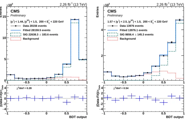
regions from simulated QCD multijet events. The distributions of BDT outputs for EB and EE photons in data are shown in Fig. 2 for photon ET between 200 and 220 GeV and jet|y| < 1.5.
The fit results with signal, background, and combined distributions and ratio of data over fit are shown. The fitted results match well with data distributions as shown in χ2over the degree of freedom, goodness-of-fit, in the residual ratio plot of data over fit results.
The corrected signal yield is unfolded using the iterative D’Agostini method [39], as imple-mented in the RooUnfold software package [40], to take into account migrations between dif-ferent bins due to the photon energy scale and resolution. The unfolding response matrix is obtained from thePYTHIA8 photon+jets sample. The unfolding corrections are small, of the or-der of 1%. The size of the corrections is also verified using an independent photon+jets sample generated with MADGRAPH.
BDT output -1 -0.5 0 0.5 1 arbitrary units 0 0.2 0.4 0.6 < 220 GeV T γ | < 1.44, 200 < E γ |y Data sideband MC signal region MC sideband (13 TeV) -1 2.26 fb
CMS
PreliminaryFigure 1: Distributions of the BDT for background photons in the 200–220 GeV bin for the EB region. The points show events from a sideband region of the photon isolation selection criteria, the solid histogram shows the events in the signal region in simulated QCD multijet events, and the dashed histogram shows the sideband region for simulated QCD multijet events. All three samples have their statistical uncertainties shown as error bars.
The inclusive isolated-photon differential production cross section is calculated as d2σ dyγdEγ T = U (N γ) ∆yγ∆Eγ T 1 eSF L, (1)
and the photon+jets as
d3σ dyγdEγ Tdyjet = U (N γ) ∆yγ∆Eγ T∆yjet 1 eSF L, (2)
whereU (Nγ)denotes the unfolded photon yields in bins of width ∆Eγ
T and∆y, and y is the
rapidity of either the photon or the jet. In these equations, e denotes the product of trigger, reconstruction, and selection efficiencies; SF the product of the selection and electron veto scale factors; and L is the integrated luminosity.
6
Systematic uncertainties
The uncertainty in the efficiency of the event selection is typically small except in the high-ET
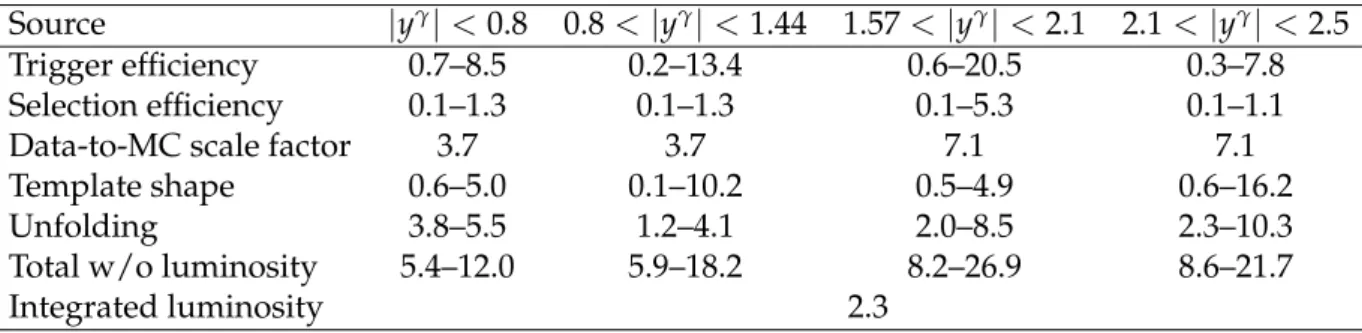
region, where statistical uncertainties in both data and simulated events dominate. A summary of the systematic uncertainties is given in Table 1.
The systematic uncertainties in the signal and background templates are incorporated into the fit as nuisance parameters. For the signal template uncertainty, the nuisance parameter is as-signed a Gaussian prior, while log-normal priors are asas-signed to the background template nui-sances. A description of the general methodology can be found in Ref. [41]. The bias correction,
BDT output 1 − −0.5 0 0.5 1 Entries 0 5 10 15 3 10 × < 220 GeV T γ | < 1.5, 200 < E jet | < 1.44, |y γ |y Data 28156 events Fitted 28159.5 events 183.6 events ± SIG 22638.3 Background (13 TeV) -1 2.26 fb CMS Preliminary BDT output 1 − −0.5 0 0.5 1 Data σ (Data-Fit)/ 4 − 2 − 0 2 4 χ2/dof = 0.28 BDT output 1 − −0.5 0 0.5 1 Entries 2 4 3 10 × < 220 GeV T γ | < 1.5, 200 < E jet | < 2.5, |y γ 1.57 < |y Data 13976 events Fitted 13976.1 events 145.3 events ± SIG 8656.4 Background (13 TeV) -1 2.26 fb CMS Preliminary BDT output 1 − −0.5 0 0.5 1 Data σ (Data-Fit)/ 4 − 2 − 0 2 4 χ2/dof = 0.54
Figure 2: Distributions of the BDT output for an EB (left) and an EE (right) bin with photon ET between 200–220 GeV and|yjet| <1.5. The points represent data, and the solid histograms,
approaching the data points, represent the fit results with the signal (dashed) and background (dotted) components displayed. The bottom panels show the ratio of the difference between the data and the fit to the statistical uncertainty in the data, along with the resulting reduced χ2over degrees of freedom (dof).
applied on the photon yields, due to the selection of the sideband range is also considered as a systematic uncertainty.
The impact on photon yields from the unfolding uncertainties, which include photon energy scale and resolution uncertainties, is roughly 5%. The uncertainties of the event selection effi-ciency due to the jet selection and jet rapidity migration are negligible.
The uncertainty in the measurement of the CMS integrated luminosity is 2.3% [19].
The total uncertainty in the yield per bin, excluding the highest photon ET bin in each y range,
is about 5–8% for EB and 9–17% for EE photons. The highest photon ET bins in all y region
have limited events in data and simulated samples for the evaluation of systematics.
7
Results and comparison with theory
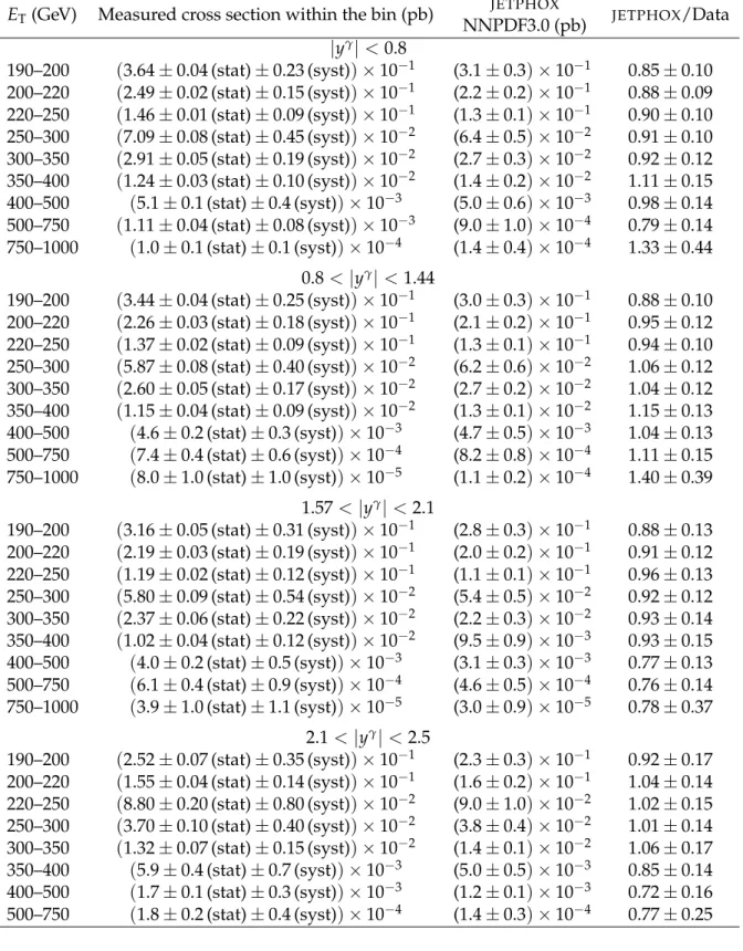
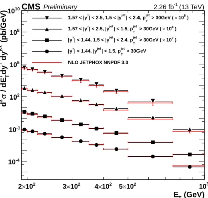
The measured inclusive isolated-photon and photon+jets cross sections are shown in Figs. 3 and 5, respectively, and in Tables 2 and 3.
The measured cross sections are compared with NLO perturbative QCD calculations from the
JETPHOX 1.3.1 generator [11, 42, 43], using the NNPDF3.0 NLO [13] PDFs and the Bourhis-Fontannaz-Guillet (BFG) set II parton fragmentation functions [44]. The renormalization, fac-torization, and fragmentation scales are all set to be equal to the photon ET. To estimate the
indepen-Table 1: Impact on cross sections, in percent, for each systematic uncertainty source in the four photon rapidity regions,|yγ| <0.8, 0.8< |yγ| <1.44, 1.57 < |yγ| <2.1, and 2.1< |yγ| <2.5.
The ranges, when quoted, indicate the variation over photon ETbetween 190–1000 GeV.
Source |yγ| <0.8 0.8< |yγ| <1.44 1.57< |yγ| <2.1 2.1< |yγ| <2.5
Trigger efficiency 0.7–8.5 0.2–13.4 0.6–20.5 0.3–7.8
Selection efficiency 0.1–1.3 0.1–1.3 0.1–5.3 0.1–1.1
Data-to-MC scale factor 3.7 3.7 7.1 7.1
Template shape 0.6–5.0 0.1–10.2 0.5–4.9 0.6–16.2
Unfolding 3.8–5.5 1.2–4.1 2.0–8.5 2.3–10.3
Total w/o luminosity 5.4–12.0 5.9–18.2 8.2–26.9 8.6–21.7
Integrated luminosity 2.3
dently from ET/2 to 2ET, while keeping their ratio between one-half and two. The impact of JETPHOX cross section predictions due to the uncertainties in the PDF and in the strong cou-pling αS=0.118 at the mass of Z boson is calculated using the 68% confidence level NNPDF3.0
NLO replica. The total theoretical uncertainties of the cross section predictions are evaluated as the quadratic sum of the scale, PDF, and αSuncertainties.
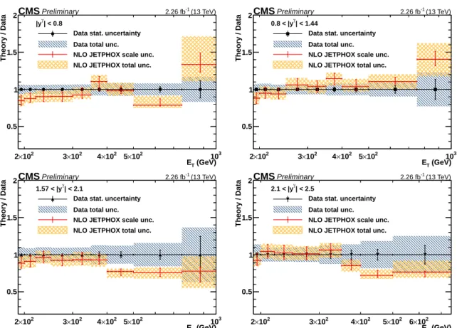
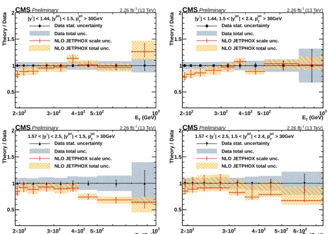
The ratio of the theoretical predictions to data, together with the experimental and theoretical uncertainties, are shown in Figs. 4 and 6 for the isolated-photon and photon+jets cross section measurements respectively. The uncertainties in the theoretical predictions and ratios to data are symmetrized in the tables; the largest value between the positive and negative uncertain-ties is listed. Measured cross sections are in agreement with theoretical expectations within statistical and systematic uncertainties.
The ratio of the theoretical predictions to data based on JETPHOX at NLO with different PDF
sets, including MMHT14 [14], CT14 [15], and HERAPDF2.0 [45] together with NNPDF3.0, are shown in Fig. 7. The differences between JETPHOX predictions using different PDF sets are
small, within the theoretical uncertainties estimated with NNPDF3.0.
8
Summary
The differential cross sections for inclusive isolated-photon and photon+jets production in proton-proton collisions at a center-of-mass energy of 13 TeV are measured with a data sample collected by the CMS experiment corresponding to an integrated luminosity of 2.26 fb−1. The measurements of inclusive isolated-photon production cross sections are presented as func-tions of photon transverse energy and rapidity. The photon+jets production cross secfunc-tions are presented as functions of photon transverse energy, and photon and jet rapidities.
The measurements are compared with theoretical predictions produced using theJETPHOX next-to-leading order calculations using different parton distribution functions. The theoretical pre-dictions agree with the experimental measurements within the statistical and systematic un-certainties. For low to middle range in photon ET, where the experimental uncertainties are
smaller or comparable to theoretical uncertainties, these measurements provide the potential to further constrain the proton PDFs. The agreement between data and theory, and the new next-to-next-to-leading-order (NNLO) calculations [46] motivate the use of additional mea-surements to better estimate the gluon and other PDFs.
Table 2: Measured and predicted differential cross section for isolated-photon production, along with the statistical and systematical uncertainties in the various ET and y bins.
Predic-tions useJETPHOXat NLO with the NNPDF3.0 PDF set. The ratio of theJETPHOXpredictions to data are listed in the last column, with the total uncertainty estimated assuming uncorrelated experimental and theoretical uncertainties.
ET(GeV) Measured cross section within the bin (pb) NNPDF3.0 (pb)JETPHOX JETPHOX/Data
|yγ| < 0.8 190–200 (3.64 ± 0.04 (stat) ± 0.23 (syst)) × 10−1 (3.1 ± 0.3) × 10−1 0.85 ± 0.10 200–220 (2.49 ± 0.02 (stat) ± 0.15 (syst)) × 10−1 (2.2 ± 0.2) × 10−1 0.88 ± 0.09 220–250 (1.46 ± 0.01 (stat) ± 0.09 (syst)) × 10−1 (1.3 ± 0.1) × 10−1 0.90 ± 0.10 250–300 (7.09 ± 0.08 (stat) ± 0.45 (syst)) × 10−2 (6.4 ± 0.5) × 10−2 0.91 ± 0.10 300–350 (2.91 ± 0.05 (stat) ± 0.19 (syst)) × 10−2 (2.7 ± 0.3) × 10−2 0.92 ± 0.12 350–400 (1.24 ± 0.03 (stat) ± 0.10 (syst)) × 10−2 (1.4 ± 0.2) × 10−2 1.11 ± 0.15 400–500 (5.1 ± 0.1 (stat) ± 0.4 (syst)) × 10−3 (5.0 ± 0.6) × 10−3 0.98 ± 0.14 500–750 (1.11 ± 0.04 (stat) ± 0.08 (syst)) × 10−3 (9.0 ± 1.0) × 10−4 0.79 ± 0.14 750–1000 (1.0 ± 0.1 (stat) ± 0.1 (syst)) × 10−4 (1.4 ± 0.4) × 10−4 1.33 ± 0.44 0.8 < |yγ| < 1.44 190–200 (3.44 ± 0.04 (stat) ± 0.25 (syst)) × 10−1 (3.0 ± 0.3) × 10−1 0.88 ± 0.10 200–220 (2.26 ± 0.03 (stat) ± 0.18 (syst)) × 10−1 (2.1 ± 0.2) × 10−1 0.95 ± 0.12 220–250 (1.37 ± 0.02 (stat) ± 0.09 (syst)) × 10−1 (1.3 ± 0.1) × 10−1 0.94 ± 0.10 250–300 (5.87 ± 0.08 (stat) ± 0.40 (syst)) × 10−2 (6.2 ± 0.6) × 10−2 1.06 ± 0.12 300–350 (2.60 ± 0.05 (stat) ± 0.17 (syst)) × 10−2 (2.7 ± 0.2) × 10−2 1.04 ± 0.12 350–400 (1.15 ± 0.04 (stat) ± 0.09 (syst)) × 10−2 (1.3 ± 0.1) × 10−2 1.15 ± 0.13 400–500 (4.6 ± 0.2 (stat) ± 0.3 (syst)) × 10−3 (4.7 ± 0.5) × 10−3 1.04 ± 0.13 500–750 (7.4 ± 0.4 (stat) ± 0.6 (syst)) × 10−4 (8.2 ± 0.8) × 10−4 1.11 ± 0.15 750–1000 (8.0 ± 1.0 (stat) ± 1.0 (syst)) × 10−5 (1.1 ± 0.2) × 10−4 1.40 ± 0.39 1.57 < |yγ| < 2.1 190–200 (3.16 ± 0.05 (stat) ± 0.31 (syst)) × 10−1 (2.8 ± 0.3) × 10−1 0.88 ± 0.13 200–220 (2.19 ± 0.03 (stat) ± 0.19 (syst)) × 10−1 (2.0 ± 0.2) × 10−1 0.91 ± 0.12 220–250 (1.19 ± 0.02 (stat) ± 0.12 (syst)) × 10−1 (1.1 ± 0.1) × 10−1 0.96 ± 0.13 250–300 (5.80 ± 0.09 (stat) ± 0.54 (syst)) × 10−2 (5.4 ± 0.5) × 10−2 0.92 ± 0.12 300–350 (2.37 ± 0.06 (stat) ± 0.22 (syst)) × 10−2 (2.2 ± 0.3) × 10−2 0.93 ± 0.14 350–400 (1.02 ± 0.04 (stat) ± 0.12 (syst)) × 10−2 (9.5 ± 0.9) × 10−3 0.93 ± 0.15 400–500 (4.0 ± 0.2 (stat) ± 0.5 (syst)) × 10−3 (3.1 ± 0.3) × 10−3 0.77 ± 0.13 500–750 (6.1 ± 0.4 (stat) ± 0.9 (syst)) × 10−4 (4.6 ± 0.5) × 10−4 0.76 ± 0.14 750–1000 (3.9 ± 1.0 (stat) ± 1.1 (syst)) × 10−5 (3.0 ± 0.9) × 10−5 0.78 ± 0.37 2.1 < |yγ| < 2.5 190–200 (2.52 ± 0.07 (stat) ± 0.35 (syst)) × 10−1 (2.3 ± 0.3) × 10−1 0.92 ± 0.17 200–220 (1.55 ± 0.04 (stat) ± 0.14 (syst)) × 10−1 (1.6 ± 0.2) × 10−1 1.04 ± 0.14 220–250 (8.80 ± 0.20 (stat) ± 0.80 (syst)) × 10−2 (9.0 ± 1.0) × 10−2 1.02 ± 0.15 250–300 (3.70 ± 0.10 (stat) ± 0.40 (syst)) × 10−2 (3.8 ± 0.4) × 10−2 1.01 ± 0.14 300–350 (1.32 ± 0.07 (stat) ± 0.15 (syst)) × 10−2 (1.4 ± 0.1) × 10−2 1.06 ± 0.17 350–400 (5.9 ± 0.4 (stat) ± 0.7 (syst)) × 10−3 (5.0 ± 0.5) × 10−3 0.85 ± 0.14 400–500 (1.7 ± 0.1 (stat) ± 0.3 (syst)) × 10−3 (1.2 ± 0.1) × 10−3 0.72 ± 0.16 500–750 (1.8 ± 0.2 (stat) ± 0.4 (syst)) × 10−4 (1.4 ± 0.3) × 10−4 0.77 ± 0.25
Table 3: Measured and predicted differential cross section for photon+jets production, along with statistical and systematical uncertainties in the various ET and y bins. Predictions are
based onJETPHOXat NLO with the NNPDF3.0 PDF set. The ratio of theJETPHOXpredictions to the data are listed in the last column, with the total uncertainty estimated assuming uncor-related experimental and theoretical uncertainties.
ET(GeV) Measured cross section within the bin (pb) NNPDF3.0 (pb)JETPHOX JETPHOX/Data
|yγ| < 1.44, |yjet| < 1.5, and pjet
T > 30 GeV 190–200 (9.20 ± 0.10 (stat) ± 0.60 (syst)) × 10−2 (7.7 ± 0.7) × 10−2 0.83 ± 0.10 200–220 (6.26 ± 0.06 (stat) ± 0.41 (syst)) × 10−2 (5.6 ± 0.5) × 10−2 0.89 ± 0.10 220–250 (3.72 ± 0.04 (stat) ± 0.23 (syst)) × 10−2 (3.3 ± 0.3) × 10−2 0.89 ± 0.10 250–300 (1.72 ± 0.02 (stat) ± 0.11 (syst)) × 10−2 (1.6 ± 0.2) × 10−2 0.95 ± 0.12 300–350 (7.50 ± 0.10 (stat) ± 0.50 (syst)) × 10−3 (7.3 ± 0.7) × 10−3 0.97 ± 0.11 350–400 (3.34 ± 0.08 (stat) ± 0.25 (syst)) × 10−3 (3.8 ± 0.4) × 10−3 1.14 ± 0.15 400–500 (1.37 ± 0.03 (stat) ± 0.10 (syst)) × 10−3 (1.4 ± 0.1) × 10−3 1.02 ± 0.12 500–750 (2.82 ± 0.09 (stat) ± 0.22 (syst)) × 10−4 (2.7 ± 0.2) × 10−4 0.97 ± 0.12 750–1000 (3.0 ± 0.3 (stat) ± 0.3 (syst)) × 10−5 (3.8 ± 0.6) × 10−5 1.26 ± 0.26
|yγ| < 1.44, 1.5 < |yjet| < 2.4, and pjet
T > 30 GeV 190–200 (4.08 ± 0.09 (stat) ± 0.27 (syst)) × 10−2 (3.2 ± 0.4) × 10−2 0.78 ± 0.11 200–220 (2.73 ± 0.05 (stat) ± 0.18 (syst)) × 10−2 (2.3 ± 0.2) × 10−2 0.84 ± 0.10 220–250 (1.54 ± 0.03 (stat) ± 0.10 (syst)) × 10−2 (1.3 ± 0.1) × 10−2 0.86 ± 0.10 250–300 (6.90 ± 0.10 (stat) ± 0.50 (syst)) × 10−3 (6.3 ± 0.6) × 10−3 0.91 ± 0.10 300–350 (2.73 ± 0.09 (stat) ± 0.18 (syst)) × 10−3 (2.7 ± 0.3) × 10−3 0.97 ± 0.12 350–400 (1.12 ± 0.05 (stat) ± 0.08 (syst)) × 10−3 (1.2 ± 0.1) × 10−3 1.07 ± 0.13 400–500 (4.4 ± 0.2 (stat) ± 0.3 (syst)) × 10−4 (3.9 ± 0.3) × 10−4 0.89 ± 0.10 500–750 (5.8 ± 0.5 (stat) ± 0.5 (syst)) × 10−5 (6.0 ± 0.6) × 10−5 1.03 ± 0.15 750–1000 (4.3 ± 1.3 (stat) ± 0.4 (syst)) × 10−6 (4.4 ± 0.7) × 10−6 1.02 ± 0.36 1.57 < |yγ| < 2.5, |yjet| < 1.5, and pjet
T > 30 GeV 190–200 (6.00 ± 0.10 (stat) ± 0.60 (syst)) × 10−2 (5.1 ± 0.6) × 10−2 0.85 ± 0.12 200–220 (3.92 ± 0.08 (stat) ± 0.39 (syst)) × 10−2 (3.6 ± 0.4) × 10−2 0.92 ± 0.14 220–250 (2.42 ± 0.04 (stat) ± 0.23 (syst)) × 10−2 (2.1 ± 0.2) × 10−2 0.88 ± 0.13 250–300 (1.08 ± 0.02 (stat) ± 0.12 (syst)) × 10−2 (1.0 ± 0.1) × 10−2 0.93 ± 0.14 300–350 (4.70 ± 0.10 (stat) ± 0.50 (syst)) × 10−3 (4.2 ± 0.4) × 10−3 0.90 ± 0.13 350–400 (2.03 ± 0.09 (stat) ± 0.25 (syst)) × 10−3 (1.8 ± 0.2) × 10−3 0.91 ± 0.15 400–500 (8.1 ± 0.3 (stat) ± 0.9 (syst)) × 10−4 (6.0 ± 0.5) × 10−4 0.74 ± 0.11 500–750 (1.24 ± 0.08 (stat) ± 0.17 (syst)) × 10−4 (8.5 ± 0.9) × 10−5 0.69 ± 0.12 750–1000 (1.0 ± 0.2 (stat) ± 0.3 (syst)) × 10−5 (6.0 ± 2.0) × 10−6 0.64 ± 0.32
1.57 < |yγ| < 2.5, 1.5 < |yjet| < 2.4, and pjet
T > 30 GeV 190–200 (5.00 ± 0.10 (stat) ± 0.50 (syst)) × 10−2 (4.0 ± 1.0) × 10−2 0.85 ± 0.23 200–220 (3.39 ± 0.08 (stat) ± 0.34 (syst)) × 10−2 (3.0 ± 0.8) × 10−2 0.89 ± 0.24 220–250 (1.87 ± 0.05 (stat) ± 0.17 (syst)) × 10−2 (1.7 ± 0.5) × 10−2 0.91 ± 0.26 250–300 (8.1 ± 0.2 (stat) ± 0.9 (syst)) × 10−3 (7.0 ± 2.0) × 10−3 0.92 ± 0.27 300–350 (3.4 ± 0.1 (stat) ± 0.3 (syst)) × 10−3 (2.8 ± 0.8) × 10−3 0.83 ± 0.26 350–400 (1.38 ± 0.02 (stat) ± 0.17 (syst)) × 10−3 (1.0 ± 0.3) × 10−3 0.74 ± 0.25 400–500 (3.4 ± 0.3 (stat) ± 0.4 (syst)) × 10−4 (2.7 ± 0.8) × 10−4 0.79 ± 0.27 500–750 (4.1 ± 0.7 (stat) ± 0.5 (syst)) × 10−5 (3.0 ± 1.0) × 10−5 0.67 ± 0.30
(GeV) T E 2 10 × 2 3×10² 4×10² 5×10² 3 10 (pb/GeV) γ dy T γ / dE σ 2 d -3 10 1 3 10 6 10 9 10 ) 6 10 × | < 2.5 ( γ 2.1 < |y ) 4 10 × | < 2.1 ( γ 1.57 < |y ) 2 10 × | < 1.44 ( γ 0.8 < |y | < 0.8 γ |y NLO JETPHOX NNPDF 3.0 (13 TeV) -1 2.26 fb CMSPreliminary
Figure 3: Differential cross sections for isolated-photon production in photon rapidity bins, |yγ| < 0.8, 0.8 < |yγ| < 1.44, 1.57 < |yγ| < 2.1, and 2.1 < |yγ| < 2.5. The points show the
measured values and their total uncertainties; the lines show the NLO JETPHOX predictions
(GeV) T E 2 10 × 2 3×10² 4×10² 5×10² 103 Theory / Data 0.5 1 1.5 2 | < 0.8 γ |y
Data stat. uncertainty Data total unc. NLO JETPHOX scale unc. NLO JETPHOX total unc.
(13 TeV) -1 2.26 fb CMSPreliminary (GeV) T E 2 10 × 2 3×10² 4×10² 5×10² 103 Theory / Data 0.5 1 1.5 2 | < 1.44 γ 0.8 < |y
Data stat. uncertainty Data total unc. NLO JETPHOX scale unc. NLO JETPHOX total unc.
(13 TeV) -1 2.26 fb CMSPreliminary (GeV) T E 2 10 × 2 3×10² 4×10² 5×10² 3 10 Theory / Data 0.5 1 1.5 2 | < 2.1 γ 1.57 < |y
Data stat. uncertainty Data total unc. NLO JETPHOX scale unc. NLO JETPHOX total unc.
(13 TeV) -1 2.26 fb CMSPreliminary (GeV) T E 2 10 × 2 3×10² 4×10² 5×10² 6×10² Theory / Data 0.5 1 1.5 2 | < 2.5 γ 2.1 < |y
Data stat. uncertainty Data total unc. NLO JETPHOX scale unc. NLO JETPHOX total unc.
(13 TeV)
-1
2.26 fb
CMSPreliminary
Figure 4: The ratios of theoretical NLO predictions to data for the differential cross sections for isolated-photon production in four photon rapidity bins, |yγ| < 0.8, 0.8 < |yγ| < 1.44,
1.57 < |yγ| < 2.1, and 2.1 < |yγ| < 2.5, are shown. The error bars on data points represent
the statistical uncertainty, while the hatched area shows the total experimental uncertainty. The errors on the ratio represent scale uncertainties, and the shaded regions represent the total theoretical uncertainties.
(GeV) T E 2 10 × 2 3×10² 4×10² 5×10² 3 10 (pb/GeV) jet dy γ dy T γ / dE σ 3 d -4 10 -1 10 2 10 5 10 8 10 10 10 ) 6 10 × > 30GeV ( jet T | < 2.4, p jet | < 2.5, 1.5 < |y γ 1.57 < |y ) 4 10 × > 30GeV ( jet T | < 1.5, p jet | < 2.5, |y γ 1.57 < |y ) 2 10 × > 30GeV ( jet T | < 2.4, p jet | < 1.44, 1.5 < |y γ |y > 30GeV jet T | < 1.5, p jet | < 1.44, |y γ |y NLO JETPHOX NNPDF 3.0 (13 TeV) -1 2.26 fb CMSPreliminary
Figure 5: Differential cross sections for photon+jets production in two photon rapidity bins, |yγ| < 1.44 and 1.57 < |yγ| <2.5, and two jet rapidity bins,|yjet| < 1.5 and 1.5< |yjet| < 2.4.
The points show the measured values with their total uncertainties, and the lines show the NLOJETPHOXpredictions with the NNPDF3.0 PDF set.
(GeV) T E 2 10 × 2 3×10² 4×10² 5×10² 103 Theory / Data 0.5 1 1.5 2 > 30GeV jet T | < 1.5, p jet | < 1.44, |y γ |y
Data stat. uncertainty Data total unc. NLO JETPHOX scale unc. NLO JETPHOX total unc.
(13 TeV) -1 2.26 fb CMSPreliminary (GeV) T E 2 10 × 2 3×10² 4×10² 5×10² 103 Theory / Data 0.5 1 1.5 2 > 30GeV jet T | < 2.4, p jet | < 1.44, 1.5 < |y γ |y
Data stat. uncertainty Data total unc. NLO JETPHOX scale unc. NLO JETPHOX total unc.
(13 TeV) -1 2.26 fb CMSPreliminary (GeV) T E 2 10 × 2 3×10² 4×10² 5×10² 3 10 Theory / Data 0.5 1 1.5 2 > 30GeV jet T | < 1.5, p jet | < 2.5, |y γ 1.57 < |y
Data stat. uncertainty Data total unc. NLO JETPHOX scale unc. NLO JETPHOX total unc.
(13 TeV) -1 2.26 fb CMSPreliminary (GeV) T E 2 10 × 2 3×10² 4×10² 5×10² 6×10² Theory / Data 0.5 1 1.5 2 > 30GeV jet T | < 2.4, p jet | < 2.5, 1.5 < |y γ 1.57 < |y
Data stat. uncertainty Data total unc. NLO JETPHOX scale unc. NLO JETPHOX total unc.
(13 TeV)
-1
2.26 fb
CMSPreliminary
Figure 6: The ratios of theoretical NLO prediction to data for the differential cross sections for photon+jets production in two photon rapidity (|yγ| <1.44 and 1.57< |yγ| <2.5) and two jet
rapidity (|yjet| <1.5 and 1.5< |yjet| <2.4) bins , are shown. The error bars on the data points represent their statistical uncertainty, while the hatched area shows the total experimental un-certainty. The error bars on the ratios show the scale uncertainties, and the shaded area shows the total theoretical uncertainties.
(GeV) T E 2 10 × 2 3×10² 4×10² 5×10² 103 Theory / Data 0.5 1 1.5 2 (13 TeV) -1 2.26 fb CMSPreliminary | < 0.8 γ |y
Data experimental unc. NLO JETPHOX NNPDF3.0 NLO JETPHOX CT14 NLO JETPHOX MMHT14 NLO JETPHOX HERAPDF2.0 NNPDF3.0 total theoretical unc.
(GeV) T E 2 10 × 2 3×10² 4×10² 5×10² 103 Theory / Data 0.5 1 1.5 2 (13 TeV) -1 2.26 fb CMSPreliminary | < 1.44 γ 0.8 < |y
Data experimental unc. NLO JETPHOX NNPDF3.0 NLO JETPHOX CT14 NLO JETPHOX MMHT14 NLO JETPHOX HERAPDF2.0 NNPDF3.0 total theoretical unc.
(GeV) T E 2 10 × 2 3×10² 4×10² 5×10² 3 10 Theory / Data 0.5 1 1.5 2 (13 TeV) -1 2.26 fb CMSPreliminary | < 2.1 γ 1.57 < |y
Data experimental unc. NLO JETPHOX NNPDF3.0 NLO JETPHOX CT14 NLO JETPHOX MMHT14 NLO JETPHOX HERAPDF2.0 NNPDF3.0 total theoretical unc.
(GeV) T E 2 10 × 2 3×10² 4×10² 5×10² 6×10² Theory / Data 0.5 1 1.5 2 (13 TeV) -1 2.26 fb CMSPreliminary | < 2.5 γ 2.1 < |y
Data experimental unc. NLO JETPHOX NNPDF3.0 NLO JETPHOX CT14 NLO JETPHOX MMHT14 NLO JETPHOX HERAPDF2.0 NNPDF3.0 total theoretical unc.
(GeV) T E 2 10 × 2 3×10² 4×10² 5×10² 103 Theory / Data 0.5 1 1.5 2 (13 TeV) -1 2.26 fb CMSPreliminary > 30GeV jet T | < 1.5, p jet | < 1.44, |y γ |y
Data experimental unc. NLO JETPHOX NNPDF3.0 NLO JETPHOX CT14 NO JETPHOX MMHT14 NLO JETPHOX HERAPDF2.0 NNPDF3.0 total theoretical unc.
(GeV) T E 2 10 × 2 3×10² 4×10² 5×10² 103 Theory / Data 0.5 1 1.5 2 (13 TeV) -1 2.26 fb CMSPreliminary > 30GeV jet T | < 2.4, p jet | < 1.44, 1.5 < |y γ |y
Data experimental unc. NLO JETPHOX NNPDF3.0 NLO JETPHOX CT14 NO JETPHOX MMHT14 NLO JETPHOX HERAPDF2.0 NNPDF3.0 total theoretical unc.
(GeV) T E 2 10 × 2 3×10² 4×10² 5×10² 3 10 Theory / Data 0.5 1 1.5 2 (13 TeV) -1 2.26 fb CMSPreliminary > 30GeV jet T | < 1.5, p jet | < 2.5, |y γ 1.57 < |y
Data experimental unc. NLO JETPHOX NNPDF3.0 NLO JETPHOX CT14 NO JETPHOX MMHT14 NLO JETPHOX HERAPDF2.0 NNPDF3.0 total theoretical unc.
(GeV) T E 2 10 × 2 3×10² 4×10² 5×10² 6×10² Theory / Data 0.5 1 1.5 2 (13 TeV) -1 2.26 fb CMSPreliminary > 30GeV jet T | < 2.4, p jet | < 2.5, 1.5 < |y γ 1.57 < |y
Data experimental unc. NLO JETPHOX NNPDF3.0 NLO JETPHOX CT14 NO JETPHOX MMHT14 NLO JETPHOX HERAPDF2.0 NNPDF3.0 total theoretical unc.
Figure 7: Ratios of JETPHOX NLO predictions to data for various PDF sets as a function of
photon ET for inclusive isolated-photons (top four panels) and photon+jets (four bottom
pan-els). Data are shown as points, the error bars represent statistical uncertainties, while the hatched area represents the total experimental uncertainties. The theoretical uncertainty in the NNPDF3.0 prediction is shown as a shaded area.
Acknowledgments
We congratulate our colleagues in the CERN accelerator departments for the excellent perfor-mance of the LHC and thank the technical and administrative staffs at CERN and at other CMS institutes for their contributions to the success of the CMS effort. In addition, we gratefully acknowledge the computing centres and personnel of the Worldwide LHC Computing Grid for delivering so effectively the computing infrastructure essential to our analyses. Finally, we acknowledge the enduring support for the construction and operation of the LHC and the CMS detector provided by the following funding agencies: BMWFW and FWF (Austria); FNRS and FWO (Belgium); CNPq, CAPES, FAPERJ, and FAPESP (Brazil); MES (Bulgaria); CERN; CAS, MoST, and NSFC (China); COLCIENCIAS (Colombia); MSES and CSF (Croatia); RPF (Cyprus); SENESCYT (Ecuador); MoER, ERC IUT, and ERDF (Estonia); Academy of Finland, MEC, and HIP (Finland); CEA and CNRS/IN2P3 (France); BMBF, DFG, and HGF (Germany); GSRT (Greece); OTKA and NIH (Hungary); DAE and DST (India); IPM (Iran); SFI (Ireland); INFN (Italy); MSIP and NRF (Republic of Korea); LAS (Lithuania); MOE and UM (Malaysia); BUAP, CINVESTAV, CONACYT, LNS, SEP, and UASLP-FAI (Mexico); MBIE (New Zealand); PAEC (Pakistan); MSHE and NSC (Poland); FCT (Portugal); JINR (Dubna); MON, RosAtom, RAS, and RFBR (Russia); MESTD (Serbia); SEIDI and CPAN (Spain); Swiss Funding Agencies (Switzerland); MST (Taipei); ThEPCenter, IPST, STAR, and NSTDA (Thailand); TUBITAK and TAEK (Turkey); NASU and SFFR (Ukraine); STFC (United Kingdom); DOE and NSF (USA). Individuals have received support from the Marie-Curie programme and the European Re-search Council and Horizon 2020 Grant, contract No. 675440 (European Union); the Leventis Foundation; the A. P. Sloan Foundation; the Alexander von Humboldt Foundation; the Belgian Federal Science Policy Office; the Fonds pour la Formation `a la Recherche dans l’Industrie et dans l’Agriculture (FRIA-Belgium); the Agentschap voor Innovatie door Wetenschap en Tech-nologie (IWT-Belgium); the F.R.S.-FNRS and FWO (Belgium) under the “Excellence of Science - EOS” - be.h project n. 30820817; the Ministry of Education, Youth and Sports (MEYS) of the Czech Republic; the Lend ¨ulet (“Momentum”) Programme and the J´anos Bolyai Research Schol-arship of the Hungarian Academy of Sciences, the New National Excellence Program ´UNKP, the NKFIA research grants 123842, 123959, 124845, 124850 and 125105 (Hungary); the Council of Science and Industrial Research, India; the HOMING PLUS programme of the Foundation for Polish Science, cofinanced from European Union, Regional Development Fund, the Mo-bility Plus programme of the Ministry of Science and Higher Education, the National Science Center (Poland), contracts Harmonia 2014/14/M/ST2/00428, Opus 2014/13/B/ST2/02543, 2014/15/B/ST2/03998, and 2015/19/B/ST2/02861, Sonata-bis 2012/07/E/ST2/01406; the National Priorities Research Program by Qatar National Research Fund; the Programa Estatal de Fomento de la Investigaci ´on Cient´ıfica y T´ecnica de Excelencia Mar´ıa de Maeztu, grant MDM-2015-0509 and the Programa Severo Ochoa del Principado de Asturias; the Thalis and Aristeia programmes cofinanced by EU-ESF and the Greek NSRF; the Rachadapisek Sompot Fund for Postdoctoral Fellowship, Chulalongkorn University and the Chulalongkorn Aca-demic into Its 2nd Century Project Advancement Project (Thailand); the Welch Foundation, contract C-1845; and the Weston Havens Foundation (USA).
References
[1] CMS Collaboration, “Measurement of the isolated prompt photon production cross section in pp collisions at√s =7 TeV”, Phys. Rev. Lett. 106 (2011) 082001,
[2] CMS Collaboration, “Measurement of the differential cross section for isolated prompt photon production in pp collisions at 7 TeV”, Phys. Rev. D 84 (2011) 052011,
doi:10.1103/PhysRevD.84.052011, arXiv:1108.2044.
[3] CMS Collaboration, “Measurement of isolated photon production in pp and PbPb collisions at√sNN=2.76 TeV”, Phys. Lett. B 710 (2012) 256,
doi:10.1016/j.physletb.2012.02.077, arXiv:1201.3093.
[4] ATLAS Collaboration, “Measurement of the inclusive isolated prompt photons cross section in pp collisions at√s =7 TeV with the ATLAS detector using 4.6 fb−1”, Phys. Rev. D 89 (2014) 052004, doi:10.1103/PhysRevD.89.052004, arXiv:1311.1440. [5] ATLAS Collaboration, “Measurement of the inclusive isolated prompt photon cross
section in pp collisions at√s =8 TeV with the ATLAS detector”, JHEP 08 (2016) 005, doi:10.1007/JHEP08(2016)005, arXiv:1605.03495.
[6] CMS Collaboration, “Measurement of the triple-differential cross section for photon+jets production in proton-proton collisions at√s=7 TeV”, JHEP 06 (2014) 009,
doi:10.1007/JHEP06(2014)009, arXiv:1311.6141.
[7] ATLAS Collaboration, “Measurement of the production cross section of an isolated photon associated with jets in proton-proton collisions at√s=7 TeV with the ATLAS detector”, Phys. Rev. D 85 (2012) 092014, doi:10.1103/PhysRevD.85.092014,
arXiv:1203.3161.
[8] ATLAS Collaboration, “High-E√ Tisolated-photon plus jets production in pp collisions at
s =8 TeV with the ATLAS detector”, Nucl. Phys. B 918 (2017) 257, doi:10.1016/j.nuclphysb.2017.03.006, arXiv:1611.06586.
[9] ATLAS Collaboration, “Measurement of the cross section for inclusive isolated-photon production in pp collisions at√s =13 TeV using the ATLAS detector”, Phys. Lett. B 770 (2017) 473, doi:10.1016/j.physletb.2017.04.072, arXiv:1701.06882.
[10] ATLAS Collaboration, “Measurement of the cross section for isolated-photon plus jet production in pp collisions at√s =13 TeV using the ATLAS detector”, Phys. Lett. B 780 (2017) 578, doi:10.1016/j.physletb.2018.03.035, arXiv:1801.00112.
[11] P. Aurenche et al., “A new critical study of photon production in hadronic collisions”, Phys. Rev. D 73 (2006) 094007, doi:10.1103/PhysRevD.73.094007,
arXiv:hep-ph/0602133.
[12] R. Ichou and D. d’Enterria, “Sensitivity of isolated photon production at TeV hadron colliders to the gluon distribution in the proton”, Phys. Rev. D 82 (2010) 014015,
doi:10.1103/PhysRevD.82.014015, arXiv:1005.4529.
[13] NNPDF Collaboration, “Parton distributions for the LHC Run II”, JHEP 04 (2015) 040, doi:10.1007/JHEP04(2015)040, arXiv:1410.8849.
[14] L. A. Harland-Lang, A. D. Martin, P. Motylinski, and R. S. Thorne, “Parton distributions in the LHC era: MMHT 2014 PDFs”, Eur. Phys. J. C 75 (2015) 204,
doi:10.1140/epjc/s10052-015-3397-6, arXiv:1412.3989.
[15] S. Dulat et al., “New parton distribution functions from a global analysis of quantum chromodynamics”, Phys. Rev. D 93 (2016) 033006,
[16] W. Vogelsang and A. Vogt, “Constraints on the proton’s gluon distribution from prompt photon production”, Nucl. Phys. B 453 (1995) 334,
doi:10.1016/0550-3213(95)00424-Q, arXiv:hep-ph/9505404.
[17] D. d’Enterria and J. Rojo, “Quantitative constraints on the gluon distribution function in the proton from collider isolated-photon data”, Nucl. Phys. B 860 (2012) 311,
doi:10.1016/j.nuclphysb.2012.03.003, arXiv:1202.1762.
[18] L. Carminati et al., “Sensitivity of the LHC isolated-gamma+jet data to the parton distribution functions of the proton”, EPL 101 (2013) 61002,
doi:10.1209/0295-5075/101/61002, arXiv:1212.5511.
[19] CMS Collaboration, “CMS luminosity measurement for the 2015 data-taking period”, CMS Physics Analysis Summary CMS-PAS-LUM-15-001, 2016.
[20] H. Voss, A. H ¨ocker, J. Stelzer, and F. Tegenfeldt, “TMVA, the toolkit for multivariate data analysis with ROOT”, in XIth International Workshop on Advanced Computing and Analysis Techniques in Physics Research (ACAT), p. 40. 2007. arXiv:physics/0703039.
doi:10.22323/1.050.0040.
[21] CMS Collaboration, “The CMS Experiment at the CERN LHC”, JINST 3 (2008) S08004,
doi:10.1088/1748-0221/3/08/S08004.
[22] CMS Collaboration, “Description and performance of track and primary-vertex reconstruction with the CMS tracker”, JINST 9 (2014) P10009,
doi:10.1088/1748-0221/9/10/P10009, arXiv:1405.6569.
[23] CMS Collaboration, “Particle-flow reconstruction and global event description with the CMS detector”, JINST 12 (2017) P10003, doi:10.1088/1748-0221/12/10/P10003,
arXiv:1706.04965.
[24] CMS Collaboration, “Energy calibration and resolution of the CMS electromagnetic calorimeter in pp collisions at√s=7 TeV”, JINST 8 (2013) P09009,
doi:10.1088/1748-0221/8/09/P09009, arXiv:1306.2016.
[25] CMS Collaboration, “Performance of photon reconstruction and identification with the CMS detector in proton-proton collisions at√s=8 TeV”, JINST 10 (2015) P08010,
doi:10.1088/1748-0221/10/08/P08010, arXiv:1502.02702.
[26] M. Cacciari, G. P. Salam, and G. Soyez, “The anti-kTjet clustering algorithm”, JHEP 04
(2008) 063, doi:10.1088/1126-6708/2008/04/063, arXiv:0802.1189.
[27] M. Cacciari, G. P. Salam, and G. Soyez, “FastJet user manual”, Eur. Phys. J. C 72 (2012) 1896, doi:10.1140/epjc/s10052-012-1896-2, arXiv:1111.6097.
[28] CMS Collaboration, “Determination of jet energy calibration and transverse momentum resolution in CMS”, JINST 6 (2011) P11002,
doi:10.1088/1748-0221/6/11/P11002, arXiv:1107.4277.
[29] T. Sj ¨ostrand et al., “An Introduction to PYTHIA 8.2”, Comput. Phys. Commun. 191 (2015) 159, doi:10.1016/j.cpc.2015.01.024, arXiv:1410.3012.
[30] J. Alwall et al., “The automated computation of tree-level and next-to-leading order differential cross sections, and their matching to parton shower simulations”, JHEP 07 (2014) 079, doi:10.1007/JHEP07(2014)079, arXiv:1405.0301.
[31] J. Alwall et al., “Comparative study of various algorithms for the merging of parton showers and matrix elements in hadronic collisions”, Eur. Phys. J. C 53 (2008) 473, doi:10.1140/epjc/s10052-007-0490-5, arXiv:0706.2569.
[32] R. Frederix and S. Frixione, “Merging meets matching in MC@NLO”, JHEP 12 (2012) 061, doi:10.1007/JHEP12(2012)061, arXiv:1209.6215.
[33] CMS Collaboration, “Event generator tunes obtained from underlying event and multiparton scattering measurements”, Eur. Phys. J. C 76 (2016) 155,
doi:10.1140/epjc/s10052-016-3988-x, arXiv:1512.00815.
[34] NNPDF Collaboration, “Parton distributions with LHC data”, Nucl. Phys. B 867 (2013) 244, doi:10.1016/j.nuclphysb.2012.10.003, arXiv:1207.1303.
[35] GEANT4 Collaboration, “GEANT4—a simulation toolkit”, Nucl. Instrum. Meth. A 506 (2003) 250, doi:10.1016/S0168-9002(03)01368-8.
[36] CMS Collaboration, “The CMS trigger system”, JINST 12 (2017) P01020,
doi:10.1088/1748-0221/12/01/P01020, arXiv:1609.02366.
[37] CMS Collaboration, “Performance of missing energy reconstruction in 13 TeV pp collision data using the CMS detector”, CMS Physics Analysis Summary CMS-PAS-JME-16-004, 2016.
[38] CMS Collaboration, “Jet algorithms performance in 13 TeV data”, CMS Physics Analysis Summary CMS-PAS-JME-16-003, 2017.
[39] G. D’Agostini, “A multidimensional unfolding method based on Bayes’ theorem”, Nucl. Instrum. Meth. A 362 (1995) 487, doi:10.1016/0168-9002(95)00274-X.
[40] T. Adye, “Unfolding algorithms and tests using RooUnfold”, Proceedings, PHYSTAT 2011 Workshop on Statistical Issues Related to Discovery Claims in Search Experiments and Unfolding (2011) 313, doi:10.5170/CERN-2011-006.313, arXiv:1105.1160.
[41] ATLAS and CMS Collaborations, LHC Higgs Combination Group, “Procedure for the LHC Higgs boson search combination in summer 2011”, CMS/ATLAS joint note ATL-PHYS-PUB-2011-11, CMS NOTE 2011/005, 2011.
[42] S. Catani, M. Fontannaz, J. P. Guillet, and E. Pilon, “Cross section of isolated prompt photons in hadron-hadron collisions”, JHEP 05 (2002) 028,
doi:10.1088/1126-6708/2002/05/028, arXiv:hep-ph/0204023.
[43] Z. Belghobsi et al., “Photon-jet correlations and constraints on fragmentation functions”, Phys. Rev. D 79 (2009) 114024, doi:10.1103/PhysRevD.79.114024,
arXiv:0903.4834.
[44] L. Bourhis, M. Fontannaz, and J. P. Guillet, “Quark and gluon fragmentation functions into photons”, Eur. Phys. J. C 2 (1998) 529, doi:10.1007/s100520050158,
arXiv:hep-ph/9704447.
[45] H1 and ZEUS Collaborations, “Combination of measurements of inclusive deep inelastic e±p scattering cross sections and QCD analysis of HERA data”, Eur. Phys. J. C 75 (2015) 580, doi:10.1140/epjc/s10052-015-3710-4, arXiv:1506.06042.
[46] J. M. Campbell, R. K. Ellis, and C. Williams, “Direct photon production at next-to-next-to-leading order”, Phys. Rev. Lett. 118 (2017) 222001,
A
The CMS Collaboration
Yerevan Physics Institute, Yerevan, Armenia
A.M. Sirunyan, A. Tumasyan
Institut f ¨ur Hochenergiephysik, Wien, Austria
W. Adam, F. Ambrogi, E. Asilar, T. Bergauer, J. Brandstetter, E. Brondolin, M. Dragicevic, J. Er ¨o, A. Escalante Del Valle, M. Flechl, R. Fr ¨uhwirth1, V.M. Ghete, J. Hrubec, M. Jeitler1, N. Krammer, I. Kr¨atschmer, D. Liko, T. Madlener, I. Mikulec, N. Rad, H. Rohringer, J. Schieck1, R. Sch ¨ofbeck,
M. Spanring, D. Spitzbart, A. Taurok, W. Waltenberger, J. Wittmann, C.-E. Wulz1, M. Zarucki
Institute for Nuclear Problems, Minsk, Belarus
V. Chekhovsky, V. Mossolov, J. Suarez Gonzalez
Universiteit Antwerpen, Antwerpen, Belgium
E.A. De Wolf, D. Di Croce, X. Janssen, J. Lauwers, M. Pieters, M. Van De Klundert, H. Van Haevermaet, P. Van Mechelen, N. Van Remortel
Vrije Universiteit Brussel, Brussel, Belgium
S. Abu Zeid, F. Blekman, J. D’Hondt, I. De Bruyn, J. De Clercq, K. Deroover, G. Flouris, D. Lontkovskyi, S. Lowette, I. Marchesini, S. Moortgat, L. Moreels, Q. Python, K. Skovpen, S. Tavernier, W. Van Doninck, P. Van Mulders, I. Van Parijs
Universit´e Libre de Bruxelles, Bruxelles, Belgium
D. Beghin, B. Bilin, H. Brun, B. Clerbaux, G. De Lentdecker, H. Delannoy, B. Dorney, G. Fasanella, L. Favart, R. Goldouzian, A. Grebenyuk, A.K. Kalsi, T. Lenzi, J. Luetic, N. Postiau, E. Starling, L. Thomas, C. Vander Velde, P. Vanlaer, D. Vannerom, Q. Wang
Ghent University, Ghent, Belgium
T. Cornelis, D. Dobur, A. Fagot, M. Gul, I. Khvastunov2, D. Poyraz, C. Roskas, D. Trocino, M. Tytgat, W. Verbeke, B. Vermassen, M. Vit, N. Zaganidis
Universit´e Catholique de Louvain, Louvain-la-Neuve, Belgium
H. Bakhshiansohi, O. Bondu, S. Brochet, G. Bruno, C. Caputo, P. David, C. Delaere, M. Delcourt, B. Francois, A. Giammanco, G. Krintiras, V. Lemaitre, A. Magitteri, A. Mertens, M. Musich, K. Piotrzkowski, A. Saggio, M. Vidal Marono, S. Wertz, J. Zobec
Centro Brasileiro de Pesquisas Fisicas, Rio de Janeiro, Brazil
F.L. Alves, G.A. Alves, L. Brito, G. Correia Silva, C. Hensel, A. Moraes, M.E. Pol, P. Rebello Teles
Universidade do Estado do Rio de Janeiro, Rio de Janeiro, Brazil
E. Belchior Batista Das Chagas, W. Carvalho, J. Chinellato3, E. Coelho, E.M. Da Costa,
G.G. Da Silveira4, D. De Jesus Damiao, C. De Oliveira Martins, S. Fonseca De Souza,
H. Malbouisson, D. Matos Figueiredo, M. Melo De Almeida, C. Mora Herrera, L. Mundim, H. Nogima, W.L. Prado Da Silva, L.J. Sanchez Rosas, A. Santoro, A. Sznajder, M. Thiel, E.J. Tonelli Manganote3, F. Torres Da Silva De Araujo, A. Vilela Pereira
Universidade Estadual Paulistaa, Universidade Federal do ABCb, S˜ao Paulo, Brazil
S. Ahujaa, C.A. Bernardesa, L. Calligarisa, T.R. Fernandez Perez Tomeia, E.M. Gregoresb, P.G. Mercadanteb, S.F. Novaesa, SandraS. Padulaa, D. Romero Abadb
Institute for Nuclear Research and Nuclear Energy, Bulgarian Academy of Sciences, Sofia, Bulgaria
A. Aleksandrov, R. Hadjiiska, P. Iaydjiev, A. Marinov, M. Misheva, M. Rodozov, M. Shopova, G. Sultanov
University of Sofia, Sofia, Bulgaria
A. Dimitrov, L. Litov, B. Pavlov, P. Petkov
Beihang University, Beijing, China
W. Fang5, X. Gao5, L. Yuan
Institute of High Energy Physics, Beijing, China
M. Ahmad, J.G. Bian, G.M. Chen, H.S. Chen, M. Chen, Y. Chen, C.H. Jiang, D. Leggat, H. Liao, Z. Liu, F. Romeo, S.M. Shaheen, A. Spiezia, J. Tao, C. Wang, Z. Wang, E. Yazgan, H. Zhang, J. Zhao
State Key Laboratory of Nuclear Physics and Technology, Peking University, Beijing, China
Y. Ban, G. Chen, A. Levin, J. Li, L. Li, Q. Li, Y. Mao, S.J. Qian, D. Wang, Z. Xu
Tsinghua University, Beijing, China
Y. Wang
Universidad de Los Andes, Bogota, Colombia
C. Avila, A. Cabrera, C.A. Carrillo Montoya, L.F. Chaparro Sierra, C. Florez,
C.F. Gonz´alez Hern´andez, M.A. Segura Delgado
University of Split, Faculty of Electrical Engineering, Mechanical Engineering and Naval Architecture, Split, Croatia
B. Courbon, N. Godinovic, D. Lelas, I. Puljak, T. Sculac
University of Split, Faculty of Science, Split, Croatia
Z. Antunovic, M. Kovac
Institute Rudjer Boskovic, Zagreb, Croatia
V. Brigljevic, D. Ferencek, K. Kadija, B. Mesic, A. Starodumov6, T. Susa
University of Cyprus, Nicosia, Cyprus
M.W. Ather, A. Attikis, M. Kolosova, G. Mavromanolakis, J. Mousa, C. Nicolaou, F. Ptochos, P.A. Razis, H. Rykaczewski
Charles University, Prague, Czech Republic
M. Finger7, M. Finger Jr.7
Escuela Politecnica Nacional, Quito, Ecuador
E. Ayala
Universidad San Francisco de Quito, Quito, Ecuador
E. Carrera Jarrin
Academy of Scientific Research and Technology of the Arab Republic of Egypt, Egyptian Network of High Energy Physics, Cairo, Egypt
A. Ellithi Kamel8, M.A. Mahmoud9,10, E. Salama10,11
National Institute of Chemical Physics and Biophysics, Tallinn, Estonia
S. Bhowmik, A. Carvalho Antunes De Oliveira, R.K. Dewanjee, K. Ehataht, M. Kadastik, M. Raidal, C. Veelken
Department of Physics, University of Helsinki, Helsinki, Finland
Helsinki Institute of Physics, Helsinki, Finland
J. Havukainen, J.K. Heikkil¨a, T. J¨arvinen, V. Karim¨aki, R. Kinnunen, T. Lamp´en, K. Lassila-Perini, S. Laurila, S. Lehti, T. Lind´en, P. Luukka, T. M¨aenp¨a¨a, H. Siikonen, E. Tuominen, J. Tuominiemi
Lappeenranta University of Technology, Lappeenranta, Finland
T. Tuuva
IRFU, CEA, Universit´e Paris-Saclay, Gif-sur-Yvette, France
M. Besancon, F. Couderc, M. Dejardin, D. Denegri, J.L. Faure, F. Ferri, S. Ganjour, A. Givernaud, P. Gras, G. Hamel de Monchenault, P. Jarry, C. Leloup, E. Locci, J. Malcles, G. Negro, J. Rander, A. Rosowsky, M. ¨O. Sahin, M. Titov
Laboratoire Leprince-Ringuet, Ecole polytechnique, CNRS/IN2P3, Universit´e Paris-Saclay, Palaiseau, France
A. Abdulsalam12, C. Amendola, I. Antropov, F. Beaudette, P. Busson, C. Charlot,
R. Granier de Cassagnac, I. Kucher, S. Lisniak, A. Lobanov, J. Martin Blanco, M. Nguyen, C. Ochando, G. Ortona, P. Pigard, R. Salerno, J.B. Sauvan, Y. Sirois, A.G. Stahl Leiton, A. Zabi, A. Zghiche
Universit´e de Strasbourg, CNRS, IPHC UMR 7178, F-67000 Strasbourg, France
J.-L. Agram13, J. Andrea, D. Bloch, J.-M. Brom, E.C. Chabert, V. Cherepanov, C. Collard, E. Conte13, J.-C. Fontaine13, D. Gel´e, U. Goerlach, M. Jansov´a, A.-C. Le Bihan, N. Tonon, P. Van Hove
Centre de Calcul de l’Institut National de Physique Nucleaire et de Physique des Particules, CNRS/IN2P3, Villeurbanne, France
S. Gadrat
Universit´e de Lyon, Universit´e Claude Bernard Lyon 1, CNRS-IN2P3, Institut de Physique Nucl´eaire de Lyon, Villeurbanne, France
S. Beauceron, C. Bernet, G. Boudoul, N. Chanon, R. Chierici, D. Contardo, P. Depasse, H. El Mamouni, J. Fay, L. Finco, S. Gascon, M. Gouzevitch, G. Grenier, B. Ille, F. Lagarde, I.B. Laktineh, H. Lattaud, M. Lethuillier, L. Mirabito, A.L. Pequegnot, S. Perries, A. Popov14, V. Sordini, M. Vander Donckt, S. Viret, S. Zhang
Georgian Technical University, Tbilisi, Georgia
T. Toriashvili15
Tbilisi State University, Tbilisi, Georgia
Z. Tsamalaidze7
RWTH Aachen University, I. Physikalisches Institut, Aachen, Germany
C. Autermann, L. Feld, M.K. Kiesel, K. Klein, M. Lipinski, M. Preuten, M.P. Rauch, C. Schomakers, J. Schulz, M. Teroerde, B. Wittmer, V. Zhukov14
RWTH Aachen University, III. Physikalisches Institut A, Aachen, Germany
A. Albert, D. Duchardt, M. Endres, M. Erdmann, T. Esch, R. Fischer, S. Ghosh, A. G ¨uth, T. Hebbeker, C. Heidemann, K. Hoepfner, H. Keller, S. Knutzen, L. Mastrolorenzo, M. Merschmeyer, A. Meyer, P. Millet, S. Mukherjee, T. Pook, M. Radziej, H. Reithler, M. Rieger, F. Scheuch, A. Schmidt, D. Teyssier
RWTH Aachen University, III. Physikalisches Institut B, Aachen, Germany
G. Fl ¨ugge, O. Hlushchenko, B. Kargoll, T. Kress, A. K ¨unsken, T. M ¨uller, A. Nehrkorn, A. Nowack, C. Pistone, O. Pooth, H. Sert, A. Stahl16