BLIND OCEAN ACOUSTIC TOMOGRAPHY: EXPERIMENTAL RESULTS ON THE INTIFANTE’00 DATA SET
S.M. Jesusa, C. Soaresa, J. Onofreb and P. Piccoc
a SiPLAB-FCT, Universidade do Algarve, PT-8000 Faro, Portugal
b Instituto Hidrogr´afico, PT-1296 Lisboa, Portugal
c ENEA, Marine Environment Research Centre CP 224, I-19100 La Spezia, Italy.
Summary:
Blind Ocean Acoustic Tomography (BOAT) is an ocean remote exploration concept similar to acoustic tomography but where both the emitted signal waveform and the source position are unknown. BOAT consists of a minimal environmental model of the area, a broadband matched-field processor and a genetic algorithm search procedure. This paper presents the results obtained with BOAT on part of the data set acquired during the INTIFANTE’00 sea trial, where an acoustic source was towed along both range independent and range dependent paths, with source-receiver ranges varying from 500 m up to 5.5 km and water depths varying from 70 to 120 m. The results obtained on several hours of data, show that source range and depth can be used as focalizing parameters, together with the Bartlett power to indicate model fitness. Using this three parameters it becomes clear when the environment is “in focus” and when it is “out of focus” leading to realiable estimates of the geometric and environmental parameters under estimation.
1
IntroductionOcean Acoustic Tomography (OAT) ex-plores the tight relation between ocean physi-cal properties and sound propagation. This relation is such, that transmitting a sound wave between two points allows, under cer-tain circunstances, to determine the mean temperature profile over the distance separat-ing the two points. Among the circunstances that may condition OAT are the ability of the source emitted signal to temporally re-solve the multipath structure of the acoustic channel, the a priori knowledge of other envi-ronmental parameters (like for instance geoa-coustic properties), the precise knowledge of the source - receiver relative position, both in depth and range, and finally the knowledge of the source emitted signal waveform itself.
If some (or all) of those parameters are not precisely known, the situation is similar to that encountered in communication the-ory, when both the message and the trans-mission channel are unknown and need to be simultaneously estimated - that is blind de-convolution. In ocean acoustic tomography, simultaneous estimation of the environmen-tal properties that describe the channel of propagation and the acoustic source position, whitout knowning the source emitted wave-form, is called “Blind Ocean Acoustic Tomo-graphy (BOAT)”. In practice BOAT simply starts from an a priori baseline model of the area with all parameters unknown, but the bathymetry. When a signal is received at the array, a few frequencies are selected without precise knowledge either of the transmitted
signal itself or the source position. A broad-band conventional Bartlett processor is used to incoherently combine various frequencies and provide an objective function to be op-timised with a genetic search algorithm. The procedure described so far is, in all respects, similar to acoustic focalization, as proposed in [1] and used for generic parameter estima-tion in [2], for geoacoustic inversion in [3, 4], and for source localization in [5, 6, 7]. One risk inherent to focalization with a high num-ber of free parameters, is that the final model estimate might represent an acoustic equiva-lent model but an environmentally different model from the true model, leading to er-roneous environmental parameter estimates. The objective of this paper is to show some real data examples where, using an extended band of frequencies and three “model fit indi-cators” lead to credible environmental model estimates.
In this paper, the results obtained on a real data set acquired during the IN-TIFANTE’00 sea trial, off the coast of Por-tugal, near Set´ubal, have shown that the en-semble of source range, source depth and Bartlett power can be safely used as indica-tors for determining if the model is adequate, giving expectable results regarding water col-umn temperature evolution through time and space. Those results were obtained both with a fixed and a moving source over range inde-pendent and range deinde-pendent bathymetries. The source emitted signals were either deter-ministic linear frequency modulated (LFM) chirps or continuous pseudorandom noise se-quences.
2
The INTIFANTE’00 sea trial and baseline modelsThe INTIFANTE’00 sea trial was primarily designed for testing shallow water tomogra-phy and source localization techniques. An
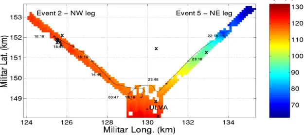
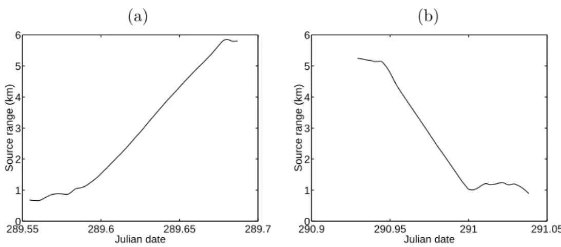
overall description of the sea trial can be found in [8]. This paper concentrates on two events in particular: event II, along a range-independent(RI) track, towards NW from the receiving vertical line array (VLA), and event 5, along a range-dependent(RD) track, to the NE of the VLA. Both events are depicted on figure 1. The bathymetry used for the com-puter model was obtained from direct depth sounding over a 200 m wide path along the acoustic propagation lines, as shown on the colour coded background of figure 1. Figure 2 shows source range versus time as estimated from GPS data, for event 2 (a) and for event 5 (b). The geoacoustic properties were drawn from generic geological knowledge of the area were it was assumed that the NW-RI track had a quite regular bottom, covered by fine sand, and the NE-RD track was largely range-dependent with a background of fine sand and patches of mud, gravel and rock. There were no in situ tests or other acoustic measure-ments in the area previous or after the exper-iment that could be used as additional back-ground information.
2.1 The baseline model
An important first step in tomographic inver-sion is the choice of an environmental model able to represent the mean characteristics of the media where the signal is propagating. Such model will be called the baseline model and generaly includes all the a priori informa-tion available for the problem at hand. In our case there will be two of such models: one for the RI track and the other for the RD track. They basically consist of an ocean layer over-lying a sediment layer and a bottom half space assumed to be range independent. Since for the application at hand little environment in-formation is available all the parameters will be assumed equal for the two models apart from the bathymetry. For a sake of
simplic-ity figure 3 shows the baseline model only for RD-track, knowing that the only differ-ence for the RI-track is that the bathymtery will be constant with a water depth equal to 119 m. For the purpose of inversion the for-ward model parameters were divided into four parameter subsets: geometric, sediment, bot-tom, and water sound speed. The geomet-ric parameters included source range, source depth, receiver depth and bathymetry (in the RD case). The water column sound speed, shown in figure 3, is the mean temperature profile measured at the VLA thermistor sen-sors (see environmental description in [8]).
2.2 Ocean sound speed modelling Another important problem when inverting acoustic data for tomographic purposes, is the difficulty associated with the representation of the sound speed field in time, depth and range, by a finite set of invariant parameters. The classical solution for this problem, known as data regularization, consists on the expan-sion of the temperature, or equivalently the sound speed field1, on a basis of functions rep-resentative of the data set to be estimated. A well known method for obtaining such ba-sis functions, is to calculate the Empirical Orthogonal Functions (EOF) from the eigen-functions of the data correlation matrix. The EOFs were obtained using a singular value de-composition (SVD) of a data matrix C with columns
Ci = ci− ¯c, (1)
where ci are the real profiles available, and ¯c is the average profile. The SVD is known to be
C = UDV, (2)
where D is a diagonal matrix with the singu-lar values, and U is a matrix with orthogonal
columns, which are used as the EOFs. The sound-speed profile is obtained by
CEOF = ¯c +
N
X
n=1
αnUn, (3)
where N is the number of EOFs to be com-bined, judged to accurately represent the sound speed field for the problem at hand. Generally, a criteria based on the total energy contained on the first N EOFs is used. The 14 sound speed profiles obtained from the XBT measurements (see X signs in figure 1) served as database for the computation of the EOFs. The criteria used to select the number of rel-evant EOFs was
ˆ N = min N { PN n=1λ2n PM m=1λ2m > 0.8} (4)
where the λn are the singular values obtained
by the SVD, M is the total number of singu-lar values, provided that λ1 ≥ λ2 ≥ . . . ≥ λM.
For this data set, criteria (4) yielded N = 2, i.e. the first two EOFs are sufficient to model the sound speed with enough accuracy (see figure 4). The coefficients αn, which are the
coefficients of the linear combination of EOFs, are now part of the search space, i.e., they are searched as free parameters.
3
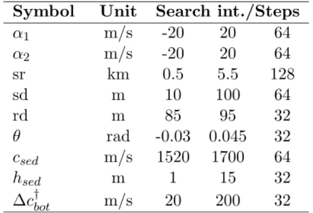
Inversion resultsMultiple environmental and geometrical pa-rameter optimization is often a computation-ally cumbersome task. The first approach to the problem is to try to obtain as much a pri-ori information as possible for the environ-mental parameters in the baseline model, in order to set an interval of variation as narrow as possible into the focalization process. The search intervals for the baseline model des-cribed above have been set according to the values shown in Table 1. The forward compu-tation model used was the normal mode code
CSNAP[9]. The optimization technique for reducing the number of forward computations was based on a genetic algorithm (GA) and the GA implementation used was proposed by Fassbender [10].
Symbol Unit Search int./Steps α1 m/s -20 20 64 α2 m/s -20 20 64 sr km 0.5 5.5 128 sd m 10 100 64 rd m 85 95 32 θ rad -0.03 0.045 32 csed m/s 1520 1700 64 hsed m 1 15 32 ∆c†bot m/s 20 200 32 Table 1: Focalization parameters and search
in-tervals: EOF1 (α1), EOF2 (α2), source range
(sr), source depth (sd), receiver depth (rd), VLA
tilt (θ), compressional sediment speed (csed),
sed-iment thickness (hsed) and bottom compressional
speed variation (∆cbot). † where ∆cbot is assumed
to lay in the interval [ˆcsed+ 20, csed+ 200].
In order to cover a search space of the or-der of 1015, the GA optimizer was set with a population size of 90 individuals and 50 itera-tions. Three independent populations were run for each case. The mutation and the crossover probability were respectively set to 0.008 and 0.7. In particular, a new technique that was found to drastically optimize the search is to use the final solution at a given time point in the initialization of the solving procedure of the next time point.
Let us assume that at time ti the best
in-dividual of the last population is b(ti). The
GA is initialized at time ti+1 such that 30%
of the individuals of the initial population are uniformly distributed within a 10% variation interval of the coordinates of b(ti). The other
70% are randomly distributed in whole search space, as it is usually done, in order to main-tain a high degree of diversity. With this procedure the number of iterations has been
decreased at each time point except for the first one. In practice it is verified that the model fit drops at the begining of each time point when compared with its value at the end of the previous time point, denoting that a misadjustment has been introduced in the data. However, after that initial fitness drop, rapid convergence is obtained leading to pa-rameter values settling down to their ”right” values, or at least those that give the highest fit. The objective function used in this study, was based on the incoherent Bartlett proces-sor in a frequency band selected according to the received signal spectrum.
3.1 The NW-RI track
At the beginning of the run the source was moving away from the VLA location giving the opportunity to test inversion methods with a moving source, which is known to be an always challenging exercise for matched-field algorithms. The source was emitting a series of LFM signals which frequency range, duration and repetition rate is described in [8], and is not repeated here since that infor-mation was neither explicitely or implicitely used in the present study in order to ensure passive tomography constraints. For each time point estimate three consecutive snap-shots were isolated, Fourier transformed and averaged. From the resulting spectra 7 dis-crete frequencies 50 Hz appart in the band 300-600 Hz were extracted for computing the incoherent Bartlett processor.
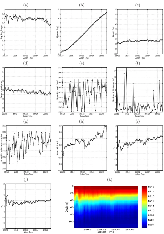
The focalization results are shown in fi-gure 5, plots (a) to (j) and the reconstructed sound speed field is shown in plot (k). These results call for the following comments: first, is that the model fit to the data is excelent with a mean Bartlett power of 0.8, only drop-ping below that value at the end of the run. Source range is perfectly in agreement with the GPS estimated values and, although there
are no complete source depth recordings, the estimated values do agree with cable scope es-timates taking into account ship speed, source weight and cable payout. Note that even the small ship acceleration at the begining of the run is perfectly reproduced with a consequent and logical decrease on the source depth from about 80 to 73 m. Receiver depth and tilt are consistent with the values monitored by the VLA sensors (see report [11]). Bottom properties are consistent with those histori-cally found in that area, that correspond to a thin (2 - 4 m) sediment layer of fine sand or mud, although it may be doubtful that it can be clearly “acoustically seen” at those fre-quencies. The sound speed inversion result shown in plot (k) represents about 2h 15min of data which is clearly a short time interval but denotes a slight rise of the thermocline in agreement with the data observed at the VLA thermistors (see [8]) and in phase with a tidal prediction for that day. Note that during this inversion the source was moving, so the depth-time plot can also be seen as a depth-variable range-average plot, depending if the tempera-ture field is assumed range stationary or time stationary, respectively.
3.2 The NE-RD track
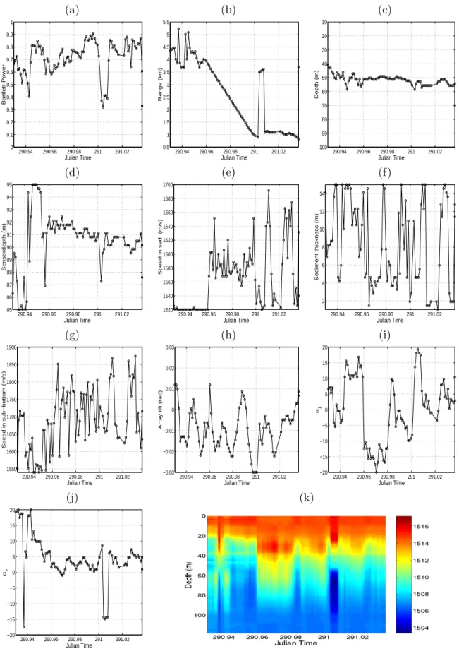
Although a range-independent propagation environment is a view of the reality that al-lows nice theoretical analytical developments, it is, in most cases only a simplified view that does not represent the large majority of the real world situations. In this section the data gathered during event 5, along the NE leg, when the source was at about 5 km range and then approaching the receiver is used to downslope propagate from approximately 70 m water depth to the VLA located in 120 m water depth (see figure 1). This is the most interesting yet, most difficult, case that at-tempts to represent a realistic situation of
an unknwon sound source emitting a PRN sequence at undetermined range and depth, moving over a range dependent environment. The frequency band was the same as that used for the event 2. The results of the inversion are shown in figure 6.
This run is a good example on how the three indicators - source range, source depth and Bartlett power - can be used to validate environmental model estimates. At the be-ginning of the run, until Julian time 290.96, the Bartlett power varies between 0.4 and 0.8, source range changes rapidly and most of the other parameters have highly variable values and some are on, or near, the bounds of their search intervals. So in these initial period, sound speed estimated values are can not be considered as valid. At Julian time 290.96, source range suddenly picks up at 4 km range and steadly follows the approaching of the source to the VLA up to time 291 at about 2 km source range. During that interval most of the parameters, but the EOF coefficient 1, follow stable and credible values well within their respective intervals and are therefore mostly credible. The first EOF coefficient suf-fers a strong, and to date unexplained, change at 290.98 right in the midlle of that smooth path. After Julian time 291, when the source has reached the closest point of approach to the VLA, the “focus” is again suddnely lost with strong variations on all parameters: drop of the Bartlett power from 0.8 to 0.3, a sudden range variation from 1 to 3.5 km and a drop of 10 m on source depth. It was found that time 291 coincides with the low-tide change pro-ducing a 1.5 m rise on the array accompained of strong variations on array tilt, as measured on the depth sensors and tiltmeters on the VLA (see report [11]). The model regains “fo-cus” after 15 min with smooth parameter esti-mates and high Bartlett power values. Among all obtained values within validated intervals
source range and depth were clearly in agree-ment with the expected values, sound speed in the sediment and bottom are reasonably well estimated to have mean values of 1580 and 1700 m/s, with a higher uncertainty in the last one, and finally array depth and array tilt are in good agreement with the pressure and tilt sensors colocated with the VLA. After fo-calization the sound speed evolution through time was reconstructed - plot (k) - showing a highly perturbated estimate due successive focus and lost of focus throughout time.
4
ConclusionsOne of the basic principles of OAT is that both source(s) and receiver(s) are under con-trol - that is, the emitted source signal and the source-receiver geometry is known at all times during the observation window. In passive to-mography the control of the source needs to be relaxed in order to be able to take advan-tage of possible sources of opportunity pass-ing within acoustic range from the receiver(s). Although passive tomography is very appeal-ing for the ease of application, its practical im-plementation is extremely challenging and its full feasibility remains to be proved. BOAT represents a step towards a full demonstration of passive tomography.
This study reports the inversion results obtained on part of the data gathered during the INTIFANTE’00 sea trial, where a towed sound source emitting LFM’s and noise se-quences was used. The challenge is repre-sented by the fact that during the various runs a priori knowledge about the source is progressively relaxed leading to a situation close to that encountered in passive tomo-graphy. In a first data set it was proved that a moving source at an unknown loca-tion emitting a deterministic unknown signal over a range-independent environment can be used for ocean tomography when the
environ-ment and the source position is progressively adapted through time. Estimates of the va-rious environmental and geometrical parame-ters are consistent with expected values. In a second data set the same source was mov-ing towards the array emittmov-ing a PRN signal over a range-dependent environment, repre-senting a scenario close to a possible real pas-sive tomography scenario. It was shown that also in this close-to-real scenario, both geo-metrical and environmental parameters were consistently estimated over time resulting in a high model fit indicating a potential for accu-rate inversion estimates. BOAT was proved to represent the tool of choice for accounting for the unknown geometrical and environmental parameters, inherent to passive tomography feasibility.
Acknowledgments
This work was supported by programe PRAXIS XXI of FCT, Portugal, under projects INTIMATE and ATOMS and under project TOMPACO, CNR, Italy. The authors are also in debt of SACLANTCEN for equip-ment loan and to the crew of NRP D.Carlos I of IH, that made the sea trial successful.
References
[1] Collins M.D. and Kuperman W.A. Fo-calization: Environmental focusing and source localization. J. Acoust. Soc. America, 90(3):1410–1422, September 1991.
[2] P. Gerstoft and D. Gingras. Parameter estimation using multi-frequency range-dependent acoustic data in shallow wa-ter. J. Acoust. Soc. America, 99(5):2839– 2850, 1996.
[3] P. Gerstoft. Inversion of seismoacous-tic data using geneseismoacous-tic algorithms and a
posteriori probability distributions. J. Acoust. Soc. America, 95(2):770–782, 1994.
[4] Hermand J.-P. and Gerstoft P. Inversion of broad-band multitone acoustic data from the yellow shark summer experi-ments. IEEE Journal pf Oceanic Engi-neering, 21(4):324–364, 1996.
[5] Soares C., Waldhorst A., and Jesus S. Matched field processing: Environmen-tal focusing and source tracking with ap-plication to the north elba data set. In Proc. of the Oceans’99 MTS/IEEE con-ference, pages 1598–1602, Seattle, Wash-ington, 13-16 September 1999.
[6] Soares C.J., Siderius M., and Jesus S.M. Matched-field source localization in the strait of sicily. accepted to J. Acoust. Soc. America, July 2001.
[7] Soares C., Siderius M., and Jesus S. High frequency source localization in the strait of sicily. In Proc. of the MTS/IEEE
Oceans 2001, Honolulu, Hawai, USA, 5-8 November 2001.
[8] Jesus S., Coelho E., Onofre J, Picco P, Soares C., and Lopes C. The intifante’00 sea trial: preliminary source localization and ocean tomography data analysis. In Proc. of the MTS/IEEE Oceans 2001, Honolulu, Hawai, USA, 5-8 November 2001.
[9] C. M. Ferla, M. B. Porter, and F. B. Jensen. C-SNAP: Coupled SACLANT-CEN normal mode propagation loss model. La Spezia, Italy.
[10] T. Fassbender. Erweiterte genetische algorithmen zur globalen optimierung multimodaler funktionen. Diplomarbeit, Ruhr-Universit¨at Bochum, 1995.
[11] Jesus S., Silva A., and Soares C. In-tifante’00 sea trial data report - events i, ii and iii. Internal Report Rep. 02/01, SiPLAB/CINTAL, Universidade do Al-garve, Faro, Portugal, May 2001.
Figure 1: INTIFANTE’00 sea trial site bathymetry with XBT locations (marked×) and acoustic tracks for events 2 and 5.
(a) (b) 289.550 289.6 289.65 289.7 1 2 3 4 5 6 Julian date Source range (km) 290.90 290.95 291 291.05 1 2 3 4 5 6 Julian date Source range (km)
Figure 2: Source - VLA receiver range vs. time for the NW-RI track (a) and the NE-RD track (b). 0 60 119 Depth (m) Range (km) Source (63 m) Subbottom 0 2 5.7 1506 1518 m/s α=0.8 dB/λ ρ=1.9 g/cm3 1800 m/s VA Sediment 2.0 m 1650 m/s α =0.8 dB/λ ρ=1.9 g/cm3
Figure 3: Baseline environmental model for the NE range-dependent track.
(a) (b) 1506 1510 1515 0 20 40 60 80 100 119 Soundspeed (m/s) Depth (m) −0.2 −0.1 0 0.1 0 20 40 60 80 100 119 Soundspeed (m/s) Depth (m) 1st EOF 2nd EOF
Figure 4: XBT based data used for ocean sound speed estimation: mean sound speed profile (a) and empirical orthonormal functions (EOFs) (b).
(a) (b) (c) 289.580 289.6 289.62 289.64 289.66 0.1 0.2 0.3 0.4 0.5 0.6 0.7 0.8 0.9 1 Julian Time Bartlett Power 289.58 289.6 289.62 289.64 289.66 0.5 1 1.5 2 2.5 3 3.5 4 4.5 5 5.5 Julian Time Range (km) 289.58 289.6 289.62 289.64 289.66 10 20 30 40 50 60 70 80 90 100 Julian Time Depth (m) (d) (e) (f) 289.5885 289.6 289.62 289.64 289.66 86 87 88 89 90 91 92 93 94 95 Julian Time Sensordepth (m) 289.58 289.6 289.62 289.64 289.66 1520 1540 1560 1580 1600 1620 1640 1660 1680 1700 Julian Time Speed in sed. (m/s) 289.58 289.6 289.62 289.64 289.66 2 4 6 8 10 12 14 Julian Time Sediment thickness (m) (g) (h) (i) 289.58 289.6 289.62 289.64 289.66 1550 1600 1650 1700 1750 1800 1850 1900 Julian Time Speed in sub−bottom (m/s) 289.58 289.6 289.62 289.64 289.66 −0.03 −0.02 −0.01 0 0.01 0.02 0.03 0.04 Julian Time
Array tilt (rad)
289.58 289.6 289.62 289.64 289.66 −20 −15 −10 −5 0 5 10 15 20 Julian Time α1 (j) (k) 289.58 289.6 289.62 289.64 289.66 −20 −15 −10 −5 0 5 10 15 20 Julian Time α2
Figure 5: Focalization results for Event 2: Bartlett power (a), source range (b), source depth (c), receiver depth (d), sediment compressional speed (e), sediment thickness (f ), sub-bottom com-pressional speed (g), VLA tilt (h), EOF coefficient 1 (i), EOF coefficient 2 (j) and reconstructed sound speed (k).
(a) (b) (c) 290.94 290.96 290.98 291 291.02 0 0.1 0.2 0.3 0.4 0.5 0.6 0.7 0.8 0.9 1 Julian Time Bartlett Power 290.94 290.96 290.98 291 291.02 0.5 1 1.5 2 2.5 3 3.5 4 4.5 5 5.5 Julian Time Range (km) 290.94 290.96 290.98 291 291.02 10 20 30 40 50 60 70 80 90 100 Julian Time Depth (m) (d) (e) (f) 290.94 290.96 290.98 291 291.02 85 86 87 88 89 90 91 92 93 94 95 Julian Time Sensordepth (m) 290.94 290.96 290.98 291 291.02 1520 1540 1560 1580 1600 1620 1640 1660 1680 1700 Julian Time Speed in sed. (m/s) 290.94 290.96 290.98 291 291.02 2 4 6 8 10 12 14 Julian Time Sediment thickness (m) (g) (h) (i) 290.94 290.96 290.98 291 291.02 1550 1600 1650 1700 1750 1800 1850 1900 Julian Time Speed in sub−bottom (m/s) 290.94 290.96 290.98 291 291.02 −0.03 −0.02 −0.01 0 0.01 0.02 0.03 Julian Time
Array tilt (rad)
290.94 290.96 290.98 291 291.02 −20 −15 −10 −5 0 5 10 15 20 Julian Time α1 (j) (k) 290.94 290.96 290.98 291 291.02 −20 −15 −10 −5 0 5 10 15 20 Julian Time α2
Figure 6: Focalization results for Event 5: Bartlett power (a), source range (b), source depth (c), receiver depth (d), sediment compressional speed (e), sediment thickness (f ), sub-bottom com-pressional speed (g), VLA tilt (h), EOF coefficient 1 (i), EOF coefficient 2 (j) and reconstructed sound speed (k).