Assessment of reserve effect in a marine protected area: the case study of the Professor Luiz Saldanha Marine Park (Portugal)

Faculdade de Ciências e Tecnologia

Assessment of reserve effect in a Marine

Protected Area: the case study of

the Professor Luiz Saldanha

Marine Park (Portugal)

Inês Isabel Gralho Correia de Sousa

Faculdade de Ciências e Tecnologia

Assessment of reserve effect in a Marine Protected

Area: the case study of the Professor Luiz Saldanha

Marine Park (Portugal)

Thesis developed within the LIFE-BIOMARES project (LIFE06 NAT/ P/000192)

Dissertation submitted in fulfillment of the requirements for the Degree of Master in Marine Biology – specialization in Marine Ecology and Conservation

“For most of history, man has had to fight nature to survive. In this century he is beginning to realize that, in order to survive, he must protect it.” Jacques-Yves Cousteau

I hereby declare that I am the sole author of this thesis Esta dissertação é da exclusiva responsabilidade da autora

i Many persons contributed to make the present work possible, and to whom I would like to thank:

To Professor Doctor Karim Erzini, whose supervision was essential to develop this thesis and to undertake the research work in the Life-Biomares project.

To Professor Doctor Jorge Gonçalves, whose supervision and advices where crucial to develop this thesis.

To Dr. Alexandra Cunha, for the coordination and support in the Life-Biomares project.

To Dr. Rui Coelho and Dr. Rita Costa Abecasis, for all the quality work undertaken in the Life-Biomares project, and that enabled the development of this thesis.

To Mestre Joaquim M. Silva, for his availability and good will in undertaking the field work onboard his vessel.

To all the good willing colleagues at the Life-Biomares project that helped me on field surveys: Francisco Pires, Diogo Paulo, Joana Boavida, Sandra Rodrigues, Vasco Ferreira, and Marina Mendes.

To all the colleagues and volunteers who helped in sampling surveys: Marie Renwart, Joana Barosa, Sarah Laura Simons, David Abecasis, Joana Dias, Vera Viegas, Tim Puts, Elisabeth Debusschere, and Bogdan Glogovac.

To all the colleagues and friends at the Coastal Fisheries Research Group: Mafalda Rangel, Laura Leite, Frederico Oliveira, Pedro Monteiro, Pedro Veiga, Isidoro Costa, Carlos Afonso, and Luís Bentes. Thank you for the friendship and support.

To Mafalda Rangel, whose support was precious at the final stage of this thesis.

To Luís Bentes, Pedro Monteiro, Pedro Veiga, and Laura Leite, for all the precious advices, specifically regarding statistics.

ii To Pedro Decq Mota, for his unconditional support, precious advices and availability at any time of the day. For believing in me. To him, I leave a very special thanks.

iii (Arrábida coast), comprising 38 km of coastline. It was established in 1998 and in August 2005 specific management measures were implemented. Three protection levels were established: Total – human activities not allowed; Partial - some fishing allowed with some gears (octopus traps, jigging, handline); Complementary - fishing allowed with vessels under 7m length and licensed to operate within the marine park. To monitor the reserve effect, in terms of abundance, biomass and also community composition, experimental fishing trials with trammel nets on soft bottoms have been conducted since 2007 (depths between 10 – 45m). The individuals caught were identified to species level, measured to the nearest mm and released when alive. The data (species abundance and biomass) were analyzed both with univariate and multivariate methods, allowing the comparison between the three protection levels.

The data analysis showed higher values of Catch per Unit Effort (CPUE) in number and in weight for the Partial and Total protection areas when compared to the Complementary, where fishing with nets is allowed. Also the biodiversity indices (Margalef and Shannon-Wiener) showed higher values in these two areas. The multivariate analysis (ANOSIM) supports the previous results, in the sense that the communities from Partial and Total sections were found to be significantly different from the one found in the Complementary area. The SIMPER analysis showed that the bastard sole Microchirus azevia and the toadfish Halobatrachus didactylus are important contributors for the distinction of these communities. It was noticed that in assessing the reserve effect, the benefits of protection is differed from species to species. The analysis at the species level was important in the detection of trends that are probably related with the implemented protection measures. Namely the species Chelidonichthys lucerna, M. azevia and Raja clavata showed abundance increases from the first analyzed period (Aug. 2007 - Aug. 2009) to the second (Aug. 2009 - Aug. 2010), after the full implementation of the marine park. Besides the increase in abundance, C. lucerna and M. azevia also registered an increase in the median total length. Overall, the results suggest that the Partial and Total protection areas are important for several soft bottom species. The importance of protection level was confirmed by Gaussian GAM models, for both sandy and muddy bottom. This analysis also revealed water temperature as an important predictor of CPUE in weight.

The results obtained include the first signs of a reserve effect concerning the soft bottoms of the Prof. Luiz Saldanha Marine Park. The protection measures, mainly the restriction on the use of trammel and gill nets, seem to benefit some bottom associated species. To better understand the reserve effect on the biodiversity and abundance of soft bottom communities, further sampling should be considered.

iv Arrábida) e inclui 38 km de litoral. Este parque foi estabelecido em 1998 e em Agosto de 2005 foram implementadas medidas de gestão específicas. Três estatutos de protecção foram estabelecidos: Total – interdição total às actividades humanas; Parcial - alguma pesca permitida com determinadas artes de pesca (covos, toneira, linha de mão); Complementar - pesca permitida a barcos até aos 7m e licenciados para operar dentro do parque marinho. A fim de monitorizar o efeito de reserva em termos de abundância, biomassa e composição da comunidade, desde 2007 que se têm realizado campanhas de pesca experimental com rede de tresmalho (profundidade entre 10 – 45m) sobre substratos móveis. Os indivíduos capturados foram identificados até ao nível da espécie, medidos ao mm mais próximo e libertados quando vivos. Os dados (abundância e biomassa por espécie) foram analisados com métodos univariados e multivariados, permitindo a comparação dos três estatutos de protecção.

Foram obtidos valores de Captura por Unidade de Esforço (CPUE) em número e em peso mais elevados nas áreas de protecção Parcial e Total do que na Complementar, onde a pesca com redes é permitida. Também os índices de biodiversidade (Margalef e Shannon-Wiener) revelaram valores mais elevados nestes duas áreas. A análise multivariada (ANOSIM) suporta os resultados referidos, uma vez que se verificaram diferenças significativas entre as comunidades das secções Parcial e Total em comparação com a encontrada na Complementar. A análise SIMPER mostrou que as espécies Microchirus azevia e Halobatrachus didactylus contribuem de forma importante para a distinção destas comunidades. Os resultados estão de acordo com o facto de que a vantagem derivada das medidas de protecção difere de acordo com a espécie. A análise ao nível das espécies foi útil na detecção de tendências que estão provavelmente relacionadas com as medidas de protecção implementadas. Nomeadamente, as espécies Chelidonichthys lucerna, M. azevia e Raja clavata, mostraram aumentos de abundância entre o primeiro (Agosto 2007 - Agosto 2009) e o segundo (2009 de agosto - 2010 de agosto) período analisado. Além do aumento em abundância, as espécies C. lucerna e M. azevia também registaram um aumento no comprimento total médio. De um modo geral, os resultados sugerem que as áreas de protecção Parcial e Total são importantes para várias espécies de substratos móveis. A importância do nível de protecção foi confirmada nos modelos GAM de distribuição gaussiana obtidos para os substratos arenoso e lodoso. Esta análise também revelou a temperatura da água como um factor importante na previsão do peso da captura.

Os resultados obtidos parecem incluir os primeiros sinais do efeito de reserva nos substratos móveis do Parque Marinho Professor Luiz Saldanha. As medidas de protecção, principalmente a restrição do uso de redes de tresmalho e emalhar, parecem beneficiar as espécies que vivem associadas ao fundo. Para analisar devidamente o efeito de reserva na biodiversidade e abundância das comunidades de substratos móveis, é aconselhada a continuação da amostragem.

v

Abstract ... iii

Resumo ... iv 1. Introduction ... 1

1.1. Study area ... 2

2. Material and Methods... 6

2.1. Sampling method ... 6

2.2. Data treatment ... 9

2.2.1. Quantitative analysis ... 10

2.2.2. Diversity analysis ... 11

2.2.3. Spatial and temporal analysis ... 11

2.2.4. Multivariate analysis ... 13 2.2.5. Model fitting ... 14 3. Results ... 17 3.1. Sample representativity ... 17 3.2. Temperature analysis ... 18 3.3. Biological parameters ... 18

3.4. Analysis of catch data ... 22

3.4.1. Species trends ... 27

3.5. Multivariate analysis ... 33

3.6. Model fitting ... 37

4. Discussion ... 46

4.1. Analysis of catch data ... 46

4.2. Model fitting ... 51

4.3. Final considerations ... 53

5. References ... 55 ANNEXES

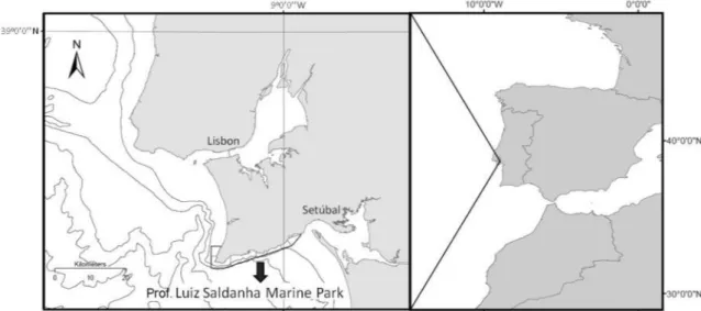
vi Figure 1. Location of the Prof. Luiz Saldanha Marine Park (PLSMP) on the west coast of Portugal. ... 3

Figure 2. The Prof. Luiz Saldanha Marine Park (PLSMP) and its three different protection levels. The five different sections that compose the experimental trammel nets sampling area are shown (A, B, C, D and E). Each section undertook a different evolution during the implementation period (January 2006 – August 2009; See Annex I). ... 4

Figure 3. The Prof. Luiz Saldanha Marine Park (PLSMP) map with respective protection area delimitations and the location of the experimental trammel net sets. ... 8

Figure 4. Map of the sampling area in the Prof. Luiz Saldanha Marine Park. All the sampling points (middle point of each 500m long net set) are shown (red dots). ... 9

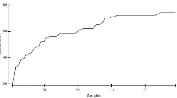
Figure 5. Species accumulation curve in relation to the cumulative number of samples (trammel net sets). ... 17

Figure 6. Boxplot of temperature (measurements during spring and autumn sampling campaigns) by period (Years 3-4: Aug. 2007 - Aug. 2009; Year 5: Aug. 2009 - Aug. 2010). ... 18

Figure 7. Boxplot of the Margalef and Shannon-Wiener indeces by protection level and by period (Years 3-4: Aug. 2007 - Aug. 2009; Year 5: Aug. 2009 - Aug. 2010). ... 22

Figure 8. Boxplots of the CPUE in weight (Kg.1000m-1) (A), CPUE in number (number.1000m-1) (B) and catch value (€.1000m-1

) (C) by protection level and by period (Years 3-4: Aug. 2007 - Aug. 2009; Year 5: Aug. 2009 - Aug. 2010). ... 24

Figure 9. Boxplots of the specimens total length (cm) (A), weight (g) (B) and estimated value (€) (C) by protection level and by period (Years 3-4: Aug. 2007 - Aug. 2009; Year 5: Aug. 2009 - Aug. 2010). ... 25

Figure 10. Boxplot of the CPUE in weight (Kg.1000m-1) by sector and by period (Years 3-4: Aug. 2007 - Aug. 2009; Year 5: Aug. 2009 - Aug. 2010). ... 26

Figure 11. Boxplots of the specimens total length (cm) by protection level and by period (Years 3-4: Aug. 2007 - Aug. 2009; Year 5: Aug. 2009 - Aug. 2010). Data for four bony fish species: Chelidonichthys lucerna (A), Microchirus azevia (B), Solea senegalensis (C) and Solea solea (D). ... 28

vii species: Chelidonichthys lucerna (A), Microchirus azevia (B), Solea senegalensis (C) and Solea solea (D). ... 30

Figure 13. Boxplots of the CPUE in number (number.1000m-1) by protection level and by period (Years 3-4: Aug. 2007 - Aug. 2009; Year 5: Aug. 2009 - Aug. 2010). Data for four elasmobranch taxa: Torpedo torpedo (A), Myliobatis aquila (B), Raja clavata (C) and family Rajidae (D). ... 31

Figure 14. NMDS ordination of samples based on Bray-Curtis similarity (4th root data transformation). Samples are labeled according to protection level. ... 34

Figure 15. Contribution of analyzed variables (when applied as the only predictor) in explaining the variance of CPUE in weight. Model fitting: Gaussian GAM, identity link function. ... 37

Figure 16. Estimated smoothing curves for water temperature (A) and depth (B) in the sandy bottom model. The solid line is the smoother and the dotted lines are 95% point-wise confidence bands. ... 42

Figure 17. Estimated smoothing curve for water temperature in the muddy bottom model. The solid line is the smoother and the dotted lines are 95% point-wise confidence bands. ... 42

Figure 18. Sandy bottom model - Model validation through graphical analysis of the residuals. A - Q-Q plot; B - Residuals versus linear predictor; C - Histogram of the residuals; D - Response against fitted values. ... 44

Figure 19. Sandy bottom model - Residuals obtained by the fitted GAM model plotted versus their spatial coordinates. Black dotes are negative residuals, and grey dots are positive residuals. Size of dots is proportional to value. ... 44

Figure 20. Muddy bottom model - Model validation through graphical analysis of the residuals. A - Q-Q plot; B - Residuals versus linear predictor; C - Histogram of the residuals; D - Response against fitted values. ... 45

Figure 21. Muddy bottom model - Residuals obtained by the fitted GAM model plotted versus their spatial coordinates. Black dotes are negative residuals, and grey dots are positive residuals. Size of dots is proportional to value. ... 45

viii Table I. Regulations implemented (Ministers Council Resolution No. 141/2005, 23rd August 2005) in the Prof. Luiz Saldanha Marine Park regarding commercial fishing. ... 5

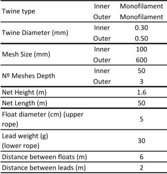
Table II. Specifications of the trammel nets used during the scientific surveys. ... 6

Table III. Characteristics of the sites sampled during the experimental trammel nets surveys. ... 8

Table IV. List of variables considered for model fitting and their characteristics. ... 16

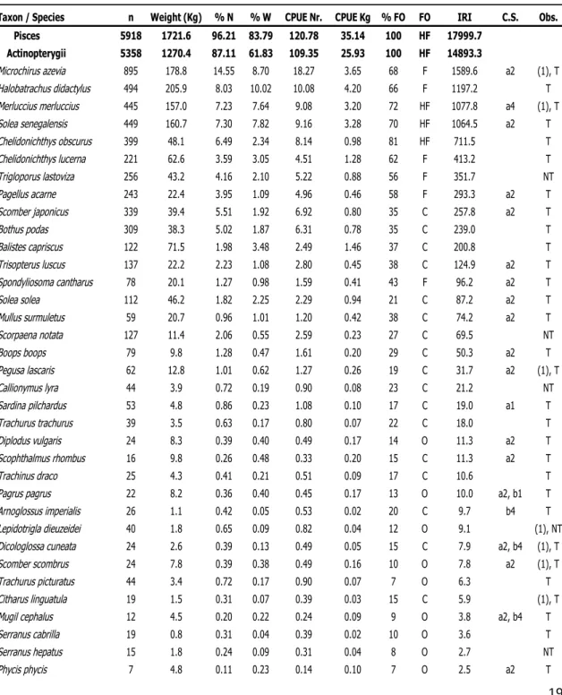
Table V. Commercial fish and invertebrate species caught in the trammel net surveys (FO: frequency of occurrence; IRI: index of relative importance; C.S.: conservation status). Species ordered by IRI. ... 19

Table VI. CPUE and frequency of occurrence (FO) of the invertebrates with no commercial value. ... 21

Table VII. Results of the Kruskal-Wallis One-Way ANOVA on Ranks (α=0.05) applied to the Margalef and Shannon-Wiener indeces for each protection level and in each period. ... 22

Table VIII. Results of the Kruskal-Wallis One-Way ANOVA on Ranks (α=0.05) applied to compare values according to protection level and period - CPUE (ind.1000m-1 and Kg.1000m-1), catch value (€); values per individual: total length (TL), mean weight and mean value. ... 26

Table IX. Results of the Kruskal-Wallis One-Way ANOVA on Ranks (α=0.05) applied to CPUE in weight (Kg.1000m-1) obtained for each sector (Complementary; Partial West, Total, Partial East) and in each period. ... 27

Table X. Results of Kruskal-Wallis One-Way ANOVA on Ranks (α=0.05) to compare the median total length (TL) of four bony fish species according to protection level and period. ... 29

Table XI. Results of Kruskal-Wallis One-Way ANOVA on Ranks (α=0.05) applied to eight fish species, comparing the CPUE in number (ind./1000m) per protection level and period. ... 32

Table XII. Results of one-way ANOSIM (α=0.01; 4th

root data transformation; Bray-Curtis similarity) according to protection level; all samples included (Global R=0.252). ... 33

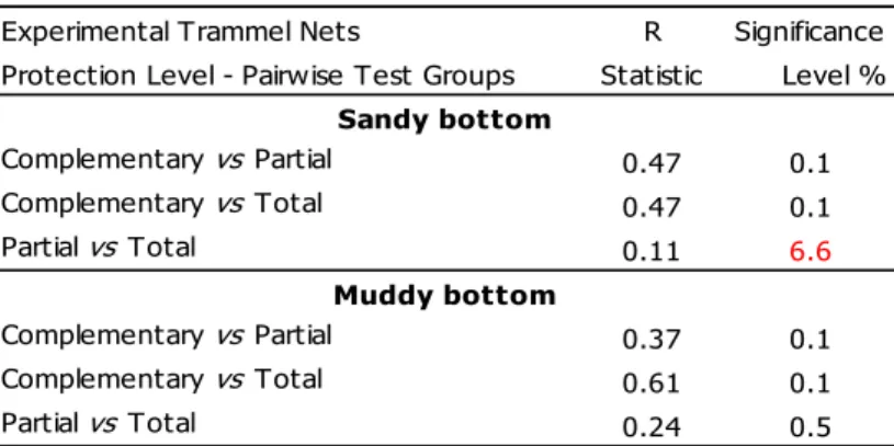
ix samples separately (Global R „sandy bottom‟ = 0.343; Global R „muddy bottom‟ = 0.368)... 34

Table XIV. SIMPER results for the protection level comparisons (4th root data transformation; Bray-Curtis similarity); all samples included. Species with Contribution% ≥ 3.5 are shown. ... 36

Table XV. SIMPER results for substrate/depth comparisons: sandy (10-18m depth) and muddy bottoms (35-40m depth) (4th root data transformation; Bray-Curtis similarity). Species with Contribution% ≥ 3.5 are shown. ... 36

Table XVI. Forward stepwise procedure applied in the GAM model fitting for both substrate groups: sandy and muddy bottoms. ... 39

Table XVII. Parameters estimated for the GAM fitted with the sandy bottom samples. ... 39

Table XVIII. Parameters estimated for the GAM fitted with the muddy bottom samples. ... 40

Table XIX. Null deviance, residual deviance, explained deviance, AIC and degrees of freedom obtained for each model: sandy and muddy bottom. ... 41

x Annex I. Illustration of the Prof. Luiz Saldanha Marine Park (PLSMP) implementation period

applied to commercial fishing. ... i

Annex II. Details of the experimental trammel nets sampling campaigns. ... ii

Annex III. Field operations undertaken during the experimental trammel nets campaigns. ... iii

Annex IV. List of all the variables used during data exploration. ... iv

Annex V. Details of the additional campaigns with trammel nets used in model fitting. ... v

Annex VI. Data exploration undertaken previously to model fitting. ... vi

Annex VII. R code used for model fitting. ... xi

Annex VIII. Data exploration of the variable „Temperature‟. Results of the Mann Whitney Rank Sum tests for temperature per period and season. ... xii

Annex IX. Contribution of each taxon to the total number of individuals caught in the Prof. Luiz Saldanha Marine Park (PLSMP) area and according to protection level. ... xiv

Annex X. Some specimens caught during the experimental trammel nets campaigns. ... xv

Annex XI. Results of the Dunn pairwise comparisons for the Margalef and Shannon-Wiener diversity indeces. ... xvi

Annex XII. Results of the Dunn pairwise comparisons for the variables CPUE in number, CPUE in weight, Catch Value, Total length, Weight per individual and Value per individual. ... xvii

Annex XIII. Results of the Dunn pairwise comparisons for CPUE in weight according to sector and period. ... xix

Annex XIV. Exploratory data analysis of the CPUE in weight. ... xx

Annex XV. CPUE in number and in weight per species and per sector. ... xxiv

Annex XVI. Results of the Dunn pairwise comparisons for the total length of four bony fish species. ... xxvii

xi Annex XVIII. Graphical analysis for comparison of the CPUE in weight of eight fish species in the Partial and Total protection areas versus the Complementary area. ... xxx

Annex IX. Results of the SIMPER analysis for the sandy and muddy bottom samples and according to the protection level... xxxi

1

1. Introduction

The marine environment provides diverse and valuable resources, while at the same time enabling essential environmental functions and processes to take place. For centuries, oceans were regarded as providers of limitless and openly accessible resources and exploitation occurred with little regard for sustainability. Many marine ecosystems are nowadays heavily impacted by human activities. Fisheries relying on high trophic level species have been reported worldwide as undergoing striking declines due to exploitation (Pauly et al., 1998; Pauly and Palomares, 2005). Moreover, 80 percent of the world fish stocks for which assessment information is available are currently overexploited or fully exploited (FAO, 2009). Several policies that led to mismanagement over the years are beyond this fisheries global crisis (Pauly et al., 2002). For instance, the single-species stock assessment has failed in the management of cod given that it grossly underestimated the severity of the population decline and the increasing impacts of fishing during the decline (Walters and Maguire, 1996). Resulting changes in ecological structure coupled with global climate changes and other impacts lead to increasingly less ability of the marine ecosystems to support demand, even as demand continues to increase (Agardy, 2000).

Marine protected areas (MPAs) are increasingly being chosen from the variety of options available to managers, largely because conventional measures have repeatedly failed (Agardy, 1994, Walters and Maguire, 1996). Classical management, based on capture rates and fishing effort relies on large quantities of information and its application to multi-species fisheries is limited (Roberts and Polunin, 1991). Increasingly, marine reserves are being suggested as an appropriate tool to use side by side with classical practices (Pauly et al., 2002; Russ, 2002). Creating a reserve and decreasing the effort are two different strategies that should be engaged to deal with the large uncertainty associated with fisheries management (Clark, 1996; Pauly et al., 2002). Enclosing areas from exploitation diminishes our dependence on precise and real-time information, due to the protection of part of the population from overharvesting (Botsford et al., 1997; Pauly et al., 2002).

Besides the consumptive values of living resources, non-consumptive values are also generated by marine protected areas (Carter, 2003). In addition to consumptive uses, which include commercial and recreational fishing among other harvesting activities, non-extractive uses of the resources are instigated, such as recreational diving, research activities and the protection of nursery grounds (Greenville, 2007).

Few studies have focused on the economic costs and benefits of MPAs. Nevertheless, the majority conclude that under the appropriate conditions, these areas bring benefits that justify their implementation (Alder et al., 2002). Some authors defend that it is not wise to assume that local effects due to marine reserves have consequences on population dynamics on a wide scale and stock predictions based on this should be avoided (Willis et al., 2003b). Nevertheless, it is acknowledged that the local protection of resources has the potential to improve species

2 resilience and several studies have already shown evidences that these measures can bring benefits to fisheries through the migration of adults, juveniles and larvae (Gell and Roberts, 2003).

Marine protected areas are nowadays one of the most promising solutions to meet conservation and fisheries management in coastal areas, and are being implemented worldwide, not only in areas known as biodiversity „hotspots‟, like coral reefs (Schmidt, 1997; Allison et al., 1998), but also in temperate areas, particularly in coastal zones that are vulnerable to human pressure, which is the case of many protected areas in the Mediterranean (Limousin, 1995; Nogueira and Romero, 1995).

In Portugal, the use of marine protected areas as tools to conservation and management is still considered an innovative approach, as only a few marine parks have been implemented, most of them in the Azores (Santos et al., 1995). In mainland Portugal, the Prof. Luiz Saldanha Marine Park (PLSMP) was one of the first marine protected areas. Its main objective is the conservation of coastal biodiversity, although it is also intend to be a tool for fisheries management (Gonçalves et al., 2003).

Scientific research that took place in this coastal region revealed that is an area with particularly high biodiversity. Henriques et al. (1999) obtained results on the local fish assemblages that revealed a level of biodiversity that is remarkably high when compared to the values reported for similar latitudes in the north-eastern Atlantic and the Mediterranean. Moreover this area is known to provide representative habitats for a high proportion of the total shallow-water fish and invertebrate fauna of the Portuguese mainland shores. These facts emphasize the extreme importance of conservation measures in this region (Henriques et al., 1999; Gonçalves et al., 2003).

The aim of the present work was to assess the effects of the Prof. Luiz Saldanha Marine Park management measures on the marine community. For this, a qualitative and quantitative assessment of the fauna occurring on soft bottoms under different protection levels was undertaken through trammel net experimental fishing. Given the recent implementation of this marine park, it was even more fundamental to obtain scientific information concerning the changes occurring in the marine community.

1.1. Study area

Located in western Portugal, the Arrábida coast is recognized for its ecological importance and high marine biodiversity (Henriques et al., 1999; Gonçalves et al., 2003). Protected from the dominant northern winds, the coastline is characterized by high rocky cliffs alternated by sheltered bays (Ribeiro, 2004). In most of the area under 15 - 20 m deep, the rocky bottoms are replaced by soft bottoms.

3 The coastal section from Portinho da Arrábida to the Sesimbra bay is characterized by a narrow rocky band that extents to a maximum of 20 m deep. The rocky substrate is delimited by sandy bottoms that can go up to 100 m deep in the adjacent area of the marine park. Protected bays with intertidal boulders as well as sand banks are also found in this region. From the Sesimbra bay to west, besides the shallow rocky bottom and sandy areas, patches of subsurface rock can also be found (Gonçalves et al., 2003).

This diversity of habitats gives place to more than 1000 species of marine fauna and flora already described for the region (Saldanha, 1974; Calado and Gaspar, 1995; Henriques et al., 1999; Almada et al., 2000; Gonçalves et al., 2003).

It is worth pointing out that this coast is located near the large metropolitan area of Lisbon, which makes it highly susceptible to intense pressures from leisure and economic activities. Some of these human activities such as fisheries and tourism, have high local importance, both socially and economically (Gonçalves et al., 2003).

The need to couple the area usage with conservation and management concerns led to the conception of legal regulation, with the establishment of the Professor Luiz Saldanha Marine Park (PLSMP; also known as „Arrábida Marine Park‟) in 1998. Its implementation aims to protect coastal ecosystems and also promote the sustainability of fisheries resources (Gonçalves et al., 2003; Reis et al., 2004). This marine protected area is included in the Arrábida Natural Park and comprises an area with 52 km2, which stretches over 38 km of coast and reaches depths up to 100 meters (Figure 1).

Figure 1. Location of the Prof. Luiz Saldanha Marine Park (PLSMP) on the west coast of Portugal.

It was only in August 2005 that the usage of the PLSMP area was regulated. The official legislation of the Ministers Council Resolution No. 141/2005, 23rd August 2005, divided the region in three different protection areas – Complementary, Partial and Total (Figure 2) – which differ in the level of restrictions imposed. The main restrictions of each area are: Total – human

4 activities not allowed; Partial – some fishing allowed with some gears (octopus traps, jigging, handline); Complementary – fishing allowed but restricted to vessels under 7m length and licensed to operate within the marine park (Resolução do Conselho de Ministros, 2005). The complete descriptions of each area and its restrictions concerning commercial fishing are given in Table I. In relation to recreational fishing, angling is only permitted in the Complementary area and spearfishing is prohibited in all the marine park area. The establishment of this regulation attempts to harmonize, on the one hand, the region‟s biodiversity and ecological importance, and on the other, the important socio-economical activities that take place there. The restrictions related to commercial fishing were implemented gradually during the period between 2006 to 2009: after the establishment of the Complementary protection level in all the marine park area in January 2006, two areas with Partial protection were implemented in August 2006, and in August 2007 four more were created. In August 2008, one Partial protection area was upgraded to Total protection. The last implementation step occurred in August 2009, with enlargement of the previous Total protection area. A detailed illustration of each implementation step is shown in the Annex I.

Figure 2. The Prof. Luiz Saldanha Marine Park (PLSMP) and its three different protection levels. The five different sections that compose the experimental trammel nets sampling area are shown (A, B, C, D and E). Each section undertook a different evolution during the implementation period (January 2006 – August 2009; See Annex I).

5 Table I. Regulations implemented (Ministers Council Resolution No. 141/2005, 23rd August 2005) in the Prof. Luiz Saldanha Marine Park regarding commercial fishing.

Area Fishing Gear Management Regulations

Fishing allowed only to boats under 7m length and licensed to operate within the marine park Purse seine Not allowed

Trawling Not allowed Handline and Jigging Allowed

Octopus Traps Allowed (minimum distance from shore line: 200 m) Longline Allowed

Trammel and Gill nets Allowed (minimum distance from shore line: 1/4 nm) Handline and Jigging Allowed (minimum distance from shore line: 200 m)

Octopus Traps Allowed (minimum distance from shore line: 200 m) Longline Not allowed

Trammel and Gill nets Not allowed

Total Human activities not allowed

Protection Area Boats are only allowed to navigate at more than 1/4 nm from shore line

All All All PLSMP Area Complementary Protection Area Partial Protection Area

6

2. Material and Methods

2.1. Sampling method

The data for this study was obtained during the course of the LIFE-BIOMARES Project (LIFE06 NAT/ P/000192). This project was funded by the European Commission Program LIFE-Nature, with co-financing from SECIL Company (Companhia Geral de Cal e Cimento S.A.).

Since 2007, CCMAR (Centre of Marine Sciences, Algarve) researchers involved in Task D5 (fisheries indicators monitoring) of the LIFE-BIOMARES project have been carrying out experimental fishing surveys on a seasonal basis in the PLSMP area. The sampling has been taking place in the three different PLSMP protection levels, on both sandy and muddy bottoms. The experimental fishing gear used consisted of a trammel net similar to the type used by the local fishermen (Sesimbra), and for this purpose a local fisherman was contracted to make the trammel nets. The experimental net was made of monofilament and consisted of an inner mesh panel with 100mm stretched mesh and two outer panels with 600mm stretched mesh. The inner net monofilament mesh is of 0.30mm in diameter while that of the outer net is 0.50mm. The net was constructed to have 50 inner and 3 outer meshes in height, with a total height of 1.60m.

Table II. Specifications of the trammel nets used during the scientific surveys. Inner Monofilament Outer Monofilament Inner 0.30 Outer 0.50 Inner 100 Outer 600 Inner 50 Outer 3 Net Height (m) 1.6 Net Length (m) 50

Float diameter (cm) (upper

rope) 5

Lead weight (g)

(lower rope) 30

Distance between floats (m) 6

Distance between leads (m) 2

Twine type

Mesh Size (mm) Nº Meshes Depth Twine Diameter (mm)

7 Each net had a total of 50m in length and each set consisted of 10 nets. At each location, monitoring was carried out with one set, consisting of a total of 500m of trammel net. Normal fishing practices were followed, leaving the Sesimbra fishing harbour before dawn on board of a typical local fishing boat prepared to operate with trammel nets (fibre glass boat with pilot house; overall length: 6.98m). The nets were set around noon and hauling took place early in the morning just after sunrise. The soak time varied between 20 to 24 hours. This standardized fishing procedure enables Catch per Unit Effort (CPUE) – to be defined by a unit effort of 500m of trammel net, and a soak time of approximately 24 hours. The position of each set was tracked with a handheld Garmin 60CSx GPS, and the depth recorded with the fishing boat‟s Garmin 128 echo sounder. Temperature data was recorded in Portinho Bay, where the Biomares project data logger was located. Data corresponds to the water temperature at approximately 2m deep and it was recorded every two hours, so the daily average was used. In each sampling survey, the crew was composed by two to three researchers and an experienced local fisherman, contracted to carry out the fishing operations. The researchers separated, identified and measured the catches as they came on board. The catch was sorted according to species, and all fish, crustaceans and molluscs were measured (total length, carapace length and mantle length, respectively) to the nearest mm and released afterwards when alive („catch and release‟ practice). In case of difficulty in the species identification, the specimens were collected in plastic bags, stored frozen and transported to the University of Algarve (CCMAR), where they were analyzed in the laboratory. The fish identification was based on the following bibliography: Whitehead et al. (1986), Fischer et al. (1987), and Arias and Drake (1990). The invertebrates were identified using Zariquiey-Álvarez (1968), Falciai and Minervini (1995), and Macedo et al. (1999). Biomass of the specimens caught (fishes, cephalopods, crustaceans with commercial value) was estimated using length-weight relations described in the literature (Le Foll et al., 1993; Gonçalves et al., 1997; Morato et al., 2001; Stergiou and Moutopoulos, 2001; Santos et al., 2002; Borges et al., 2003; Filiz and Bilge, 2004; Mendes et al., 2004; Veiga et al., 2009; Froese and Pauly, 2010). The commercial value of each specimen (target species) was estimated by multiplying its estimated weight by the species mean commercial value recorded in Sesimbra market in 2009 (DGPA, 2010).

The experimental fishing trials with trammel nets were carried out on a seasonal basis. The sampling locations were chosen according to the different PLSMP protection levels and two different depths / habitat types were sampled, namely sandy (≈12 – 20m deep) and muddy bottoms (≈35 – 45m deep). Figure 3 shows the sampling locations and the characteristics of each location are given in Table III.

8 Figure 3. The Prof. Luiz Saldanha Marine Park (PLSMP) map with respective protection area delimitations and the location of the experimental trammel net sets.

Table III. Characteristics of the sites sampled during the experimental trammel nets surveys.

Site Site name Substrate Section Final Depth

number Protection Level Range (m)

1 Praia do Inferno Dentro Sand A Complementary 12.8 - 14.6

2 Mijona Fora Mud A Complementary 33.8 - 36.6

3 Mijona Dentro Sand A Complementary 11.0 - 13.7

4 Morro Dentro Sand A Complementary 12.0 - 12.8

5 Mula Fora Mud A Complementary 33.8 - 36.6

6 Mula Dentro Sand A Complementary 14.6 - 15.5

7 Farol Dentro Sand A Complementary 14.0 - 14.6

8 Califórnia Dentro Sand A Complementary 11.9 - 12.8

9 Caneiro Fora Mud A Complementary 37.5 - 38.4

10 Caneiro Dentro Sand A Complementary 12.8 - 13.0

11 Pedra Nova Fora Mud B Partial 37.5 - 38.4

12 Pedra Nova Dentro Sand B Partial 14.0 - 14.6

13 Guincho Fora Mud B Partial 37.5 - 41.1

14 Guincho Dentro Sand B Partial 14.6 - 16.5

15 Ares Fora Mud B Partial 37.0 - 37.5

16 Armação Fora Mud B Partial 36.6 - 39.3

17 Armação Dentro Sand B Partial 14.0 - 14.6

18 Cozinhadouro Dentro Sand C Total 13.7 - 14.6

19 Derrocada Fora Mud C Total 35.0 - 36.6

20 Derrocada Dentro Sand C Total 12.8 - 13.7

9

Site Site name Substrate Section Final Depth

number Protection Level Range (m)

22 Barbas de Cavalo Dentro Sand D Total 13.7 - 15.5

23 Barbas de Cavalo Fora Mud D Total 38.4 - 45.0

24 Batista Dentro Sand D Total 15.0 - 15.5

25 Risco Fora Mud D Total 45.0 - 45.7

26 Risco Dentro Sand D Total 13.7 - 20.0

27 Pinheirinhos Dentro Sand E Partial 14.0 - 14.6

28 Três Irmãs Dentro Sand E Partial 16.5 - 19.2

A total of six sampling campaigns were undertaken during the period from December 2007 to April 2010, resulting in 43 days in the field and a total of 107 fishing trials. In Figure 4, all the sampling points (middle point of each 500m long net set) are shown.

Figure 4. Map of the sampling area in the Prof. Luiz Saldanha Marine Park. All the sampling points (middle point of each 500m long net set) are shown (red dots).

2.2. Data treatment

The data obtained during field sampling was compiled in two EXCEL databases, one with the biological data and another with environmental and geographical information for each sample. Due to problems arising during some surveys, such as extreme abundances of macroalgae on the net, strong currents or even nets that were manipulated by others (cable found cut off; net found misplaced), several fishing trials were unsuccessful and thus, they were considered outliers and excluded from the data analysis. As a result of this selection, the analyzed sample

10 was reduced from 107 fishing trials to 98: 27 in the Complementary protection area (18 on sandy bottom, 9 on muddy bottom), 47 in the Partial protection area (32 on sandy bottom, 15 on muddy bottom), and 24 in the Total protection area (14 on sandy bottom, 10 on muddy bottom). Annex II shows the size of each sample according to the several factors and contains detailed information of each campaign. Some photos of the field operations undertaken during the campaigns are given in Annex III.

Concerning the small pelagic species, one important preliminary step was applied to the data. Namely, the species Boops boops, Sardina pilchardus, Scomber spp. and Trachurus spp., were caught (often in high abundances due to schooling behaviour) but not considered when quantifying the catch, either in number of individuals, weight or value. These species were only accounted for the list of species for each sample. The exclusion was made due to the natural behaviour of these species, known to show high mobility and low habitat fidelity (Fréon and Misund, 1999), which makes them less meaningful in habitat characterization.

2

2..22..11..QQuuaannttiittaattiivveeaannaallyyssiiss

For each species, the following parameters were calculated: - Absolute (number of individuals) and relative (%N) abundance; - Absolute (Kg) and relative (%W) weight;

- Catch per unit effort in number (CPUE Nr.): number of individuals caught per unit effort - 1000m 24h (original data - 500m 24h - multiplied by two);

- Catch per unit effort in weight (CPUE Kg): kilograms (Kg) caught per unit effort - 1000m 24h (original data - 500m 24h - multiplied by two);

- Frequency of Occurrence (%FO): expressed in percentage and is calculated by the following formula:

%FO = (Ct / Ci) x 100 (1)

in which Ct is the number of samples with presence of species t and Ci is the total number of

samples;

- Categories of frequency of occurrence: the frequency of occurrence expressed in percentage was grouped in categories as follows: occasional species - O: %FO <15; common species - C: 15≤%FO<40; frequent species - F: 40≤%FO<70, highly frequent species - HF: %FO≥70. These four categories were chosen taking into account a preliminary data exploration to check occurrence, distribution and abundance of the sampled species.

- Index of Relative Importance (IRI): This index was developed by Pinkas et al. (1971) and it takes into account the proportion of each species in weight and in abundance, as well as the frequency of occurrence. It is calculated by the following formula:

11 in which %N, %W and %FO are respectively, the relative abundance, relative weight and frequency of occurrence.

2

2..22..22..DDiivveerrssiittyyaannaallyyssiiss

The use of diversity indeces is a common method for comparing biodiversity between different communities and in the analysis of temporal trends. They are also commonly seen as indicators of ecological welfare (Magurran, 1988).

The Shannon-Wiener and Margalef diversity indices are species richness measures (Magurran, 1988). They were calculated to analyze biodiversity in the present study and for that, the following formulas were used:

- Shannon-Wiener diversity index (H‟) (Ludwig and Reynolds, 1988):

H‟ = -∑i pi log (pi) (3)

The parameter pi is the proportion of individuals of species i. It is based on the proportion of species abundances and it takes into account the evenness and species richness.

- Margalef index (R) (Margalef, 1958 in Ludwig and Reynolds, 1988):

R = (S-1) / log N (4)

In this equation, S is the total number of species and N is the total number of individuals. It is a measure of the number of species present within a given number of individuals (Magurran, 1988).

2

2..22..33..SSppaattiiaallaannddtteemmppoorraallaannaallyyssiiss

To analyze spacio-temporal trends in the catch data, the samples were grouped in spatial and temporal categories. Preliminary data exploration was undertaken to analyze general trends. Annex IV contains a list of all the variables taken into account for data exploration. Concerning spatial classification, data were grouped according to protection level and according to sector. The protection level corresponds to the degree of restrictions in each area (Complementary, Partial, Total; Table I). In the „sector‟ classification, four categories were considered, with the purpose of distinguishing the two sections under Partial protection (sections B and E; Figure 2). Ordered from west to east, the four sectors are: Complementary (section A), Partial West (Partial W; section B), Total (sections C and D), and Partial East (Partial E; section E) (sections: Figure 2). Unlike the protection level, this spatial classification is stable along time. The protection level was implemented gradually and two of the three years sampled were during the implementation period. The sequence of implementation steps is shown in Annex I. Concerning temporal classification, data were grouped per year and then per period. The „Year‟ classification considers the number of years elapsed since the beginning of the marine park implementation (23rd August 2005). Three years were analyzed: Year 3 (23rd Aug. 2007 - 23rd Aug. 2008), Year 4 (23rd Aug. 2008 - 23rd Aug. 2009), and Year 5 (23rd Aug. 2009 - 23rd Aug.

12 2010). It was only in the beginning of Year 5 (23rd August 2009) that the regulation implementation was concluded and the marine park was finally established with its definitive design (See Annex I). In this sense, two different periods were considered: Years 3-4 and Year 5. This classification enables the separation of the implementation period (Years 3-4) from the period when the marine park is already with its final design (Year 5).

Given the normal distribution of the obtained data, the statistical approach was to use non-parametric tests to compare the medians of different groups.

The applied non-parametric test was the Kruskal-Wallis ANOVA (Kruskal and Wallis, 1952 in Zar, 1996). It calculates the statistic test value through the following formula:

) 1 N ( 3 n R ) 1 N ( N 12 H k 1 i i 2 i _{ }  



in which, N is the total number of observations in all k groups and Ri is the sum of categories

with ni observations in the group i (Zar, 1996). When the Kruskal-Wallis ANOVA revealed

significant differences, the Dunn method for pairwise multiple comparisons (Dunn, 1964 in Zar, 1996) was applied to distinguish which groups were significantly different.

Whenever only two groups were compared, the Mann-Whitney Rank Sum test was applied (Mann and Whitney, 1947 in Zar, 1996). It compares medians and its statistic value is calculated by: 1 1 1 2 1 R 2 ) 1 n ( n n n U     (6)

In this expression, n1 and n2 are respectively, the number of observations in sample 1 and in

sample 2. R1 is the rank sum of the observations in sample 1.

For the application of these tests, the significance level was considered to be α=0.05 (statistical significance: p<0.05). The tests were run in the software SigmaStat version 3.5.

For the graphical representation of medians and data dispersion, boxplots are presented. The box contains information on the 25th (Q25) percentile, the 75th percentile (Q75) (the lower and upper limits of the box, respectively), and the median (50th percentile - Q50 - band near the middle of the box) (Tukey, 1977). The limits of the whiskers in the shown boxplots represent the lowest datum still within the interval 1.5 x interquartile range (IQR) of the lower quartile, and the highest datum still within 1.5 x interquartile range of the upper quartile. Observations outside this range are considered outliers and are shown as light dots. Another detail is that the width of the boxes is proportional to the number of observations per class.

13 2

2..22..44..MMuullttiivvaarriiaatteeaannaallyyssiiss

Multivariate analysis was performed with the species composition data that were collected in the experimental trammel net campaigns. This analysis method compares samples based on the co-occurrence of species, which enables the estimation of similarity coefficients between each pair of samples. One of the coefficients commonly used in ecology is the Bray-Curtis similarity coefficient (Bray and Curtis, 1957 in Clarke and Warwick, 2001), which is described by the following equation:





in the ith row and jth column of the abundance data matrix for species i in the sample j. Similarly, yik is the count for the species i in the sample k (Clarke and Warwick, 2001).

One-way ANOSIM tests were applied using the Bray-Curtis similarity matrices with transformed data (fourth root) to test for differences between the three protection levels and the two substrates/depths. The statistic value for the ANOSIM tests is calculated trough the following formula:





rank similarities among replicates within sites. In this sense, when the similarity between replicates is higher, the R value is closer to 1 (Clarke and Warwick, 2001). The significance level taken into account for the ANOSIM tests was α=0.01 (statistical significance: p<0.01). The Bray-Curtis similarity coefficients were also used in the NMDS (nonmetric multidimensional scaling) ordination of samples, through the application of the non-metrical procedure developed by Kruskal (1964 in Clarke and Warwick, 2001). This method generates a non-metric graphical representation that disposes the sample units in space, generally in two dimensions, in a way that the distances between samples correspond to their degree of dissimilarity (Clarke and Warwick, 2001).

SIMPER (similarity percentages) analyses were applied to distinguish which species contribute the most for the differences between groups. This analysis is described by the following equation:



14 where



(

i

)

All these four analyses (Bray-Curtis similarity coefficient, ANOSIM, MDS ordination, and SIMPER) were carried out with the software PRIMER (v6.1.5; Primer-E Ltd).

2

2..22..55..MMooddeellffiittttiinngg

Statistical models are tools for prediction and forecasting based on obtained data (Akaike, 1974). In order to study the relation of the CPUE in weight (unit effort: 500m 24h) with the different explanatory variables, generalized additive models (GAMs) were used.

The option of using CPUE in weight was considered the most appropriate to analyze the catch, as it retains information of both the abundance and fish size. GAMs were the chosen modeling approach applied to the data (Hastie and Tibshirani, 1987, 1990; Guisan and Zimmermann, 2000; Wood and Augustin, 2002). Linear models were applied in a preliminary analysis, but the results were not satisfactory, given that a non-linear pattern was obtained in the residuals, indicating that model structure was possibly inappropriate (Zuur et al., 2007, 2009).

GAMs are a regression technique that can be used with data that violates the principles of normality and homogeneity of variance (Zuur et al., 2007, 2009). These problems can be overcome using the appropriate distribution and model structure. This method is also suitable to deal with non-linear relationships between response and predictor variables (Zuur et al., 2007, 2009).

As semi-parametric extensions of the linear model, GAMs apply non-parametric smoothers to each predictor and additively calculate the component response. This can be expressed by

g(E(Y)) = α + s1(X1i) + s2(X2i) + sp(Xpi) (10)

where g is the link function that relates the linear predictor with the expected value of the response variable Y, Xpi is a predictor variable and sp is a smoothing function (Wood and

Augustin, 2002). GAMs offer the possibility of some predictors to be modeled non-parametrically in addition to linear and polynomial terms for other predictors. The probability distribution of the response variable must still be specified, and in this respect, a GAM is parametric (Guisan et al., 2002).

The Gaussian distribution was chosen for the CPUE in weight analysis, given that it is appropriate to use with a continuous variable (Zuur et al., 2009), which is the case of our response variable. Of all the possible explanatory variables (See Annex IV), only a few were chosen for model fitting (Table IV). For instance, all variables concerning management (See Annex IV) describe the spatial categories of the marine park, and only one could be included to avoid collinearity. The protection level is the explanatory variable related to management that was included in this analysis, as both sector and section are spatial categories that do not take

15 into account the implementation steps. The examined temporal factor was the period, and two periods were considered: Years 3-4 (Aug. 2007 - Aug. 2009: implementation period) and Year 5 (Aug. 2009 - 23rd Aug. 2010: after full implementation of the marine park). Water temperature and depth were the environmental variables taken into account.

Given that collinearity in the predictors is a crucial problem to avoid in GAMs (Zuur et al., 2009), whenever two explanatory variables exhibit high collinearity, one should be excluded from the model. In this sense, an exploratory analysis was applied specifically to detect collinearity between variables (See Annex VI). Outliers both in the response and explanatory variables are also something to prevent, and this aspect was as well analyzed through data exploration (See Annex VI). Given that one of the examined explanatory variables was water temperature, it was important to sample in a wide range of temperature values. For this, data of all four seasons was obtained, and thus, one summer campaign (summer 2008) and one winter campaign (winter 2009) were also included, besides the already mentioned six sampling periods (See Annex II). Details of these two additional campaigns are shown in Annex V. Overall, a total of 111 fishing trials were included for this analysis: 75 in sandy bottom and 36 in muddy bottom (sample size per protection level: sandy bottom - Complementary: 23, Partial: 37, Total: 15; muddy bottom - Complementary: 10, Partial: 17, Total: 9; sample size per period: sandy bottom - Years 3-4: 49, Year 5: 26; muddy bottom - Years 3-4: 28, Year 5: 8). Sampling in only two depth strata (sandy bottom: 12 – 20m deep; muddy bottom: 35 – 45m deep) became a problem for using depth as a predictor in the sense that, because no sampling was undertaken at intermediate depths, the muddy bottom group (lower number of observations) constituted a cluster of outliers (See Annex VI). The only way to overcome this dilemma was to analyze the samples of sandy and muddy bottom separately and obtain two models (transformations of the variable depth were not successful in avoiding the outliers - See Annex VI), one for the prediction of CPUE in each bottom type. In the same sense, it was noted that the Autumn 2009 campaign constituted a group of temperature outliers (See Annex VI). This was due to the fact that during this sampling period, water temperature was between 18-19ºC while all the other observations corresponded to temperatures from 13.2 to 16.6ºC. This was mainly a problem in the muddy bottom group, for which total sample size was small (n=43). Moreover, only seven observations were obtained in this campaign for this substrate, and thus, the final option was to exclude them from the analysis (muddy bottom final sample size: n=36).

16 Table IV. List of variables considered for model fitting and their characteristics.

All the model fitting process and related analysis were undertaken using the statistical software R (v2.10.1, R Development Core Team 2009, www.r-project.org; Ihaka and Gentleman, 1996). The Gaussian GAM model with identity link function was fitted using the mgcv package (Wood and Augustin, 2002). The smoothing curves were fitted to the data through the cubic regression splines technique.

The model fitting was undertaken using a forward stepwise selection based on the AIC (Akaike Information Criteria; Akaike, 1973). The R code used for model fitting is shown in Annex VII. Starting with models with only one explanatory variable, the term with the lowest AIC was selected. These initial models were also used to compare the amount of the response variable variance that each variable on its own was able to explain. In the model selection process, the model with the lowest AIC was then refitted with the addition of the remaining variables, one each time. The terms to include were thus selected through this stepwise procedure. In the end, the model with lowest AIC and including only significant variables (t-test: Pr(>|t|)<0.05; F test: p<0.05) was considered the optimal model.

The final procedure was the model validation, which consisted in two steps: the assessment of normality and homogeneity of the residuals; and the analysis of independence between samples. The validation process was carried out through graphical methods (Zuur et al., 2009).

Category Variable Type Unit Abbreviation Comments

Ecological Catch per Unit Effort Continuous Kg.500m-1 _{CPUE Response variable}

Environmental Temperature Continuous ºC Temp Water temperature (1)

Environmental Depth Continuous meters Depth

-Management Protection Level Nominal - ProtLevel -Before and after the full implementation of the PLSMP

(1) - Water temperature measured at ≈2m deep.

17

3. Results

3.1. Sample representativity

To evaluate if the sample size was adequate for the qualitative representation of the composition of the community, a species accumulation curve was obtained (Figure 5). It is possible to observe that the curve reaches a stabilized level after 63 sampling events (72 species). With the 85th and 86th observations, two more species were added to the species count, which suggests that some rare species might have not been sampled. Still, the sample size (total: 98 samples) was considered representative of the community, as the probability of occurrence of new species is considered to be low.

18

3.2. Temperature analysis

Water temperature variations recorded during sampling campaigns are shown according to period (Years 3-4, Year 5). During the period after the marine park full implementation - Year 5 - the recorded temperatures were higher. The applied Mann-Whitney Rank Sum tests (See Annex VIII) confirms that the observed differences are significant (p<0.05). A scatterplot with all temperature observations during campaigns and a graph with the daily temperatures time series recorded for Arrábida are shown in Annex VIII.

Figure 6. Boxplot of temperature (measurements during spring and autumn sampling campaigns) by period (Years 3-4: Aug. 2007 - Aug. 2009; Year 5: Aug. 2009 - Aug. 2010).

3.3. Biological parameters

During the six sampling campaigns, involving 98 fishing trials, a total of 7939 individuals were caught (5918 fishes; 5342 fishes excluding small pelagics; 408 target invertebrates; 1613 non-target invertebrates). The total catch in weight was estimated to be 2054.8 Kg (1721.6 Kg fish; 1653.5 Kg fish excluding small pelagics; 330.2 Kg target invertebrates). In Annex IX, it is possible to see that fishes are the group that account for most of the catch (more than 70% in all the three protection levels). Some photos that illustrate the diversity of fishes caught are shown in Annex X. Soleidae was the most abundant family in the catch, followed by Triglidae. Tables V and VI contain the lists of the sampled species: Table V includes fishes and target invertebrates; and non-target invertebrates are listed in Table VI. A total of 126 species were caught: 76 fish species (64 bony fishes, of which, 6 species of small pelagics; and 12 elasmobranchs), and 50 invertebrate species (16 crustaceans, of which, 3 target species; 3 cephalopods; 13 echinoderms; 7 bivalves; 6 gastropods; 3 cnidarians; 1 polyplacophore; 1 tunicate). Bony fishes make up 87% of the total catch in number and contribute with 62% for total weight. Elasmobranchs, although only contributing to 9% in number, make up 22% of the total weight. It is worth mentioning that among this group, several species have conservation status that gives rise to some concerns: Raja clavata and Raja brachyura are listed as „Near

19 Threatened‟; Mustelus mustelus is classified as „Vulnerable‟; Rostroraja alba and Raja undulata are considered „Endangered‟ (IUCN, 2010).

The thornback skate R. clavata was the most abundant elasmobranch species (115 ind.), while the sole Microchirus azevia was the most caught (895 ind.) bony fish (Table V). These are also the top two species concerning the IRI (index of relative importance; Table V). Concerning target invertebrates, the most common was the cuttlefish Sepia officinalis (119 ind.), while the sea urchin Sphaerechinus granularis (730 ind.) was the non-target invertebrate that was caught most often (Table VI).

Table V. Commercial fish and invertebrate species caught in the trammel net surveys (FO: frequency of occurrence; IRI: index of relative importance; C.S.: conservation status). Species ordered by IRI.

Taxon / Species n Weight (Kg) % N % W CPUE Nr. CPUE Kg % FO FO IRI C.S. Obs. Pisces 5918 1721.6 96.21 83.79 120.78 35.14 100 HF 17999.7 Actinopterygii 5358 1270.4 87.11 61.83 109.35 25.93 100 HF 14893.3 Microchirus azevia 895 178.8 14.55 8.70 18.27 3.65 68 F 1589.6 a2 (1), T Halobatrachus didactylus 494 205.9 8.03 10.02 10.08 4.20 66 F 1197.2 T Merluccius merluccius 445 157.0 7.23 7.64 9.08 3.20 72 HF 1077.8 a4 (1), T Solea senegalensis 449 160.7 7.30 7.82 9.16 3.28 70 HF 1064.5 a2 T Chelidonichthys obscurus 399 48.1 6.49 2.34 8.14 0.98 81 HF 711.5 T Chelidonichthys lucerna 221 62.6 3.59 3.05 4.51 1.28 62 F 413.2 T Trigloporus lastoviza 256 43.2 4.16 2.10 5.22 0.88 56 F 351.7 NT Pagellus acarne 243 22.4 3.95 1.09 4.96 0.46 58 F 293.3 a2 T Scomber japonicus 339 39.4 5.51 1.92 6.92 0.80 35 C 257.8 a2 T Bothus podas 309 38.3 5.02 1.87 6.31 0.78 35 C 239.0 T Balistes capriscus 122 71.5 1.98 3.48 2.49 1.46 37 C 200.8 T Trisopterus luscus 137 22.2 2.23 1.08 2.80 0.45 38 C 124.9 a2 T Spondyliosoma cantharus 78 20.1 1.27 0.98 1.59 0.41 43 F 96.2 a2 T Solea solea 112 46.2 1.82 2.25 2.29 0.94 21 C 87.2 a2 T Mullus surmuletus 59 20.7 0.96 1.01 1.20 0.42 38 C 74.2 a2 T Scorpaena notata 127 11.4 2.06 0.55 2.59 0.23 27 C 69.5 NT Boops boops 79 9.8 1.28 0.47 1.61 0.20 29 C 50.3 a2 T Pegusa lascaris 62 12.8 1.01 0.62 1.27 0.26 19 C 31.7 a2 (1), T Callionymus lyra 44 3.9 0.72 0.19 0.90 0.08 23 C 21.2 NT Sardina pilchardus 53 4.8 0.86 0.23 1.08 0.10 17 C 19.0 a1 T Trachurus trachurus 39 3.5 0.63 0.17 0.80 0.07 22 C 18.0 T Diplodus vulgaris 24 8.3 0.39 0.40 0.49 0.17 14 O 11.3 a2 T Scophthalmus rhombus 16 9.8 0.26 0.48 0.33 0.20 15 C 11.3 a2 T Trachinus draco 25 4.3 0.41 0.21 0.51 0.09 17 C 10.6 T Pagrus pagrus 22 8.2 0.36 0.40 0.45 0.17 13 O 10.0 a2, b1 T Arnoglossus imperialis 26 1.1 0.42 0.05 0.53 0.02 20 C 9.7 b4 T Lepidotrigla dieuzeidei 40 1.8 0.65 0.09 0.82 0.04 12 O 9.1 (1), NT Dicologlossa cuneata 24 2.6 0.39 0.13 0.49 0.05 15 C 7.9 a2, b4 (1), T Scomber scombrus 24 7.8 0.39 0.38 0.49 0.16 10 O 7.8 a2 (1), T Trachurus picturatus 44 3.4 0.72 0.17 0.90 0.07 7 O 6.3 T Citharus linguatula 19 1.5 0.31 0.07 0.39 0.03 15 C 5.9 (1), T Mugil cephalus 12 4.5 0.20 0.22 0.24 0.09 9 O 3.8 a2, b4 T Serranus cabrilla 19 0.8 0.31 0.04 0.39 0.02 10 O 3.6 T Serranus hepatus 15 1.8 0.24 0.09 0.31 0.04 8 O 2.7 NT Phycis phycis 7 4.8 0.11 0.23 0.14 0.10 7 O 2.5 a2 T

20

Taxon / Species n Weight (Kg) % N % W CPUE Nr. CPUE Kg % FO FO IRI C.S. Obs.

Chelon labrosus 5 6.0 0.08 0.29 0.10 0.12 4 O 1.5 a2, b4 NT Conger conger 6 4.0 0.10 0.20 0.12 0.08 5 O 1.5 a2 T Psetta maxima 5 3.7 0.08 0.18 0.10 0.08 5 O 1.3 a2 (1), T Scorpaena porcus 6 1.5 0.10 0.07 0.12 0.03 5 O 0.9 T Arnoglossus thori 7 0.3 0.11 0.01 0.14 0.01 5 O 0.7 T Chelidonichthys sp. 8 1.4 0.13 0.07 0.16 0.03 3 O 0.6 NT Dicentrarchus labrax 3 2.2 0.05 0.11 0.06 0.05 3 O 0.5 a2, b4 T Aspitrigla cuculus 4 0.4 0.07 0.02 0.08 0.01 4 O 0.3 (1), NT Diplodus sargus 3 0.8 0.05 0.04 0.06 0.02 3 O 0.3 a2 T Lophius budegassa 3 1.0 0.05 0.05 0.06 0.02 2 O 0.2 (1), T Micromesistius poutassou 3 0.3 0.05 0.02 0.06 0.01 3 O 0.2 (1), T Liza saliens 2 1.1 0.03 0.05 0.04 0.02 2 O 0.2 b4 (1), NT Arnoglossus sp. 3 0.1 0.05 0.01 0.06 0.00 3 O 0.2 T Microchirus ocellatus 2 0.2 0.03 0.01 0.04 0.00 2 O 0.1 (1), T Argyrosomus regius 1 1.3 0.02 0.06 0.02 0.03 1 O 0.1 T Microchirus variegatus 2 0.1 0.03 0.00 0.04 0.00 2 O 0.1 (1), T Symphodus bailloni 2 0.0 0.03 0.00 0.04 0.00 2 O 0.1 b4 NT Entelurus aequoreus 2 0.0 0.03 0.00 0.04 0.00 2 O 0.1 a3 NT Hippocampus hippocampus 2 0.0 0.03 0.00 0.04 0.00 2 O 0.1 a4, b5, c1 NT Synapturichthys kleinii 1 0.5 0.02 0.02 0.02 0.01 1 O 0.0 (1), T Pagellus bogaraveo 1 0.4 0.02 0.02 0.02 0.01 1 O 0.0 a2 (1), T Liza aurata 1 0.4 0.02 0.02 0.02 0.01 1 O 0.0 b4 NT Synaptura lusitanica 1 0.3 0.02 0.01 0.02 0.01 1 O 0.0 T Lepidorhombus boscii 1 0.3 0.02 0.01 0.02 0.01 1 O 0.0 a2 (1), T Zeus faber 1 0.1 0.02 0.00 0.02 0.00 1 O 0.0 T Arnoglossus laterna 1 0.1 0.02 0.00 0.02 0.00 1 O 0.0 (1), T Microchirus boscanion 1 0.0 0.02 0.00 0.02 0.00 1 O 0.0 (1), T Macroramphosus scolopax 1 0.0 0.02 0.00 0.02 0.00 1 O 0.0 b4 NT Nerophis lumbriciformis 1 0.0 0.02 0.00 0.02 0.00 1 O 0.0 a3 NT Elasmobranchii 560 451.2 9.10 21.96 11.43 9.21 80 HF 2472.4 Raja clavata 115 225.7 1.87 10.98 2.35 4.61 44 F 564.0 b3 (1), T Myliobatis aquila 282 27.8 4.58 1.35 5.76 0.57 29 C 169.6 b5 NT Torpedo torpedo 54 42.9 0.88 2.09 1.10 0.88 27 C 78.7 b5 (1), T Mustelus mustelus 30 54.4 0.49 2.65 0.61 1.11 13 O 41.6 b2 (1), T Rostroraja alba 13 54.8 0.21 2.67 0.27 1.12 8 O 23.5 b1 (1), T Raja undulata 16 20.3 0.26 0.99 0.33 0.41 16 C 20.4 b1 T Scyliorhinus canicula 18 9.3 0.29 0.45 0.37 0.19 14 O 10.7 b4 T Dasyatis pastinaca 19 5.6 0.31 0.27 0.39 0.11 8 O 4.8 b5 (1), T Pteromylaeus bovinus 6 5.0 0.10 0.24 0.12 0.10 4 O 1.4 b5 (1), T Raja miraletus 4 1.9 0.07 0.09 0.08 0.04 3 O 0.5 b4 (1), T Raja brachyura 2 3.1 0.03 0.15 0.04 0.06 1 O 0.2 b3 (1), T Torpedo cf. mackayana 1 0.6 0.02 0.03 0.02 0.01 1 O 0.0 b5 (1), T Cephalopoda 166 208.5 2.70 10.15 3.39 4.26 69 HF 891.3 Sepia officinalis 119 93.0 1.93 4.52 2.43 1.90 56 F 362.5 T Octopus vulgaris 46 114.9 0.75 5.59 0.94 2.35 28 C 174.7 T Eledone cirrhosa 1 0.6 0.02 0.03 0.02 0.01 1 O 0.0 (1), T Crustacea 242 124.7 3.93 6.07 4.94 2.54 36 O 357.2 Maja squinado 38 109.2 0.62 5.31 0.78 2.23 28 C 163.4 c1 T Palinurus elephas 28 15.5 0.46 0.75 0.57 0.32 10 O 12.3 c2 T Melicertus kerathurus 1 0.1 0.02 0.00 0.02 0.00 1 O 0.0 (1), T Total 6151 2054.8 125.53 41.93

21 Table VI. CPUE and frequency of occurrence (FO) of the invertebrates with no commercial value.

Table V - Acronyms:

FO: O - occasional: %FO<15 C.S. - Conservation Status b - IUCN (2010) c - Bern Convention

C - common: 15≤%FO<40 a - ICN (1993) b1 - EN: Endangered c1 - Appendix II - strictly protected fauna species F - frequent: 40≤%FO<70 a1 - V: Vulnerable b2 - VU: Vulnerable c2 - Appendix III - protected fauna species HF - highly frequent: %FO≥70 a2 - CT: Commercially Threatened b3 - NT: Near Threatened (1) - New record for the PLSMP

a3 - K: Insufficiently Known b4 - LC: Least Concern T - Target species a4 - I: Undetermined b5 - DD: Data Deficient NT - Non-target species

Invertebrates

No Commercial Value

Taxon / Species n % N CPUE Nr. % FO FO Obs.

Echinodermata 1225 75.95 25.00 91 HF Sphaerechinus granularis 730 45.26 14.90 55 F Astropecten aranciacus 322 19.96 6.57 62 F Holothuria forskali 63 3.91 1.29 24 C Marthasterias glacialis 40 2.48 0.82 18 C Parastichopus regalis 27 1.67 0.55 16 C Paracentrotus lividus 14 0.87 0.29 9 O Echinus acutus 8 0.50 0.16 5 O (1) Asterias rubens 6 0.37 0.12 5 O Psammechinus miliaris 6 0.37 0.12 3 O Spatangus purpureus 4 0.25 0.08 3 O (1) Echinaster sepositus 2 0.12 0.04 2 O Ophioderma sp. 2 0.12 0.04 1 O Ophiothrix sp. 1 0.06 0.02 1 O Crustacea 242 15.00 4.94 29 C Polybius henslowii 133 8.25 2.71 7 O (1) Pagurus prideaux 11 0.68 0.22 4 O Calappa granulata 10 0.62 0.20 8 O Pagurus excavatus 6 0.37 0.12 2 O (1) Inachus sp. 3 0.19 0.06 2 O Pagurus cuanensis 3 0.19 0.06 2 O Dardanus calidus 2 0.12 0.04 2 O Homola barbata 2 0.12 0.04 1 O Atelecyclus undecimdentatus 1 0.06 0.02 1 O Dardanus arrosor 1 0.06 0.02 1 O Goneplax rhomboides 1 0.06 0.02 1 O (1) Macropodia sp. 1 0.06 0.02 1 O Pisa sp. 1 0.06 0.02 1 O Gastropoda 62 3.84 1.27 26 C Cymbium olla 54 3.35 1.10 21 C Nassarius reticulatus 3 0.19 0.06 1 O Aplysia fasciata 2 0.12 0.04 2 O Aplysia depilans 1 0.06 0.02 1 O Aplysia sp. 1 0.06 0.02 1 O Gibbula cineraria 1 0.06 0.02 1 O Bivalvia 23 1.43 0.47 12 O Atrina pectinata 10 0.62 0.20 3 O (1) Callista chione 3 0.19 0.06 3 O Acanthocardia spinosa 3 0.19 0.06 3 O (1) Mytilus galloprovincialis 3 0.19 0.06 1 O Acanthocardia aculeata 2 0.12 0.04 2 O Dosinia exoleta 1 0.06 0.02 1 O Pecten maximus 1 0.06 0.02 1 O Cnidaria 23 1.43 0.47 7 O Calliactis parasitica 20 1.24 0.41 5 O Pteroeides griseum 2 0.12 0.04 2 O Alicia mirabilis 1 0.06 0.02 1 O Polyplacophora 21 1.30 0.43 13 O Chaetopleura angulata 21 1.30 0.43 13 O Tunicata 17 1.05 0.35 8 O Phallusia mammillata 17 1.05 0.35 8 O Total 1613 32.92

FO: O - occasional: %FO<15 F - frequent: 40≤%FO<70 (1) - New record for the PLSMP C - common: 15≤%FO<40 HF - highly frequent: %FO≥70