An optimization-based wrapper approach for utility-based data mining

F

E

U

P

An optimization-based wrapper

approach for utility-based data mining

José Francisco Cagigal da Silva Gomes

Mestrado Integrado em Engenharia Informática e Computação Supervisor: Carlos Manuel Milheiro de Oliveira Pinto Soares

Co-Supervisor: Yassine Baghoussi

An optimization-based wrapper approach for

utility-based data mining

José Francisco Cagigal da Silva Gomes

Mestrado Integrado em Engenharia Informática e Computação

Approved in oral examination by the committee:

Supervisor: Doctor Carlos Manuel Milheiro de Oliveira Pinto Soares

Abstract

Traditional data mining focuses on finding patterns that are more frequently observed in data. However, there are tasks where rarer instances can be translated into high utility, such as fraud and environmental catastrophe detection. In real-world scenarios, decision making is often influenced by those regions of the data space, which are not too populated.

Standard machine learning algorithms usually focus on commonly used measures, such as root mean squared error, mean squared error and mean absolute error (for regression problems). These measures lead to models which are likely to make large errors on rarer instances. Therefore, these measures fall short when high accuracy is particularly important in specific areas of the data set, such as the ones with less density. Utility-based data mining assume non-uniform costs in data. As such, these approaches could be used on the aforementioned problems by developing utility functions that give higher importance to rare instances rather than common ones.

Most of the work on utility-based data mining focuses on classification problems. Thus, we concentrate on regression problems. In this dissertation, we propose a utility-based data mining wrapper approach that can be used on cost-sensitive tasks. The idea is to iteratively change the weight of the training set according to a given utility measurement. As this approach is domain independent, it can be used for regression and classification tasks.

To test our approach, we used artificial and UCI data sets. Results show that in 100% of the tests performed, it was possible to have a higher utility when compared to the machine learning algorithm using the original training set. We also developed a domain-specific utility measure to test this approach on a retail case study. The goal, in this case, was to predict daily net sales using the created metric. We obtained a higher utility score in all stores that were analyzed.

Keywords: Data Mining, Utility Based Data Mining, Utility Based Regression, Wrapper Ap-proach Data Mining, Resampling Methods

Resumo

A extração de conhecimentos tradicional foca-se em encontrar padrões que são observados com mais frequência nos dados. No entanto, há problemas em que instâncias mais raras podem ser traduzidas em alta utilidade, como deteção de fraude e de catástrofes ambientais. Em cenários do mundo real, a tomada de decisão é frequentemente influenciada por essas regiões do espaço de dados, que não são muito populadas.

Os algoritmos de aprendizagem automática, geralmente focam-se em medidas comumente us-adas, como o raiz do erro quadrático médio, o erro quadrático médio e o erro absoluto médio (para problemas de regressão). Estas medidas levam a que os modelos provavelmente obtenham grandes erros em instâncias mais raras. Portanto, as medidas são insuficientes quando a alta pre-cisão é particularmente importante em áreas específicas do conjunto de dados, como aquelas com menor densidade. Utility-based data mining pressupõe custos não uniformes nos dados. Assim, estas abordagens poderiam ser usadas nos problemas mencionados anteriormente, desenvolvendo funções de utilidade que dão maior importância a instâncias raras, em vez das mais comuns.

A maior parte da pesquisa em utility-based regression foca-se em problemas de classificação. Desta forma, o nosso foco é em problemas de regressão. Nesta dissertação, propomos uma abor-dagem de utility-based regression que pode ser usada em problemas cujo o custo não seja uni-forme. A ideia é alterar iterativamente o peso do conjunto de treino de acordo com uma medida de utilidade. Como esta abordagem não depende do domínio, pode ser usada para problemas de regressão e classificação.

Para testar o método proposto, usamos conjuntos de dados artificiais e UCI. Os resultados mostram que em 100% dos testes realizados, foi possível obter uma utilidade maior quando com-parado ao algoritmo de extração de conhecimento usando o conjunto de treino original. Também desenvolvemos uma medida de utilidade específica ao domínio do caso de estudo no retalho para poder testar a abordagem proposta. O objetivo, neste caso, era prever vendas líquidas diárias usando a métrica criada. Obtivemos uma pontuação mais alta de utilidade em todas as lojas anal-isadas.

Acknowledgements

Firstly, I would like to thank my supervisor, Carlos Soares, for his guidance throughout this disser-tation and for introducing me to the area of utility-based data mining. I am very thankful for all the countless questions answered and the provided scientific expertise that made this thesis possible.

I would also like to thank João Guichard and Miguel Arantes for sharing their vast knowledge regarding the retail industry.

I must also express my gratitude to Yassine Bhougassi and André Correia for supporting my work and being present when I needed them.

A sincere thank you to all my friends, colleagues and teachers who supported me and directly or indirectly contributed to my academic path.

Lastly, I send my special thanks to my family. Especially my mother, father, and brother for always believing and supporting me throughout my life.

This work is financed by INOVRETAIL, through the SONAE IM.Lab@FEUP - Research and Development Laboratory, within the project “2018/INOVRETAIL/Utility Regression".

“Information is the oil of the 21st century,” “and analytics is the combustion engine”

Contents

1 Introduction 1

1.1 Motivation . . . 2

1.2 Goals and contributions . . . 2

1.3 Document Structure . . . 2 2 Background 5 2.1 Genetic algorithm . . . 5 2.1.1 Fitness function . . . 5 2.1.2 Chromosome representation . . . 6 2.1.3 Population generation . . . 6 2.1.4 Selection . . . 7 2.1.5 Genetic operators . . . 7

2.2 Utility-Based Data Mining . . . 7

2.2.1 Definition . . . 8 2.2.2 Classification problems . . . 9 2.2.3 Regression algorithms . . . 10 3 Approach 13 3.1 Algorithm formulation . . . 13 3.1.1 Chromosome representation . . . 13 3.1.2 Selection process . . . 15 3.1.3 Crossover operator . . . 15 3.1.4 Mutation operator . . . 16 3.2 Utility measures . . . 16 3.3 Experiments . . . 19 3.3.1 Experiment I . . . 19 3.3.2 Experiment II . . . 25 3.3.3 Experiment III . . . 30 3.3.4 Experiment IV . . . 35 4 Empirical Study 41 4.1 Benchmark data sets . . . 41

4.1.1 Experimental setup . . . 41

4.1.2 Results and discussion . . . 42

4.2 INOVRETAIL case study . . . 49

4.2.1 Data analysis . . . 49

4.2.2 Utility function . . . 50

CONTENTS

4.2.4 Results and discussion . . . 53

5 Conclusions and Future Work 59

5.1 Future Work . . . 60

A Experiment II results 61

B Experiment III results 65

List of Figures

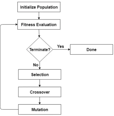
2.1 Common architecture of a genetic algorithm. . . 6

2.2 Example of crossover strategies reproduced from [21] . . . 8

2.3 Example of an utility surface. reproduced from [25] . . . 11

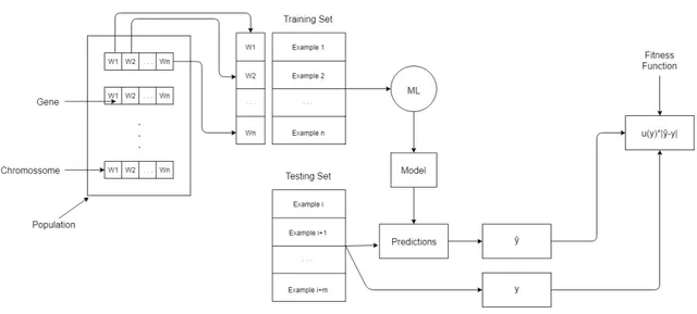
3.1 Architecture of the proposed solution. . . 14

3.2 Example of 1-point crossover. . . 15

3.3 Frequency distribution graph of the target’s variable of an artificial data set with a possible relevance function. P1 - Minimum value; P2 - Median; P3 - Maximum value; . . . 19

3.4 Training set for the artificial data set. . . 21

3.5 testing set for the artificial data set. . . 21

3.6 A) Result of linear regression on the original training set. B) Result of linear regression on the training set obtained by our approach. . . 22

3.7 Weight attributed to each example in training set using our approach. . . 23

3.8 Results regarding Test I: A) Resulting model using our approach. B) Distribution of weights obtained in the training set. . . 24

3.9 Results regarding Test II: A) Resulting model using our approach. B) Distribution of weights obtained in the training set. . . 25

3.10 A) Data set that will be used for training. B) Data set that will be used for testing. 26 3.11 Linear regression model using the original created training set. . . 27

3.12 Results regarding Test I: A) Resulting model using our approach. B) Distribution of weights obtained in the training set. . . 28

3.13 Results regarding Test II with 99% of zeroes per individual: A) Resulting model using our approach. B) Distribution of weights obtained in the training set. . . 29

3.14 Results regarding Test II with 95% of zeroes per individual: A) Resulting model using our approach. B) Distribution of weights obtained in the training set. . . 29

3.15 Training set used in experiment III and corresponding linear regression model. . . 31

3.16 Results regarding Test I of experiment III with 90% of zeroes per individual: A) Resulting model using our approach. B) Distribution of weights obtained in the training set. . . 32

3.17 Distribution of weights obtained for the training set in Test II of experiment III. . 34

3.18 Variation if maximum utility per iteration in Test II of experiment III. . . 35

3.19 Distribution of weights obtained for the training set in Test I of experiment IV. . . 38

3.20 Sequence of distribution of weights obtained for the training set in Test II of ex-periment IV separated by 1000 iterations. . . 39

4.1 Comparison of predictions’ errors between the model with the original training set and Approach I. . . 45

LIST OF FIGURES

4.2 Distribution of weights on the training set. A) Housing training set using sion tree; B) Housing training set using SVM; C) Orders training set using regres-sion tree; D) Orders training set using SVM; . . . 45

4.3 Representation of the utility function used for INOVRETAIL case study. . . 52

4.4 Comparison between real net sales and predicted net sales of Store 7 using real values for conversion ration and footfall. . . 54

4.5 Comparison between real net sales and predicted net sales of Store 7 using pre-dicted values for conversion ration and footfall. . . 55

4.6 Comparison between real net sales and predicted net sales of Store 1. . . 57

A.1 Results regarding Test II with 90% of zeroes per individual: A) Resulting model using our approach. B) Distribution of weights obtained in the training set. . . 62

A.2 Results regarding Test II with 80% of zeroes per individual: A) Resulting model using our approach. B) Distribution of weights obtained in the training set. . . 62

A.3 Results regarding Test II with 60% of zeroes per individual: A) Resulting model using our approach. B) Distribution of weights obtained in the training set. . . 63

B.1 Results regarding Test I of experiment III with 80% of zeroes per individual: A) Resulting model using our approach. B) Distribution of weights obtained in the training set. . . 66

B.2 Results regarding Test I of experiment III with 60% of zeroes per individual: A) Resulting model using our approach. B) Distribution of weights obtained in the training set. . . 66

List of Tables

3.1 Parameters used in experiment I. . . 21

3.2 Parameters that were used to run both tests. . . 27

3.3 Parameters used to run Test I of experiment III. . . 31

3.4 Parameters used to run Test II of experiment III. . . 33

3.5 Parameters used to run Test I and Test II of experiment IV. . . 37

4.1 Information regarding used data sets. . . 42

4.2 Parameters used for data set Servo. . . 44

4.3 Comparison of utility and RMSE values between the two approaches and the ML algorithm in use. In this case the it is used a decision tree for regression. . . 46

4.4 Comparison of utility and RMSE values between the two approaches and the ML algorithm in use. In this case the it is used SVM. . . 47

4.5 Utility results obtained used the expected weight distribution on SVM and Deci-sion Tree algorithms. . . 48

4.6 Information regarding tables provided by INOVRETAIL. . . 49

4.7 Details about stores used in the experiment. . . 51

4.8 Utility results for each store with different setups. . . 55

Abbreviations

DT Decision Tree GA Genetic algorithm ML Machine Learning RF Random Forest

RMSE Root mean squared error SVM Support Vector Machine UBDM Utility-based data mining

Chapter 1

Introduction

Data-driven decisions are an essential way to achieve competitive advantage [23]. This is the process of making a decision which its basis lies within data analysis. One of the most predominant types of analytics is predictive analysis. It takes into account data previously recorded to make predictions of what might happen in the future. It is used in different areas such as marketing, financial services, communications industry, retail, pharmaceuticals, social networking, among others.

Usually, in real-world situations, the problem at hand may not require the discovery of frequent patterns spread throughout the data domain. Sometimes a more insightful data knowledge can be derived if we focus on specific parts of a data set. This knowledge can be translated into high utility as it is significantly impactful on decision making. Therefore, the business user has reasons to be more interested in a lower error on these specific parts of the data set domain rather than others.

One integral part of predictive analysis is model evaluation. It allows the understanding of how a model fits a set of data so we can compare different models. In order to evaluate models, there are standard measures such as Root Mean Squared Error (RMSE), accuracy, among others. Most of these measures do not take into consideration the different error costs throughout the domain of the target variable. Thus these measures are unfit for cost-sensitive tasks. Usually, Machine Learning (ML) algorithms use these metrics to optimize their predictions. Consequently, these algorithms fall short when the cost is not uniform across the domain of data.

Utility-based data mining is a type of cost-sensitive learning where the costs and benefits of the accuracy/error for each prediction are considered differently. This means that instead of attributing a uniform relevance to each instance in our data, such importance may vary with each instance. This data mining branch has a wide range of applications in areas such as fraud detection, catastrophes prediction, network attacks, rare disease diagnosis, among others [24]. On all these scenarios, there is a clear interest in a subset of its domain. Usually, the accuracy on rare examples is the most interesting from the user’s point of view.

The proponent of this thesis is INOVRETAIL1. This is a company that provides data driven

Introduction

solutions to retailers. One of their services is predicting targets for stores. Targets represent a sales goal that an employee has to achieve during his shift. If the employee can meet the proposed goal, he is rewarded. The global target is the sum of all employees target during a day in a store. The proposed problem by INOVRETAIL, and the one which is addressed in this thesis, is to make predictions for net sales values in stores that take into account a store’s potential to grow their sales. For instance, there are days where it is usual to have some operational complications. If these complications were to be properly addressed and solved, it would be possible to increase net sales. As such, an overprediction in this type of days does not hold the same significance as an underprediction.

1.1

Motivation

We are addressing the proposed problem by INOVRETAIL of net sales prediction. In this task, the error costs of predictions varies throughout data’s domain. So, utility-based data mining should be regarded. However, most of these approaches focus on classification problems [27, 13, 12,

6, 31, 26,4, 3, 10]. On the other hand, considering regression problems, research done on the topic is still on the early stages [1,24]. Therefore, this thesis centers exclusively on utility-based regression.

1.2

Goals and contributions

The main goal of this thesis is to develop a wrapper based approach for utility-based data mining. This approach is algorithm-independent, which means it can be used with any ML algorithm.

Regarding our case study, the goal is to use this approach to address the net sales prediction’s problem. In this task, the cost of underprediction and overprediction varies across the data’s domain.As such, we need to define a function that is able to translate these misclassification costs. So, another goal of this thesis is the development of an utility measure for the retail case study.

1.3

Document Structure

The remainder of this document is structured as follows:

• Chapter2, Background, starts by explaining the concept of genetic algorithms and detailing some strategies used on genetic operators. Finally, it introduces the concept of utility-based data mining for classification and regression problems;

• Chapter3, Approach, starts by detailing the developed approaches and justifies some deci-sions made. Some experiments on artificial data used to understand the behaviour of the proposed method are also discussed;

Introduction

• Chapter 4, Empirical study, starts by detailing the experiments done in UCI data sets and discussed the corresponding results. Then, it presents the approach followed on the case study to predict sales goals. Finally, the corresponding results are discussed.

• Chapter5, Conclusions & Future Work, holds the main conclusions and points out possible future works.

Chapter 2

Background

This chapter presents the two main areas of interest for this project, Genetic Algorithms and Utility-based Data Mining.

2.1

Genetic algorithm

Genetic algorithms were introduced by John Holland in the mid-1960 [16]. Darwin’s theory of evolution inspires these algorithms. They are based on the application of different evolutionary operators such as selection, crossover, and mutation to a population of solutions. These types of algorithms are often used in optimization and search problems. A common architecture of a genetic algorithms is presented in Figure2.1.

Genetic algorithms try to combine exploration and exploitation approaches. Exploration con-sists of searching in a global area of the optimization function with the single goal of finding reasonable solutions that are still unrefined. This mechanism prevents the algorithm from being stuck in a local optima. On the other hand, exploitation entails the refinement of a solution that is assumed to be close to the global optimum. Of course, if exploitation is applied to solutions that are not near the optimal solution, it may be a risk that it can be stuck at a local optimum [20].

2.1.1 Fitness function

In every GA, there is a need to evaluate each chromosome according to the goal of the algorithm. This evaluation is performed by a fitness function. It is a domain-specific and user-defined func-tion. This is an integral part of the algorithm as it allows to distinguish chromosomes that are good solutions from those that aren’t. Naturally, chromosomes that carry food genes have a likelier chance of surviving throughout the iterations of the algorithm. Thus, there will be more and more fittest chromosomes as the number of iterations increase. As such, optimizing a fitness function will bring better solutions for the task, which is the goal.

Background

Figure 2.1: Common architecture of a genetic algorithm.

2.1.2 Chromosome representation

In order to use a GA, the design of the chromosome needs to be specified. A chromosome is a set of genes. These genes carry the information of the solution. They translate an encoding method to a domain solution.

Usually, the representation of chromosomes is domain-specific. One of the most common ways of approaching this problem is using binary encoding. In this type of encoding, each gene corresponds to the value 0 or 1. It is also possible to encode chromosomes using a larger range of numeric values. Another type of encoding is string encoding, in which each gene corresponds to a string code.

2.1.3 Population generation

The population is an essential component of genetic algorithms. Chromosomes, which are also referred to as individuals are what composes a population. The algorithm changes values, with the goal of generating better solutions as the iterations go by.

Regarding its generation, there are two main discussion topics: the size of the population and how this population is created. Regarding the size of the population, some studies suggest a low population size can lead to suboptimal solutions [15,22]. However, having a higher population size is computationally costly, and the algorithm may take more time than what is necessary [19,

18]. There are also some studies suggesting that the population size should be proportional to the complexity of the space search [32].

Background

With regards to how the initial population is created, there are two main techniques: randomly generating genes or using a heuristic approach. Usually, random values are used to generate the population. However, it is also possible to use heuristic functions that may generate chromosomes with good fitness. These heuristic functions are associated with increases in maximum fitness when compared to random generation [28]. However, creating all the individuals of the population with a heuristic function can lead to premature convergence, in which turn leads to suboptimal solutions.

2.1.4 Selection

Selection is the process of choosing chromosomes to go to the next generation and discarding the remaining. This is usually a fitness-based process, in which the fittest individuals have a higher chance of being selected. The fitness function is domain-dependent and represents the translation of the problem.

Selection may include elitism. This is when the best individuals of the population are allocated in the next generation unchanged. As such, they do not undergo the process of mutation nor crossover. Saving these individuals for the next generation avoids the loss of the best solutions [9].

2.1.5 Genetic operators

The two most common genetic operators are crossover and mutation. However, it is not required that both of them should be used in a genetic algorithm.

Crossover is the process of selecting two individuals to recombine their genes in order to create two offspring. Two standard ways to recombine genes is uniform crossover and k-point crossover and are represented in Figure2.2. The latter happens when both parents are separated in the same k genes, and each child will have a genetic segment from one parent, followed by the next segment from another parent. In uniform crossover, each gene has an independent probability of being chosen from the corresponding gene of each of their parents.

Usually, mutation is a genetic operator used to maintain population diversity. It alters 1 or more genes in a chromosome. There are two standard approaches to mutation: intergene and intragene. In intergenic mutation, every gene has an independent chance of being mutated, while in intragenic mutation, the chromosome must first be randomly selected for mutation and only then can a gene of that chromosome be randomly replaced. Usually, low mutation rates can lead to premature convergence because of low genome diversity.

2.2

Utility-Based Data Mining

This section defines utility-based data mining and the research done in this field, including both regression and classification problems.

Background

Figure 2.2: Example of crossover strategies reproduced from [21]

2.2.1 Definition

Conventional methods of measuring error such as MAE, MSE, RMSE are inefficient in real-world scenarios [24]. Measuring accuracy in imbalanced data sets can lead to a wrong perception of how good a model can be. This happens because having lower errors in common regions than rare regions of the data set may not be relevant in real-world problems [5]. Moreover, the cost of errors may differ between classes since the main objective could be to have a model that is good at detecting a type of class or outliers. For these scenarios, we need to use a different kind of error measurements that depends on the importance derived from the primary goal of the model. This kind of problems can be expressed as an utility-based data mining problem. Consider the example of a bank deciding whether or not to grant a loan to a set of clients. The goals of the bank can be to minimize the bank loss on granted loans. A bank loses money on a loan if the client is unable to pay for it. So an approach to solving this problem would be to maximize the accuracy of the class of clients that default a loan. Minimizing the error on this class allows the bank to lose less money with this class of clients in detriment of a higher error on the opposing class. Achieving a good accuracy on the former class can be done by having a higher error cost on that class than on the latter class.

Elkan [11] defines utility as a combination of benefits and costs that are specific to the domain of the application. There are two main methods for these type of problems: resampling the training sample and cost-sensitive ML. The first one corresponds to changing the weights of the examples in the training set before applying the ML algorithm. The latter is based on adapting already existent ML algorithms into being cost-sensitive or developing a new one that can maximize utility. For regression problems, utility is defined as a function of both the error of the prediction and the relevance attributed to the domain of the target variable and of the prediction.

Background

State of the art for this field is divided into regression and classification problems as follows in Section2.2.2and Section2.2.3, respectively.

2.2.2 Classification problems

Regarding classification problems, there is a lot of study in different topics. This research entails relational costs in training set examples [27], quantification tasks [13], using evaluation measures as an utility function [12], imbalanced data sets [6], data collection [31], multi and binary classifi-cation tasks [3,10].

In this Section, we will discuss Metacost in greater detail because it is a wrapper approach for classification problems.

Introduced by Pedro Domingos [8], Metacost is a wrapper algorithm that deals with different costs per class. The Bayes optimal prediction is the basis of this method which goal is to minimize the conditional risk R(i|x), i.e., expected cost. The formula is as follows:

R(i|x) =

_∑

j

P( j|x)C(i, j) (2.1)

where P( j|x) is the probability that given an example x it belongs to class j and cost(i, j) is the cost associated with the miss-classification of an example that belongs to class i predicted to belong to class j. This implies a partition of the example space into j regions, with class j being the least costly prediction in the j region. If the miss-classification of class j becomes more expensive than the miss-classification of other classes, then "parts of the previously non-class i regions shall be re-assigned as region i since it is now the minimum expected cost prediction" [29].

This method is a variant of the bagging method (also called bootstrap aggregating). Bagging is an ensemble algorithm that works as follow: given a training set of size s, it generates x new training sets of size s using replacement by sampling uniformly from the training set. Models are produced using each of the training samples created. The results are computed by averaging all the established models for regression or by voting for classification. The difference with Metacost lies on the fact that the number of examples of each generated training set may be smaller than the training set size [8]. It estimates all the class probabilities taking into account all the models made and relabels each training example with a rated optimal class using equation2.2. Finally, the process repeats itself once again with the relabelled training sets to generate the final model.

classx= argmini

_∑

P( j|x)C(i, j) (2.2) One advantage of this approach is that it is a wrapper method as it can be used with any classification learning ML algorithm without prior knowledge of it. The main disadvantage is the processing time since it has to run the ML algorithm s amount of times. Results demonstrate that this approach has reduced costs when compared to error-based classification and stratification. It was also concluded that it scales well with large data sets [8].

Background

2.2.3 Regression algorithms

Despite extensive research on utility-based classification approaches, there is still a lack of re-search in regression problems. Utility is not often considered for these latter problems, even though its importance as it is common to have asymmetric costs [7].

In order for a problem to be considered to have an imbalanced domain and asymmetric domain relevance, one of the following properties must be verified [2]:

1. L(y, y) = L(x, x) ; U(y, y) = U(x, x): perfect predictions may output a different utility value; 2. L(y1, y2) = L(x1, x2) ; U(y1, y2) = U (x1, x2): the same error may output a different utility

value;

3. A combination of the above options.

Ribeiro adressed the problem of utility based regression based on the concepts of relevance functions and utility surfaces [24].

2.2.3.1 Relevance functions

A relevance function is used in attributing importance to values in the data domain according to the application domain. A function φ () maps the target variable’s values to the range [0, 1] where 0 corresponds to the minimum importance and 1 to the maximum relevance.

Branco et al. describes the benefits of this method as follows [2]:

• It is easier to define a relevance function based on the target variable’s domain (y) rather than taking into account two variables ˆyand y;

• Utility functions require more information to be defined when compared to relevance func-tions. The former needs a deeper domain knowledge to be specified.

2.2.3.2 Utility surface

Utility surface is a function that takes into account the relevance of the predicted values and the real ones as well as the error of the prediction and turns it into utility. In [24], utility is a measure of the error between the estimated and actual results as well as the relevance that the domain user attributes to ˆyand y. Figure2.3illustrates an example of a utility surface.

This utility surface is what distinguishes a standard regression problem from an utility-based one. The former assumes the error (L(y, ˆy)) is uniform across the data domain. On the other hand, the latter, besides depending on the same loss function, also takes into account the relevance of the variables ˆyand y.

Background

Figure 2.3: Example of an utility surface. reproduced from [25]

The conditional density of the target variable is used to estimate the utility of a prediction. This conditional density function can be seen in equation2.3where fX,Y(x, y) represents the join

density function of X and Y , and f X (x) is the marginal density of X [1].

f_Y|X(y|X = x) = fX,Y(x, y) fX(x)

(2.3) It was also introduced in [24] a utility measure that best suits utility-based regression problems as demonstrated. The formula is called mean utility and goes as follows:

MU =1 n n

∑

where n is the number of predictions generated, φ the relevance function, p the penalizing costs factor, ˆyrepresents the predicted value and y the real observed value.

2.2.3.3 ubaRules

Proposed by Rita Ribeiro [24], ubaRules is an ensemble method applied to regression problems to optimize a utility function. Its main goal is to obtain an accurate model according to a specified utility measure. The author’s intent was that it should be interpretable for the domain user because relevant values are usually associated with costly/beneficial decisions [24]. Thus the choice of opting for a rule-based formalism for the representation of the models as they are easily under-standable. This ensemble method is divided into the following two steps.

Background

Firstly, different regression trees are generated using various samples from the training set. Regression rules are extracted from these models. A regression rule is defined as follows [24]:

rk(x) = Uk ρ

∏

j=1

I(xj∈ χkj) (2.5)

In equation2.5, χk_j represents a subset of the domain values for input variable j, xjis the value

of x on input variable j, I represents a function which returns 1 or 0 depending on if the argument inside it, is true or false, respectively. ρ is the number of input variables and Uk represents the

constant prediction of rule k for the target variable Y . The rule is equal to Uk if every input

variable satisfy the conjunction of tests proposed by the rule. Otherwise it is equal to 0.

Given that the rules have been obtained from different regression trees, the next step is to choose the rules with which to generate the final model. However the number of rules increases with the number of models used, and although it can improve the accuracy of the model, it may also reduce its interpretability as the complexity of the model increases with the number of rules. So there is a need for a process that reduces the number of rules by selecting only the best ones. Each rule is evaluated individually using a utility metric U . The rules are ordered in decreasing order of their estimated utility to form a ranking system. Finally, the best n rules are selected to generate the final ensemble.

2.2.3.4 Sampling approaches

Most ML algorithms focus on the most common cases on the data sets but may not cover regions that are of the most importance to the user.

In [30], Torgo et al. propose two approaches that are adapted from existing sampling methods. The first one consists of undersampling common values. The goal of this approach is to have a better ratio between common examples, which have reduced importance, and rare cases where its importance is significant.

The second one is an adaptation of SMOTE sampling. SMOTE is a sampling method used for unbalanced data sets in classification problems. It entails adding synthetic examples to the minority class so it has the same occurrence as the majority class. The authors propose that this method should be adapted to regression by defining regions of interest. This approach should oversample the region of interest, which functions as the minority class, and undersample the uninteresting region, which corresponds to the majority class.

Results show that these approaches are significantly better than using the original training set with the same ML algorithm.

Chapter 3

Approach

This chapter presents the proposed wrapper approach for utility-based data mining. It also details experiments performed on artificial data. Finally, it explains how some changes to the approach came to fruition.

3.1

Algorithm formulation

We are assuming that errors in a prediction are not always strongly correlated with its impact on the utility. As such, our approach consists of reweighting the examples in the training process in a way that more importance is given to examples with a higher impact on utility. We reweight the examples by resampling. The question is how how to define the right weights. We follow a wrapper approach, where the method iteratively searches for the best weights, evaluating solutions by learning and testing the model with the proposed weights. The search algorithm is a genetic algorithm.

A chromosome represents the weights assigned to each example (in the training data) and the fitness function is the utility of the model obtained with the training set reweighted according to the chromosome. Thus we could use a genetic algorithm for our resampling strategy.

3.1.1 Chromosome representation

To use genetic algorithms, we need to define what is the population, chromosomes, and genes in our problem (Section2.1). Per the general definition, the population is a set of chromosomes (individuals). In our problem, a chromosome is used to transform the original training set in another that will be used for modelling. The chromosome has a fixed number of genes that is equal to the number of rows in the training set. Genes compose a chromosome and represent the weight of each instance in the training set. So each chromosome functions as a mask of the training set. For instance, if the first gene has the number 10 in it, the first instance of the original training set appears ten times in the new training set. In summary, each gene represents an example from the training set and its value (weight) corresponds to the number of times this example is going to be replicated in this set. Thus we would have the number of times each instance appears in the

Approach

Figure 3.1: Architecture of the proposed solution.

training set changing throughout the algorithm. The goal is to find the best combinations of genes that optimize a fitness function.

3.1.1.1 Fitness function

When we test the fitness of each chromosome, we use a fitness function. In this case, our fitness function is the utility evaluation metric. Firstly, to evaluate each individual of the population, we need to use the new generated training set to create a model. Then we measure the performance of this model on a testing set using a utility metric (3.1). The utility of a chromosome is given by equation3.1, where i is an instance from the testing set, n the total number of cases in this set, yi

the real value of the target variable, ˆyi the prediction value, and u(y) the importance attributed to

this instance of a testing set. This formula represents the preference of the error in the domain of the target variable. Since this formula is proportional to the error on the predictions, we want to minimize its output. However, GA tries to maximize their fitness functions. To handle this issue, we used equation3.2to transform the minimization problem into a maximization one. At the end of the selection process, we have the same number of individuals that we had at the beginning.

U(c) =

n

∑

i

u(y) ∗ |(yi− ˆyi)| (3.1)

U S= 1

U(c) + 1 (3.2)

The following sections describe the GA operations such as selection, crossover, and mutation. We developed two approaches based on the same concept. The second was developed based on preliminary experiments with the first one but, for convenience, we describe both of them before the experiments. As such, for clarity purposes, the first approach is referred to as Approach I, while the latter approach is referred to as Approach II. These approaches differ in the selection

Approach

Figure 3.2: Example of 1-point crossover.

and mutation stages. Therefore, in the next sections, these operations are going to be divided into subsections for each of the strategies.

3.1.2 Selection process

This section details the selection process used for Approach and Approach II.

For Approach I, at the beginning of each iteration of the algorithm, the population must be evaluated according to a fitness function in order to use roulette wheel. The fittest individuals according to this function have a higher chance of being selected for the next phase. However, in our algorithm, we also guarantee the n fittest individuals are present in the crossover step. This process differs from the general elitist approaches as the chosen individuals go through crossover and mutation, unlike standard elitist methods. We chose this strategy as modeling of an individual is a costly process, and disregarding some individuals for crossover and mutation seemed wasteful. As for Approach II, after evaluating the fitness of each individual of a population, these are ordered by their fitness value. The worst n individuals are removed from the population. The best nindividuals are replicated once, creating two sets of these individuals. The first set goes directly into the next iteration without going through crossover or mutation processes. The second sample joins the rest of the population in crossover and mutation.

3.1.3 Crossover operator

In the crossover, we generate chromosomes by combining two of the parents of the population. Parents are randomly selected for the process. Some individuals may not participate in this task as they may not be selected. This operator is associated with a probability. Since each chromosome has an independent probability of being selected, that may not happen for all cases. There are many crossover strategies, but we chose to implement single point crossover (3.2). The reason behind this choice was the building block hypothesis [14]. This hypothesis consists of recombining building blocks, which are low order sequences of genes with above average fitness. In our case, the examples of the training set are ordered according to their target variable. As such, a building block could be a part of the domain which is given a high or low relevance.

Approach

3.1.4 Mutation operator

Mutation consists of replacing gene values by other values which are randomly generated. There are two types of mutation operators, intragene and intergene. Intragene mutation requires that an individual is randomly drawn for mutation and then one or more genes from that individual are changed to other randomly generated values. In intergenic mutation each gene has an independent probability of being mutated. In our algorithm, we opted for the intergenic mutation the mutations have a higher chance of being more equally dispersed between the chromosomes. Thus, we have a higher probability of changing more chromosomes per iteration.

3.1.4.1 Mutation process I

This process in Approach I is a common intergenic mutation with a fixed rate. Each gene has an independent probability of being changed to another value randomly generated.

3.1.4.2 Mutation process II

In this strategy, the mutation is not a fixed value but rather a varying one. At the beginning of the algorithm, the mutation rate is set to a high value. Then we must define a parameter i which represents the number of iterations needed for the mutation rate to drop while the best solution found remains unchanged. For instance, if i is equal to 10, it would require ten iterations for the mutation rate to drop. However, if the utility of the fittest individual increased, the counter is reset. In this situation, it would take another ten iterations for the mutation rate to decrease. The mutations rate is reduced by a determined factor r. It stops dropping when it hits the minimum mutation rate specified. Algorithm1translates the specified operator into pseudo-code.

3.2

Utility measures

Utility functions quantify the importance of different areas of the data domain. The utility func-tion is typically determined by the applicafunc-tion domain. However, to validate the approach we would like to test it on artificial data and also benchmark data sets. This is also important for reproducibility, as the data from the case study used in this project is not public domain. Thus, we need to arbitrate a utility function for the experiments with artificial and benchmark data. As in some real-world problems, there is a more significant interest in extreme and rarer values on the data domain [24], we followed the same line of thought. As such, we give more importance to values that are on the extreme of the data domain rather than the middle of it. In our methodology, we are relaxing the definition of a utility function to a relevance function in order to simplify our experiments.

We test this approach on data sets which target variable has more examples in the middle of its domain rather than the extremes. For instance, if the domain of the target variable resembles a normal distribution, it is guaranteed that we have more examples in the middle region and fewer instances in the extremes. Thus it allows us to accomplish our goal of attributing higher importance

Approach

Algorithm 1: Mutation for Approach II. mut_i ←− initialmutationmutationvalue; mut_ f ←− lowestmutationvalue;

dec_r ←− decayingrateo f themutation;

n←− numbero f iterationswithoutimprovementstodecreasethemutationrate; begin counter←− 0; best_solution ←− 0; current_mutation ←− mut_i; while genetic_algorithm_termination_condition do if current_solution > best_solution then

best_solution = current_solution; counter= 0; else counter+= 1; end if counter == n then

current_mutation = current_mutation x dec_r; counter= 0;

end

if current_mutation >= mut_ f then current_mutation = mut_ f ; end

end end

Approach

to extreme values rather than values located in the middle of the data domain. If this does not occur, it will not bear meaning to use this utility measure to demonstrate how our algorithm works as the values on the extremes would be common and easily predicted. Moreover, the utility function should adapt to the scale of the target variable. As such, it is data-independent, i.e., can be used with any data sets without previous knowledge.

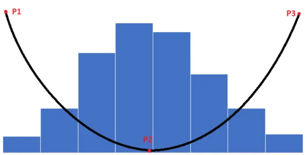
Figure3.3represent how the variable Y is distributed across the domain for an artificial data set. As previously said, it is essential that these data sets’ distribution is similar to a normal distribution to create our utility measures. As we can see from that figure, the closer the examples of Y variable gets to the extremes, the less frequent they are. This allows us to create a utility metric by giving more importance to extreme cases and lesser significance to examples around the mean. Taking into account the distribution in figure3.3, we can calculate the displayed utility function in three steps. Firstly, we find the minimum (P1), maximum (P3) and median (P2) value of the target variables (Y ). Then we calculate a positive quadratic function, which we will call F1, using P2 as the minimum and P1 as an auxiliary point. Lastly, we calculate a quadratic function F2 with the values P2 and P3 following the same logic. We end up with two equations F1 and F2. When evaluating a model on a testing set, if the value of the target variable is lower than the median, we use F1, while if its higher we use F2.

The reasoning behind this decision of having two quadratic functions was to correct the possi-bility of our target variable being skewed towards one of the sides. If the right side of the median, which corresponds to the side which the maximum is in, represented considerably higher impor-tance than the left side it would devalue the imporimpor-tance given to the left side and thus would not meet the purpose of the experiments. For instance, in the previously mentioned data set, if the maximum of the Y variable is 1, and we would only use one quadratic equation, it would result in a significant discrepancy between the two extremes of the data domain.

As we can notice, figure3.3 does not have a vertical axis. Its absence happens because we want to be able to set y-coordinate of the aforementioned points to whatever we see fit. With that in mind, we established that P2 would still be given a positive value as its y-coordinate because we want it to carry importance higher than 0, however small that influence may be. Regarding the values of P1 and P3, we used different values as its y-coordinate. By attributing different values, we could be able to change the curve and analyze how it behaves with our approach. This parameter will be referred to as K. Equation3.3details the formulation of the utility function with b being the minimum importance given to the the median, k the maximum importance given to both extremes, and m the values of the maximum and the minimum of the domain depending on what quadratic function is being formulated.

Approach

Figure 3.3: Frequency distribution graph of the target’s variable of an artificial data set with a possible relevance function. P1 - Minimum value; P2 - Median; P3 - Maximum value;

3.3

Experiments

In this section, we will discuss some experiments done with artificial data and the obtained results. These experiments were made so that we can validate our approach. We are also analyzing the best training set obtained, i.e., the weights attributed to the examples in the training set.

3.3.1 Experiment I

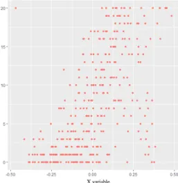
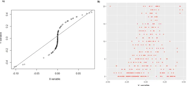
Firstly we are going to test the approach using the artificial data set. Let us consider the construc-tion of the following data set. Firstly, we randomly create a list of 1000 numbers that range from -0.5 and 0.5 of mean 0 and standard deviation of 0.2. We will refer to this list as Y . Then we create the X variable that results from cubing all the numbers in Y . The final data set consists of aggregating the variablesX and Y , where Y is the target variable. Thus Y should have fewer examples on the extremes and more in the middle. This data set is randomly divided into a testing set and training set. 75% of the examples are placed in the training set, and the remaining 25% is placed in the testing set. Figures3.4and3.5represent the obtained training set and testing set respectively.

Lorem ipsum dolor sit amet, consectetuer adipiscing elit. Ut purus elit, vestibulum ut, placerat ac, adipiscing vitae, felis. Curabitur dictum gravida mauris. Nam arcu libero, nonummy eget, consectetuer id, vulputate a, magna. Donec vehicula augue eu neque. Pellentesque habitant morbi tristique senectus et netus et malesuada fames ac turpis egestas. Mauris ut leo. Cras viverra metus rhoncus sem. Nulla et lectus vestibulum urna fringilla ultrices. Phasellus eu tellus sit amet tortor

Approach

gravida placerat. Integer sapien est, iaculis in, pretium quis, viverra ac, nunc. Praesent eget sem vel leo ultrices bibendum. Aenean faucibus. Morbi dolor nulla, malesuada eu, pulvinar at, mollis ac, nulla. Curabitur auctor semper nulla. Donec varius orci eget risus. Duis nibh mi, congue eu, accumsan eleifend, sagittis quis, diam. Duis eget orci sit amet orci dignissim rutrum.

Nam dui ligula, fringilla a, euismod sodales, sollicitudin vel, wisi. Morbi auctor lorem non justo. Nam lacus libero, pretium at, lobortis vitae, ultricies et, tellus. Donec aliquet, tortor sed accumsan bibendum, erat ligula aliquet magna, vitae ornare odio metus a mi. Morbi ac orci et nisl hendrerit mollis. Suspendisse ut massa. Cras nec ante. Pellentesque a nulla. Cum sociis natoque penatibus et magnis dis parturient montes, nascetur ridiculus mus. Aliquam tincidunt urna. Nulla ullamcorper vestibulum turpis. Pellentesque cursus luctus mauris.

Nulla malesuada porttitor diam. Donec felis erat, congue non, volutpat at, tincidunt tristique, libero. Vivamus viverra fermentum felis. Donec nonummy pellentesque ante. Phasellus adipiscing semper elit. Proin fermentum massa ac quam. Sed diam turpis, molestie vitae, placerat a, molestie nec, leo. Maecenas lacinia. Nam ipsum ligula, eleifend at, accumsan nec, suscipit a, ipsum. Morbi blandit ligula feugiat magna. Nunc eleifend consequat lorem. Sed lacinia nulla vitae enim. Pellentesque tincidunt purus vel magna. Integer non enim. Praesent euismod nunc eu purus. Donec bibendum quam in tellus. Nullam cursus pulvinar lectus. Donec et mi. Nam vulputate metus eu enim. Vestibulum pellentesque felis eu massa.

Quisque ullamcorper placerat ipsum. Cras nibh. Morbi vel justo vitae lacus tincidunt ultrices. Lorem ipsum dolor sit amet, consectetuer adipiscing elit. In hac habitasse platea dictumst. Integer tempus convallis augue. Etiam facilisis. Nunc elementum fermentum wisi. Aenean placerat. Ut imperdiet, enim sed gravida sollicitudin, felis odio placerat quam, ac pulvinar elit purus eget enim. Nunc vitae tortor. Proin tempus nibh sit amet nisl. Vivamus quis tortor vitae risus porta vehicula.

Fusce mauris. Vestibulum luctus nibh at lectus. Sed bibendum, nulla a faucibus semper, leo velit ultricies tellus, ac venenatis arcu wisi vel nisl. Vestibulum diam. Aliquam pellentesque, augue quis sagittis posuere, turpis lacus congue quam, in hendrerit risus eros eget felis. Maecenas eget erat in sapien mattis porttitor. Vestibulum porttitor. Nulla facilisi. Sed a turpis eu lacus commodo facilisis. Morbi fringilla, wisi in dignissim interdum, justo lectus sagittis dui, et vehicula libero dui cursus dui. Mauris tempor ligula sed lacus. Duis cursus enim ut augue. Cras ac magna. Cras nulla. Nulla egestas. Curabitur a leo. Quisque egestas wisi eget nunc. Nam feugiat lacus vel est. Curabitur consectetuer.

Suspendisse vel felis. Ut lorem lorem, interdum eu, tincidunt sit amet, laoreet vitae, arcu. Aenean faucibus pede eu ante. Praesent enim elit, rutrum at, molestie non, nonummy vel, nisl. Ut lectus eros, malesuada sit amet, fermentum eu, sodales cursus, magna. Donec eu purus. Quisque vehicula, urna sed ultricies auctor, pede lorem egestas dui, et convallis elit erat sed nulla. Donec luctus. Curabitur et nunc. Aliquam dolor odio, commodo pretium, ultricies non, pharetra in, velit. Integer arcu est, nonummy in, fermentum faucibus, egestas vel, odio.

Sed commodo posuere pede. Mauris ut est. Ut quis purus. Sed ac odio. Sed vehicula hendrerit sem. Duis non odio. Morbi ut dui. Sed accumsan risus eget odio. In hac habitasse platea dictumst. Pellentesque non elit. Fusce sed justo eu urna porta tincidunt. Mauris felis odio, sollicitudin sed,

Approach

Figure 3.4: Training set for the artificial data set.

Figure 3.5: testing set for the artificial data set.

volutpat a, ornare ac, erat. Morbi quis dolor. Donec pellentesque, erat ac sagittis semper, nunc dui lobortis purus, quis congue purus metus ultricies tellus. Proin et quam. Class aptent taciti sociosqu ad litora torquent per conubia nostra, per inceptos hymenaeos. Praesent sapien turpis, fermentum vel, eleifend faucibus, vehicula eu, lacus.

Nulla malesuada porttitor diam. Donec felis erat, congue non, volutpat at, tincidunt tristique, libero. Vivamus viverra fermentum felis. Donec nonummy pellentesque ante. Phasellus adipiscing semper elit. Proin fermentum massa ac quam. Sed diam turpis, molestie vitae, placerat a, molestie nec, leo. Maecenas lacinia. Nam ipsum ligula, eleifend at, accumsan nec, suscipit a, ipsum. Morbi blandit ligula feugiat magna. Nunc eleifend consequat lorem. Sed lacinia nulla vitae enim. Pellentesque tincidunt purus vel magna. Integer non enim. Praesent euismod nunc eu purus. Donec bibendum quam in tellus. Nullam cursus pulvinar lectus. Donec et mi. Nam vulputate metus eu enim. Vestibulum pellentesque felis eu massa.

For this experiment, the parameters used are detailed in Table3.1. The initial population is generated randomly from values of 5 to 20, with a mean of 10 and a standard deviation of 3. All elements of the population are available for crossover and mutation. The ML algorithm used was linear regression. Regarding the utility metric, we used the one explained in Section3.2 with a simple modification: all examples in the training set which Y variable is between -0.25 and 0.25 do not contribute to the utility value, i.e., their error is not considered for utility purposes.

Parameters for tests run Parameter Test Training set size 5

Population size 10 Elitist rate 10% Crossover rate 75% Mutation rate 0.2% Number of iterations 10000 K 20

Approach

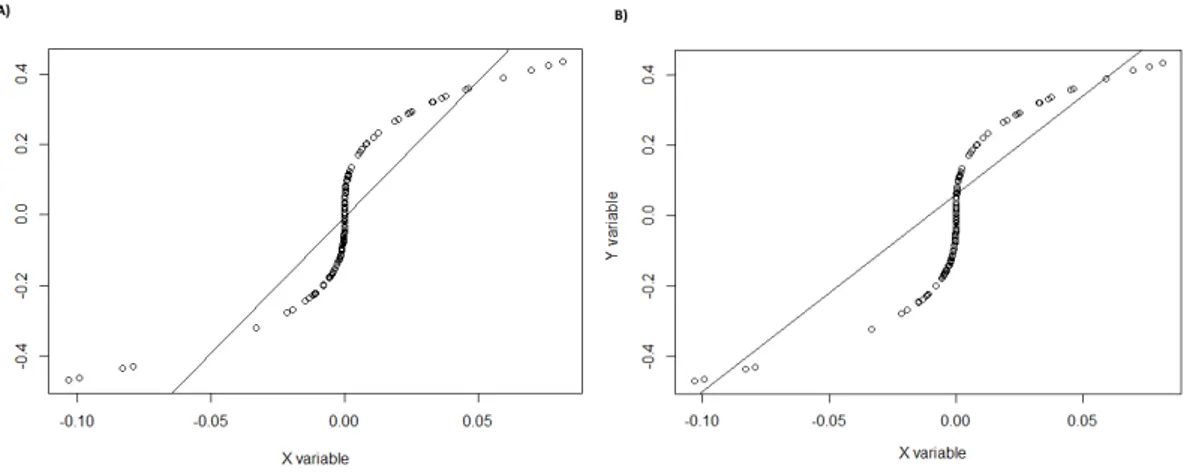
Figure 3.6: A) Result of linear regression on the original training set. B) Result of linear regression on the training set obtained by our approach.

Figure3.6compares our approach I with a linear regression algorithm and the linear regression model with the original training set. As it was expected using our method, we got a model that better fits our utility function. This fitness can be verified by comparing the angle between the line and X axis wherein our approach the angle is smaller. Consequently, the line is closer to the extremes of the target variable (Y ), which we attribute higher importance. Moreover, the value of utility using our approach is 0.049 while using the original data set is 0.026. Even though there is a small difference between utility values, when looking at the produced models, we can see a clear difference.

Figure3.7 shows the best distribution of weights per training set example we were able to achieve. We expected that the weights would reflect our utility measure. So if an example was in an area of great importance, its weight should be higher. However, this does not necessarily happen (Figure 3.7). We found out that it indeed gives higher weights to the extreme examples, though in the left side of this figure we only have one instance with maximum weight and right next to it there is a significant drop. This fall can be explained by looking at our training set and testing set distribution in Figures3.4 and3.5. We can see that the training set has only 1 example near the highest value region while the next one is still at a relatively large distance from the former. We believe that if the algorithm had given higher importance to the second lowest example in the training set, according to Y variable, it would lower the utility value formerly obtained. This assumption was proven correct by manually changing the obtained distribution. Looking at the right side of the figure, we can see that there are a lot more examples that are near the maximum weight. Comparing with the left side, there are more examples in higher importance areas on the right side, where the Y value is higher than on the left. This could be used to justify the higher weights on that region. We can also verify that there is a drop in weights just like it happened on the left side of the figure. The most exciting aspect and the one we were not expecting is the region in the middle. There are a lot of examples that have a high weight associated with them

Approach

Figure 3.7: Weight attributed to each example in training set using our approach.

even though they are in the area that doesn’t contribute to the utility function. This region is a little skewed to the right because there are more values on the right side than on the left in the training set. Our hypothesis for this result is that examples that are next to regions of really high relevance affect more the resulting model than examples on the middle part where the Y variable is close to 0. So the weights attributed to the middle would work as a sort of balancing mechanism to the linear regression model.

We decided to run a few more tests to see if this behavior was consistent. The tests are as follows:

• Test I - We used the same approach as before with the same training and testing sets. How-ever in this case when calculating utility we would only look at two values from the testing set - the minimum and the maximum. The genetic operators used are the same as the first test. It would be expected that the regression model would come closer to both extreme points.

• Test II - We combined the former training and testing set as our new training set and created a new testing set. This sample is composed of 100 values which the Y variable ranges from -0.5 to 0.5 equally separated by 0.01 and the X variable is the cubing of the Y values. The genetic operators and utility function used are the same as the first test. As the test set is symmetric, it should be more noticeable the appearance of a pattern on the weight distribution.

The resulting model and distribution of weight for Test I are represented in Figure 3.8. We can observe that the line is close to the points that represent the maximum and the minimum of the Y variable. Thus it is working as would be expected. However, it is unlikely that this is the best model possible to be achieved. When looking at the obtained distribution of weights, we can see a clearer image of what was captured before. It is attributed a higher importance to both of

Approach

Figure 3.8: Results regarding Test I: A) Resulting model using our approach. B) Distribution of weights obtained in the training set.

the extreme regions, right and left. Then appears a fall in relevance attributed to the next closest examples. After that, it starts increasing again as it gets nearer to the middle.

The resulting model and distribution of weight for Test II are represented in Figure3.9. When analyzing the obtained model, we can see that the line is inclined towards the region of most significant importance.

Concluding this experiment, we can verify that Approach I behaves similarly throughout the different tests. So we hypothesize that the fall that happens in the distribution is due to those areas being the ones that most negatively affect utility. On the other hand, the ones in the middle does not hurt as much because they are near the region the line should cross. They can also work as a balancing mechanism that applies small changes to the linear model without affecting it significantly. Consequently, it makes sense that the algorithm is not prioritizing these changes and instead is focusing on the regions where the dip in weights happens.

Regarding the obtained models, we can notice the approach is working towards a good so-lution, but there is not clear evidence of how good the obtained model is when compared to the optimal solution. This uncertainty is due to the range of possible combinations available. Using a training set of 375 examples in which the weights may vary between 0 and 20 gives 21375possible combination of possible training samples. Since this number is too high, it is computationally unfeasible to test all the possible models. However, it is our opinion that the algorithm is not be-ing given enough time to compute to achieve a better solution. This inefficiency mainly happens because there are too many values that may need to change.

Approach

Figure 3.9: Results regarding Test II: A) Resulting model using our approach. B) Distribution of weights obtained in the training set.

3.3.2 Experiment II

In the second experiment, we addressed some of the limitations of the previous one (section3.3.1), namely regarding the difficulties in evaluation and the complexity of the search space.

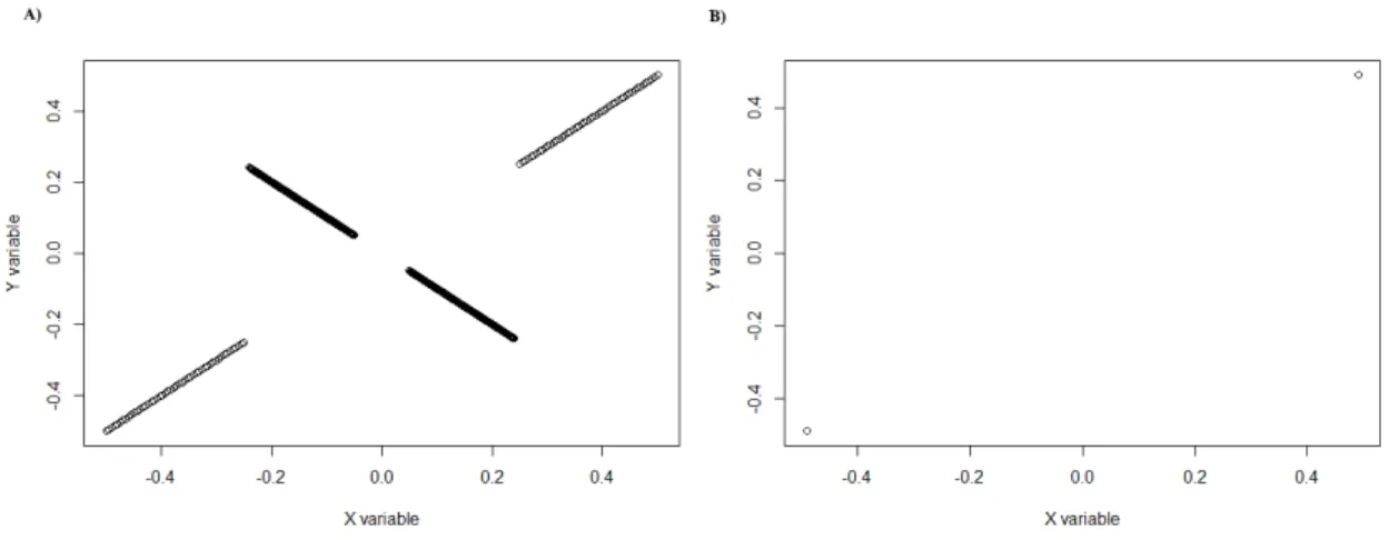
Regarding the difficulty in evaluating of the model and how close it is to the best possible solution, we decided to create a new data set in which we would be able to know which is the perfect model. The data set is organized as follows: for the Y variable, we have four aggregated sequences. The first one is composed of 450 values that range from 0.05 to 0.24 equally dis-tanced between themselves by 0.000423. The second sequence is constituted by 450 values that range from -0.05 to -0.24 equally distanced between themselves by 0.000423. For both of these sequences, the X variable corresponds to −Y . The third sequence consists of 50 values that range from 0.25 to 0.5 equally distanced between themselves by 0.0051. Finally, the last series com-prises 50 values that range from -0.25 to -0.5 equally distanced between themselves by 0.0051. For both of these sequences, the X variable is equal to the Y variable. This data set will be used for training of the linear regression model. Regarding the testing sample, it is composed of only two examples. These examples are the points which the coordinates are (-0.49,-0.49) and (0.49,0.49). A representation of the training and test sets can be observed in Figure 3.10. When looking at the training set, we can see that the vast majority of examples (90%) forms a line with a negative slope. Thus these examples will have significant impact in a linear regression model. This impact can be verified by looking at the resulting model using this training set in Figure3.11. However, when looking at our testing set, we can notice that the generated model has a very bad utility value because the line does not come close to any point on this set. From the perspective of the utility function defined, we expect that the weights in the middle would gradually decrease to 0 while

Approach

Figure 3.10: A) Data set that will be used for training. B) Data set that will be used for testing.

the weights in the extremes would increase significantly. Using this training set to learn a model that maximizes utility, the weights of examples with Y ∈ [−0.24, 0.24] should be very low or even zero.

Concerning the search space, we carried out two tests. The first one (Test I) is a small scale of the training set mentioned earlier, containing only five examples where there are three in the middle region and one in each extreme. This test should be simple enough that the algorithm should find the best model within a few iterations. The second test (Test II) consists of changing a percentage of the initial population weights to zero. The population is randomly generated as detailed in Section3.3.1. However, after we have obtained the initial set of individuals, we change a fixed percentage of values to zero. This is done in a way that guarantees that the set of weights for each example in the initial population include a zero and a non-zero value. In other words, for each training example, there will be at least one chromosome which has a zero value in the corresponding gene and at least one other chromosome with a non-zero value in the corresponding gene. What we are expecting is that by setting a large number of weights to zero it would decrease the computational effort of the algorithm to find the best solution. The parameters for both tests in this experiment are defined in Table3.2.

After running Test I, we were able to obtain the results shown in Figure3.12. As expected, we obtained the perfect fit for our data. The values in the middle region were all given weights of zero, while the two values on the extremes were given non-zero values. As a consequence, the resulting linear model crosses the two points. Thus the model is achieving the maximum utility. Since this test only had five examples in the training set, it only serves as a proof of concept.

For Test II we ran the algorithm with different percentages of zeroes per individual: 99%, 95%, 90%, 80%, 60% as is specified in Table3.2. What we were expecting is that as we decrease the percentage of zeroes, it would become harder and would take longer for the algorithm to find the best distribution. Figures3.13,3.14,A.1,A.2andA.3represent the results obtained from this Test II. With a 99% of zeroes per individual, we can obtain a very good model as Figure3.13shows.

Approach

Figure 3.11: Linear regression model using the original created training set.

Parameters for tests run

Parameter Test I Test II Training set size 5 1000

Population size 10 100 Elitist rate 10% 10% Crossover rate 75% 75% Mutation rate 0.2% 0.2% Number of iterations 10000 10000 K 20 20

Percentage of zeroes non-applicable 99%,95%,90%,80%,60% Table 3.2: Parameters that were used to run both tests.

Approach

Figure 3.12: Results regarding Test I: A) Resulting model using our approach. B) Distribution of weights obtained in the training set.

At first sight, it resembles a perfect model because the line appears to cross those two points in the testing set. But there still exists an error however small it may be. Thus this model is not perfect. This inference is corroborated by looking at the distribution of weights and notice that there are two examples in the middle that are given non-zero weights. Thus the utility obtained is close to the maximum value but has yet to reach the optimal solution.

Interestingly enough, when we try to modify the weight of each of those examples individually to zero, we obtain a lower value of utility. This occurrence means that the only way that we can achieve the perfect model is to change both of those weight to zero at the same iteration. This training set has 1000 examples in it, and with a mutation rate of 0.2%, we can expect an average of two mutations per individual and iteration. Moreover, these two mutations should occur to the individual that has this distribution. Also, the two examples of the training set must be those specific two examples that have a non-zero value. Furthermore, the mutations that can range in the interval [0; 20] must randomly select the value zero for both of those examples. We can see that although it is not impossible to achieve the best model, it seems rather unlikely that we would reach it in a reasonable time.

When comparing Figure3.13with Figure3.14, we can see that the obtained linear regression model is pretty identical. Nonetheless, the latter is slightly worse, with more errors that generate a lower utility value. Furthermore, there are more examples in the middle region that are non-zero, which justifies the lower utility. One thing to notice is that almost all those non-zero weight values are near the very middle of the graph. The closer the Y variable is to 0.05 and -0.05 which are the absolute minimums possible obtainable from our training set, the less impact they have on the model. So the algorithm is "cleaning" the examples that are on the outer sides of the middle region first because they have more of a negative impact on the model.

Approach

Figure 3.13: Results regarding Test II with 99% of zeroes per individual: A) Resulting model using our approach. B) Distribution of weights obtained in the training set.

Figure 3.14: Results regarding Test II with 95% of zeroes per individual: A) Resulting model using our approach. B) Distribution of weights obtained in the training set.