M
ESTRADO
M
ATHEMATICAL
F
INANCE
T
RABALHO
F
INAL DE
M
ESTRADO
D
ISSERTAÇÃO
C
LASSIFICATION OF
2
X
2
F
ICTITIOUS
P
LAY
M
ARIA
F
ERREIRA
V
ILA
L
UZ
M
ESTRADO EM
M
ATHEMATICAL
F
INANCE
T
RABALHO
F
INAL DE
M
ESTRADO
D
ISSERTAÇÃO
C
LASSIFICATION OF
2
X
2
F
ICTITIOUS
P
LAY
M
ARIA
F
ERREIRA
V
ILA
L
UZ
O
RIENTAÇÃO
:
J
OSÉ
P
EDRO
R
OMANA
G
AIVÃO
Resumo
Teoria de jogos ´e uma teoria no ramo da matem´atica criada com o objectivo de estudar e modelar eventos onde duas ou mais pessoas interagem entre si. O objectivo desta teoria ´e perceber como fazer escolhas ´optimas quando se est´a perante um conflito. Existem v´arios tipos de jogos, no entanto, ao longo deste trabalho final de mestrado, foc´amos o nosso estudo num tipo particular de jogos, os jogos evolucion´arios.
Este ´e um tipo de jogo, onde ao longo do tempo, as estrat´egias de cada jogador se adaptam e convergem, em geral, para um equil´ıbrio. Desta forma, os jogadores n˜ao precisam de agir racionalmente. Um caso especial dos jogos evolucion´arios s˜ao os jogos fict´ıcios entre dois jogadores, cada um com duas estrat´egias.
O nosso objetivo foi precisamente demonstrar que ao longo do tempo ex-iste a convergˆencia do processo adaptativo para um equil´ıbrio. Para melhor compreender este processo de convergˆencia, cri´amos uma fam´ılia de exem-plos onde sintetiz´amos todos os jogos fict´ıcios entre duas pessoas com duas estrat´egias cada.
Palavras-chave: Teoria de jogos, Jogos Fict´ıcios, Dinˆamicas da melhor resposta, Equil´ıbrio de Nash, Classifica¸c˜ao
Abstract
Game Theory is a mathematical theory that emerged with the aim of study-ing and modellstudy-ing events between two people. The goal of this theory is to understand how to make the best choice of strategy when we are facing a conflict. There are many types of games but throughout this dissertation we focused in evolutionary games. These are games that are repeatedly infinitely. Over time there is a dynamic adaptation of the strategies, the equilibrium comes naturally and therefore, the players do not use their ra-tionality. Within this type of games there are a particular game between two people which is known as fictitious play. We focused our study in these type of games when both of the players have two strategies. Our goal was to show that, over time, the system will converge to the equilibrium. In or-der to better unor-derstand this interaction we developed a family of examples where we synthesized all the possible combinatorially types.
Keywords: Game theory, Fictitious play, Best response dynamics, Nash equilibrium, Classification
Acknowledgments
O meu principal e maior agradecimento ´e para o meu orientador Professor Doutor Jos´e Pedro Gaiv˜ao, pela sua enorme disponibilidade, por todo o apoio e empenho absoluto. Pelos muitos conhecimentos que me foi trans-mitindo ao longo de todo este trabalho, pelas opini˜oes e pelas cr´ıticas.
Agrade¸co tamb´em a toda a minha fam´ılia e amigos que me foram apoiando e incentivando ao longo de toda a minha etapa acad´emica. Agrade¸co espe-cialmente aos meus Pais por serem um grande exemplo de trabalho e ded-ica¸c˜ao.
Por ´ultimo mas n˜ao menos importante, queria agradecer `a Professora Ana Margarida Neto pelo enorme apoio que me deu ao longo de todo o meu percurso no ISEG, pela disponibilidade, ajuda e bons conselhos que me foi sempre dando.
Contents
1 Introduction 5
2 Basics concepts in Game Theory 8
2.1 Two Player Games . . . 9
2.1.1 Nash Equilibrium . . . 10
3 Fictitious Play Dynamics 19 3.1 Discrete-time fictitious play . . . 20
3.2 Continuous-time fictitious play . . . 22
3.3 Uniqueness of fictitious play flow . . . 24
4 Analysis of 2⇥ 2 Fictitious Play 26 4.1 Indi↵erence sets . . . 26
4.1.1 Identification of the indi↵erence sets . . . 27
4.1.2 Examples . . . 32
4.1.3 Combinatorially distinct types . . . 36 5 Conclusions and Further Research 39
Chapter 1
Introduction
At any moment the economic agents, families and companies have to make decisions. In several interaction situations, the agents are forced to act strategically.
Game theory leads with strategic interactions among multiple (2 or more) decision makers, to which we usually call players. For every game, each one of the players has an objective function associated, which is de-fined according to their own preferences. We assume that the players are rational and so, they are able to order their strategies given their conjec-tures or beliefs on how the other players are going to play. If they get more utility maximizing the objective function, this one is called utility function or a benefit function. On the other hand, if their utility is greater when they minimize the objective function, we can call that cost function or lost function. Usually, the objective function of a player depends on the choices of the other players. Consequently, a player cannot simply optimize his own objective function independently of the choices of the other players.
In other words this means that the decisions made by one of the agents are conditioned by the behaviour or expected behaviour of the opponent. Game theory consists exactly in the study of how the agents react when they are confronted into these interaction situations. In order to maximize his payo↵, each player needs to examine carefully the game conditions. It is required to identify his and the opponent available strategies, to analyse which are the results, associated to each strategy combination, to check the available information to each participant and to know the specific moments when the decisions are made. The game theory can be applied into several fields from economics to biology through social relations. Summing up, any situation where the agents get into a direct relation in order to achieve
certain results.
To define a game we need the number of agents, the number of strategies that each one of the agents has and the payo↵ associated to each strategy combination.
To a more comprehensive introduction to the fundamentals of game the-ory see one of the earliest work that started game thethe-ory in its modern form, Morgenstern & von Neumann. (1944).
There are three types of games: static, sequential and evolutionary games.
Static games are when the participants make their choices simultaneously (see Brown (1951)).
Sequential games, which are dynamic games since strategies are not cho-sen simultaneously but rather sequentially. Here the dynamics is limited to the reaction that a player has at a given moment against the action of another or other agents in the previous time period. In this case there is no dynamic rule able to determine the whole course of the game.
Evolutionary games are e↵ectively dynamic games, (see Hofbauer & Sig-mund (1998)). They rely on a mechanism that allows us to understand how the strategies can evolve over time. In these games there is one more impor-tant element to have into consideration, a dynamic rule that can change pay-o↵ and the behaviour of the players over time. Here we are expecting that, after a transitional period, the game will converge to a dominant long-term equilibrium. In that point, the agents must have adopted an evolutionary stable strategy, meaning, a strategy that they will no longer abandon unless some external force disrupts the game’s underlying conditions.
The major di↵erence between static game and evolutionary game is that the first one admits players as completely rational, able to identify immedi-ately the dominant strategy. Contrariwise, the second one predicts a grad-ual adjustment, in which the set of players will progressively change to the dominant strategy, so that the equilibrium is only reached after the dynamic transition phase has been exhausted.
Throughout this dissertation our main focus will be in this last type of games. If the game theory is defined as the science that studies the strategic behaviour, the theory of evolutionary games is the science that studies the robustness of strategic behaviour. In evolutionary games there is an implicit acknowledgement that the agents learn and evolve over time. The strategy that they choose from beginning of the game can be di↵erent the strategy that maximizes their payo↵. The systematic interaction with the opponents will take them to modify their behaviour over time. We focused our study in a specific case of evolutionary games, called Fictitious
Play. It was introduced by George W. Brown in 1951 (see Brown (1951)). It consists in two players having a finite number of pure strategies. They play repeatedly in such a way that at each round, they use a myopic pure best response against the empirical strategy distribution of his opponent. Fictitious Play can be in discrete-time or in continuous-time.
Initially, in Chapter 2, we will present some basic concepts and notations about game theory. These will be very useful to better understand the rest of our work. Our focus will be on two player games given by a bimatrix.
Next, in Chapter 3, we introduce the learning dynamics called Fictitious Play and we go deeper into this subject. Here we present and discuss a geometric representation of the strategy space.
Chapter 4 is the main section of this entire work. Here we analyse the case of 2⇥ 2 fictitious play. We guide our study using two specific games, ”Prisoner’s dilemma” and ”Matched Pennies” both of them between two players each one with two strategies. Based on these examples we will produce an overview of classical results on fictitious play dynamics. In the end of this chapter we will be able to characterize all combinatorial types of 2⇥ 2 fictitious play.
Chapter 2
Basics concepts in Game
Theory
In this chapter we will present some basic notations from game theory and fictitious play. (see Ostrovski (2013))
Definition 1. A finite game in normal form is a tuple =⇣I, Si
i2I, ui i2I
⌘ , where:
1. I = {1, · · · , N} , N 2 N, is a (finite) collection of players;
2. Si = {1, ..., ni} , ni 2 N is the (finite) collection of pure strategies of
player i2 I;
3. ui : S1⇥ ... ⇥ SN ! R is the payo↵ function of player i 2 I.
S = S1⇥ · · · ⇥ SN is the space of strategy tuples and s2 S is an element of S that represents a (pure) strategy profile.
Interpreting the previous definition, in the game , each player i 2 I chooses one of his available strategies si 2 Si, independently and without
knowing beforehand the choices of the opponents. Then, each player i gets a payo↵ ui(s1, ..., sN). The payo↵ depends on his and his rivals’ strategies.
The goal of the competitors is to maximize their own outcome.
We can enlarge the discrete set of pure strategies to a set of mixed strategies. Denote by ⌃i the set of mixed strategies of player i. For i2 I, we consider ⌃i:= ( x2 Rni : xk 0, ni X k=1 xk = 1 )
for the probability distributions over a player’s pure strategies. Notice that, geometrically, ⌃i is a (n
i 1) dimensional simplex in Rni. We consider
⌃ = ⌃1⇥ ... ⇥ ⌃N and we assume 2 ⌃ as a (mixed) strategy profile.
Given this we are able to extend the payo↵ functions to consider mixed strategies. Denote this functions by ˜ui : ⌃ ! R. Let = (
1, ..., N) 2 ⌃
and consider that each i 2 ⌃i is a probability distribution over the pure
strategies of player i, this is, i= 1i, ..., Ni . So we can write
˜ ui( ) = ˜ui( 1, ..., N) := n1 X k1=1 ... nN X kN=1 k1 1 ... kNN ui(k1, ..., kN)
This can be seen as the expected payo↵ to player i, if each one of the opponents is randomising over his strategies giving to his mixed strategy i.
Notice that, in order to simplify the presentation, henceforth we will use always ui either pure strategies or mixed strategies.
2.1
Two Player Games
In this dissertation our main focus will be on the two-player games that can play mixed strategies (see Shapley (1964)). We will consider two players, player A which has n1 pure strategies and player B which has n2 pure
strategies. Just for simplify we will consider that n1= m and n2 = n.
We define ei 2 ⌃A, i2 {1, ..., m} as a standard unit vector correspondent
to the first player’s strategy and ej 2 ⌃B, j 2 {1, ..., n} to the second player’s
strategy. Let A and B denote the payo↵ matrices of player A and player B, respectively. Taking this into account, the (i, j) entry of matrix A can be given by aij = e>i Aej = uA(i, j) and, in the same way, the (i, j) entry of
matrix B is given by bij = e>i Bej = uB(i, j). Theoretically, aij, represents
the payo↵ for player A when he chooses to play the strategy i against strategy j chosen by player B. Along the same line, bij, gives us the payo↵ for player
B when he picks strategy j and A picks strategy i. Otherwise stated, aij
and bij are the respective payo↵s of the pure strategy profile (i, j) to the
players A and B respectively.
We assume uA : ⌃A ! R and uB : ⌃B ! R as a linear functions. By linearity, this means that the expected payo↵ of the mixed strategy profile (p, q)2 ⌃A⇥⌃B = ⌃ are uA(p, q) = p>Aq for player A and uB(p, q) = p>Bq
for player B. This payo↵ functions can be represented by a bimatrix, which is, a tuple of matrices (A, B) where A, B2 Rm⇥n. A finite two-player game given in this form (A, B) is called a bimatrix game.
Along this dissertation, we will assume vectors p2 ⌃Aas row vectors in
R1⇥m, so that for (p, q)2 ⌃ we can write:
uA(p, q) = pAq and uB(p, q) = pBq
Up to here we have introduced the dynamics of two player games. Next let us introduce some strategic notions taking into account that players are rational and how that could a↵ect the form that they see the game. We will also evaluate their set of strategies and how can they maximize their own payo↵.
2.1.1 Nash Equilibrium
Definition 2. The best response correspondences are the ones that assign payo↵-maximising response strategies to any given strategy of a player’s opponent, i.e.,BRA: ⌃B! ⌃A and BRB: ⌃A! ⌃B defined by
BRA(q) := arg max ¯
p2⌃A(¯pAq) and BRB(p) := arg maxq2⌃¯ B(pB ¯q)
The maximal-payo↵ functions are 8 > < > : ¯ A (q) := max ¯ p2⌃A(¯pAq) ¯ B (p) := max ¯ q2⌃B(pB ¯q) So that, ( ¯ A (q) = uA(¯p, q) for ¯p2 BRA(q) ¯ B (p) = uB(p, ¯q) for ¯q2 BRB(p)
Notice that the maximal payo↵ of A knowing B0s strategy, q, correspond to the maximal entry of the vector Aq. The same can be checked for the maximal payo↵ to player B.
Generically, the best response correspondences, BRA : ⌃B ! ⌃A and
BRB : ⌃A ! ⌃B are almost everywhere single-value. There are some
ex-ceptions for a finite number of hyperplanes that we will present you soon. In the cases, where the value taken by BRA is single, it is represented
by a standard unit vectors ei, i = 1, 2, ..., m, which corresponds to a pure
strategy of player A. On the other hand, when BRAis not a unique value, it
is a set of convex combinations of subset of ei, i = 1, 2, ..., m. The analogous
holds for player B.
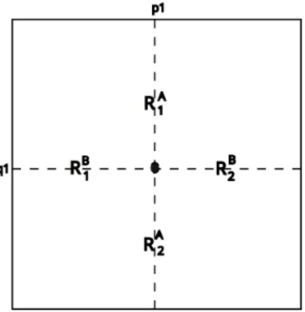
The sets ⌃Aand ⌃Bcan be partitioned, respectively, into n and m parts.
RBj as the preference region of strategy j for player B. In other words we can say that the region RB
j is a set of strategies of player A (belongs to ⌃A) to
which the best response of player B is strategy j. This means, the strategy j is the one where B expects to get the highest payo↵ when A chooses to play a strategy in RB j . ( RA i := BRA1(ei)✓ ⌃B for i = 1, ..., m RBj := BRB1(ej)✓ ⌃A for j = 1, ..., n
We use the notation Rij := RBj ⇥ RAi for j = 1, ..., n and i = 1, ..., m for the
subsets of ⌃ when A and B have a fixed strategy preference.
Definition 3. For a generic game (A, B) a codimension-one hyperplane of ⌃A is a subset of ⌃A where BRB contains two di↵erent pure strategies ej
and ej0 and all respective convex combinations. To these hyperplanes we
call indi↵erence sets and we represent them as ZjjB0. The same happens for
ZiiA0. The formal definition is
ZiiA0 := q2 ⌃B: (Aq)i = (Aq)i0 (Aq)k8k = 1, ..., m
ZjjB0 := n p2 ⌃A: (pB)j = (pB)j0 (pB)l8l = 1, ..., n o or equivalently, ZiiA0 = RiA\ RAi0 ✓ ⌃B and ZjjB0 = RBj \ RBj0 ✓ ⌃A for i6= i0 and j6= j0.
Interpreting this mathematical terminology, ZB
jj0 is a subset of ⌃A
form-ing the boundary of two distinct regions RB
j and RBj0. For player B, when
A chooses to play a strategy p placed in this border subset, is indi↵erent to choose strategy j or j0. Both of them give him the same utility and that utility is the maximum utility he achieves in response to strategy p of A. Definition 4. A (mixed) strategy profile (¯p, ¯q) 2 ⌃ is called a Nash equi-librium, if
¯
p2 BRA(¯q) and ¯q2 BRB(¯p)
If a Nash equilibrium lies inside ⌃, it is called completely mixed, otherwise it is called pure.
This notion was firstly introduced by John Nash in 1950. To better understand the behaviour of the players. (see Jr. (1951))
The main idea of this concept is that, in Nash equilibrium the optimal outcome of a game is one where no player has a motivation to deviate from his chosen strategy after considering a rival’s choice. In general, an indi-vidual can receive no incremental benefit from changing actions, assuming other players remain constant in their strategies.
Suppose that player A pick the strategy i and player B choose strategy j. We say that the pair (i, j) is a Nash Equilibrium if and only if i is the best response to j and simultaneously j is the best response to i. When this happens, neither player has motivation to switch to a di↵erent strategy. Note that this doesn’t mean that both players are getting the highest possible payo↵. This means that they are both receiving the highest possible payo↵ given their opponent’s strategy.
The Nash equilibrium may be not unique. The set of Nash equilibrium may consists of discrete or continuous points in ⌃.
It was proved also by Nash (see Jr. (1951)) that the set of Nash equilib-rium is non-empty for every bimatrix game. The proof of the existence of a Nash equilibrium is a classical application of Kakutani fixed point Theorem for correspondences (see Ok (2007))
The following lemma gives a simple characterization of a completely mixed Nash equilibrium. Its proof can be found in Osborne (2003).
Lemma 1. The point EA, EB 2 int (⌃) is a (completely mixed) Nash equilibrium of an m⇥ n bimatrix game (A, B) if and only if, for all i, i0 =
1, ..., m and j, j0 = 1, ..., n,
AEB i= AEB i0 and EAB j = EAB j0
This Lemma says that when B plays the strategy EB, player A gets the same payo↵ whatever strategy he uses. The same happens to player B when A plays EA. Summing up, in response to EB, player A is indi↵erent between all his strategies and similarly player B is also indi↵erent between all his strategies when A chooses play EA. This Lemma also ensures that EA2 RB j
and EB 2 RAi for all i, j. So, (EA, EB) 2 Rij and EA 2 ZjjB0, EB 2 ZiiA0
for all i, i0, j, j0. Geometrically, this Lemma represents the intersection of all indi↵erence regions.
Example 1 (Prisoners Dilemma). Two prisoners (A and B), suspected of theft, are taken into custody. However, cops don’t have enough evidence to sentence them of that crime but only to sentence them on the charge of possession of stolen goods.
The cop will examine their answers on separate rooms, this means that the prisoners can’t talk to each other (so we are in the presence of imperfect information). Each one of them has two possible answers, they can lie or confess. In the first one they are cooperating to each other saying that they don’t stole the goods, in the second one they assume the crime. We can find four possible cases. First, if they cooperate with each other, this means that none of them confesses the crime (Lie,Lie), they will both be charged the lesser sentence, a year of prison each. Second possible situation is when both prisoners confess the crime, in this case each prisoner will be sentenced to two years. The third and fourth situation is when one of them confesses the crime and the other one does not. The cop wants that each of the prisoners confess the crime, for this he o↵ers them an incentive, a ’get out of jail free card’, while the other prisoner that doesn’t confess will be sentenced to a three years term.
Both of them receives the same deal and they know the consequences of each action. They know also that the other prisoner receives the same conditions, we say that we have complete information. Since two players cannot contact with each other and assuming that they will make the deci-sion at the same time, this game can be considered as a simultaneous game, and can be analysed using the strategic form, looking to the correspondent bimatrix, which synthesized the four possible situations.
Prisoner B Prisoner A 0 B B B B B B @ Lie Conf Lie 1y 1y 0y 3y Conf 3y 0y 2y 2y 1 C C C C C C A
Interpreting this bimatrix we can check the four cases described before. So, if neither of them confesses (Lie,Lie), they will be penalized one year each. If both players confess the crime (Confess,Confess), they will be pe-nalized a two years sentence each. In the other hand, if only one confesses (Lie,Confess) or (Confess,Lie), the prisoner who confesses will go free, while the other will be penalized a three years sentence. These can be seen as the respective payo↵ for each set of strategies.
As we said before, in order to solve this problem each prisoner will evalu-ate their best strevalu-ategy according to their own benefit taking into account the
other prisoner’s possible strategies. Obviously, they have a greater benefit the less years they are in jail. By eliminating all dominated strategies, we can get the dominant strategy.
Before thinking about what each player is going to do in this situation, let us present the individual payo↵ matrix for each one of the players.
We get for player A and B, respectively, A = 1 3 0 2 , B = 1 0 3 2
For choosing his best strategy, player A has to have in consideration the choice of player B. So he has to build a belief about what strategy player B is going to make. Looking at the payo↵ matrix of player A we see that if player B lies (first column,
1
0 ), A stays better, this means, maximizes your own payo↵, if he plays ”confess”. Since if he lies he would be arrested one year instead of remaining free. In the other hand, if B confesses (corresponds to second column,
3
2 ), prisoner A will choose confess, because with that choice he gets stuck two years instead of three, what would happen if he lies. Given this, we can conclude that the best response for player A is always confess, regardless of which strategy B chooses.
We can apply the same logic to player B, looking at his payo↵ matrix. If A lies, the best response of B will be confess and if A confesses the best response of B will be confess as well. So, the rational thing to do for player B is also to confess.
Therefore, ’to confess’ is the dominant strategy. Since, (Confess, Con-fess) is the set of strategies that maximises each prisoner’s utility given the other prisoner’s strategy. It is the Nash Equilibrium of this game.
But here is the dilemma. As we seen before, Nash Equilibrium can be used to anticipate the result of the finite games, whenever such equilibrium exists. Both prisoners are choosing to protect themselves at the expense of the other participant, but as a result of this purely logical thought process, in the end we will face with a situation where the two players find themselves in a worse state than if they had cooperated with each other in the decision-making process. Here the Nash Equilibrium does not meet the criteria for being Pareto optimal. In other words, the individual choice of each one of the players is to lie. As we have seen, when this happens both of them get stuck for two years. However, this is not the best joint option because if the two players confess, they only get stuck one year each instead of two.
The prisoner’s dilemma is an abstraction of common situations where the choice of the best individual leads to both of them confess down, whereas if they both lying they would provide better results. It is said that this dilemma has an ’inefficient balance’ because the scheme of incentives and rationality leads to worse results.
Sometimes it is not so simple to find out the Nash equilibrium, (p⇤, q⇤). Therefore, we will show how to get it analytically.
Considering that p⇤ is the best response of player A, whatever B0s move, and q⇤ is the best response of B, whatever A plays, thus we have,
p⇤2 BRA(q⇤) and q⇤ 2 BRB(p⇤)
To find the Nash Equilibrium, first we have to computeBRA andBRB.
Let us deduce the explicit expression for both of them. BRA(q) = arg max
p (pAq) = arg maxp
⇥ p1 p2⇤ 1 3 0 2 q1 q2 = = arg max p ( p1q1 (3p1+ 2p2) q2) = = arg max p ( p1 2 + 2q1)
Knowing that p12 [0, 1], whatever q1, the p1 that maximizes the last result
is p1 = 0. As p1+ p2 = 1, p2= 1 and so, p = (0, 1), that is,BRA(q) = (0, 1).
Applying the same reasoning to player B we getBRB(p) = (0, 1)
In this example we are in the presence of a constant Best Response function. Hence we have,
⇢ (0, 1)2 BRA((0, 1)) (0, 1)2 BRB((0, 1)) ) ⇢ p⇤ = (0, 1) q⇤ = (0, 1)
Therefore, the Nash Equilibrium of the game is (Confess, Confess).
Recalling that RAi , i = 1, 2 is the preference region of strategy i for player A, this is, the set of strategies of B to which A best response is i. So, we have RA
1 and RA2 ✓ ⌃B. Similarly to player B where RB1 and R2B ✓ ⌃A.
Given this and the definition on preference region given before, we are able to compute the preference regions of strategies 1 and 2 and the corre-sponding indi↵erent sets for each one of the players,
RA1 =BRA1(e1) =?, RB1 =BRB1(e1) =?
RA2 =BRA1(e2) = ⌃B, RB2 =BRB1(e2) = ⌃A
and ZA
Example 2 (Matched Pennies Game). Sometimes there’s no pure Nash equilibrium at all. This example is one such case. In these cases we make predictions about players behaviour. Considering that they may behave randomly, we enlarge the set of strategies to include the possibility of ran-domization. Even in these cases, as John Nash conclude, the equilibria always exist.
Matching Pennies is a zero-sum game in that one player’s gain is the other’s loss. It is played between two players, A and B. Each one of them has a coin labelled with a head (H) and a tail (T). Each player should turn the coin and check if it became head or tail. Then, simultaneously, they reveal the result to each other. If the result match, this means, both are heads or both are tails, player A wins and keeps both coins. In this scenario, A gets the player B coin, so he wins +1 and B losses his coin, this means he gets 1. Otherwise, if the result do not match (one is head and other one is tail) player B keeps both coins. So, he gets +1 and player A gets 1.
We can illustrate the game in a payo↵ matrix, where in each cell we have the correspondent payo↵ for each player.
player B player A 0 B B B B B @ H T H 1 +1 +1 1 T +1 1 1 +1 1 C C C C C A The individual payo↵ matrices are,
A = +1 1 1 +1 , B = 1 +1 +1 1
Looking at the individual payo↵s matrices we can verify that if player B chooses Head, A gets better choosing Head too. However, if B plays Tail, A chooses Tail as well. The same happens with player B. If A picks Head, B will choose Tail in order to maximize their own payo↵. But if A plays Tail, B gets better with Head.
As we can see, in this game there’s no pure strategy Nash equilibrium, since there is no pair of strategies (heads or tails) that are best responses to each other. For any pair of strategies, one of the players wants to change what they are doing. In this situation we shouldn’t consider simply the
strategies H and T, but also the mixed strategies. If no equilibrium exists in pure strategies, one must exist in mixed strategies. Mixed strategy is a probability distribution over two or more pure strategies. When we do this we are introducing randomized behaviour, this means that each player is not choosing a particular choice between H and T but rather is choosing the probability which he will play H or T.
Therefore, the possible strategies for both players are numbers between 0 and 1. Let us consider p1 2 [0, 1] the probability of player A plays Head,
so (1 p1) 2 [0, 1] is the probability of player A plays Tail. Similarly for
player B, q1 2 [0, 1] is the probability which he chooses to play Head and
(1 q1)2 [0, 1] is the probability which he plays Tail.
Now, each player do not have only two possible strategies but rather a set of strategies corresponding to the interval of numbers between 0 and 1. This is what we call mixed strategies.
To find the Nash Equilibrium, just as we did for the Prisoner’s example, we will compute firstBRA andBRB.
BRA(q) = arg max p ⇥ p1 1 p1⇤ 1 1 1 1 q1 1 q1 = = arg max p (2p1(2q1 1) 2q1+ 1) = arg max p ((2p1 1) (2q1 1))
We want to maximize ((2p1 1) (2q1 1)) with respect to p1. When
q1 12 the expression (2q1 1) is positive and the p1 that maximizesBRA
is p1 = 1. On the other hand, when q1 12 we have (2q1 1) < 0 and the
maximum is reached when p1 = 0. Summing up, player A chooses to play
H, this means, BRA(q) = (1, 0), when q1 12 and he prefers to play T,
BRA(q) = (0, 1), when q1 12. If q1 = 12 he is indi↵erent between plays H
and T. In that case the best response is any p1 2 (0, 1).
Analogously, we can compute BRB(p). After some calculations, we get
that if p1 12 the strategy q1 that maximizes BRB is q1 = 0. This is
player B prefers T instead of H and so, BRB(p) = (0, 1) = e2. When
p1 12, the maximum is obtained if he chooses to play H, q1 = 1, and
BRB(p) = (1, 0) = e1. In the case where p1 = 12 he is indi↵erent between
all his possible strategies. Therefore, we get BRA(q) = ⇢ (1, 0) , q1 12 (0, 1) , q1 12 , BRB(p) = ⇢ (0, 1) , p1 12 (1, 0) , p1 12
Preference Region of strategy 1 for player A : R1A=BRA1(e1) =BRA1((1, 0)) =
⇢
(q1, q2) : q1 1
2 Preference Region of strategy 2 for player A :
R2A=BRA1(e2) =BRA1((0, 1)) =
⇢
(q1, q2) : q1
1 2 Preference Region of strategy 1 for player B :
RB1 =BRB1(e1) =BRB1((1, 0)) =
⇢
(p1, p2) : p1
1 2 Preference Region of strategy 2 for player B :
RB2 =BRB1(e2) =BRB1((0, 1)) =
⇢
(p1, p2) : p1 1
2 The indi↵erence sets, ZA
ii0 and ZjjB0 are Z12A = RA1 \ RA2 = ✓ 1 2, 1 2 ◆ and Z12B = RB1 \ R2B= ✓ 1 2, 1 2 ◆
By Lemma 1, the game has a mixed Nash Equilibrium 12,12 . See Figure A.1.
Chapter 3
Fictitious Play Dynamics
In this chapter we will introduce some basic notions about dynamical system modelling the repeated or continuous play of a game, in other words, we will define the fictitious play (FP). This type of games is based on the following rule:
At each stage of the game, each player determines the (mixed) average strategy of him opponent’s play up to this time and plays a (pure) best re-sponse to it.
Recall that ⌃ = ⌃A⇥ ⌃B is the space of mixed strategy profiles where
the dynamical system of fictitious play is defined and under the hypothesis that the players follow a stationary strategy distribution along entire game. Fictitious play is an algorithm seen as the dynamics beliefs of the opponent about the player’s strategy distribution.
Often the fictitious play algorithm is called myopic learning rule. This happens because players ambition at maximize the next-round payo↵ looking only for the past of the play. They do not try to produce any extra strategic considerations to a↵ect their opponent’s future behaviour.
Fictitious Play has two versions: discrete-time and continuous-time. Both of them were present by Brown in 1951 (see Brown (1951)).
In the beginning, the discrete version was more famous, designed to be an algorithm for numerical approximation of Nash equilibrium in zero-sum games. This happened due to the work of Robinson in 1951 (see Robinson. (1951)) where he showed that the process converges to Nash Equilibrium in zero-sum games. To more detail about discrete-time process see also Berger (2007)
In present chapter we will defining both, discrete and continuous time versions. (see Ostrovski (2013))
3.1
Discrete-time fictitious play
As usual, consider two players, A and B. Let (A, B) be an m⇥ n bimatrix games. The strategy set for player A is SA and for player B, SB. They
play repeatedly at times k 2 N0. Assume that (xk, yk) 2 SA⇥ SB denote
the (pure) strategies chosen by the players at time k 2 N, with an initial condition (x0, y0)2 ⌃.
For k2 N, we can compute pk:= 1 k k 1 X i=0 xi 2 ⌃A and qk:= 1 k k 1 X i=0 yi 2 ⌃B
where pk and qk are the empirical average play through time k 1.
The fictitious play rule, presented in the beginning of this chapter, re-quires that,
xk2 BRA(qk)\ SAand yk2 BRB(pk)\ SB (3.1)
for all times k2 N
We can also describe pkand qkas the beliefs of the two players, A and B,
about the strategy distribution of respective their opponent. By definition, we are able to calculate the set where pk+1 and qk+1 belong
pk+1= 1 k + 1 k X i=0 xi = 1 k + 1xk+ k k + 1 1 k k 1 X i=0 xi = 1 k + 1xk+ k k + 1pk 2 1 k + 1BRA(qk) + k k + 1pk = 1 k + 1(BRA(qk) + kpk) Equivalently, qk+1 2 1 k + 1BRB(pk) + k k + 1qk
Definition 5. For a bimatrix game (A, B) with mixed strategy space ⌃, discrete-time fictitious play is the process (pk, qk) 2 ⌃, k 1, given by the
initial condition (p1, q1)2 ⌃ and for k 1,
pk+12 1 k + 1(BRA(qk) + kpk) (3.2) qk+12 1 k + 1(BRB(pk) + kqk) (3.3) Remark 1. Geometrically, when players A and B have beliefs (pk, qk) 2
Rij ⇢ ⌃ or, in other words, their best responses to the opponent’s play are i
and j, respectively, then pk+1 is in the line segment between pk and ei2 ⌃A
and the same happens to qk+1, which will lies on the line segment between qk
and ej 2 ⌃B. So, we can say that both players’ beliefs (pk, qk) move towards
their currently preferred pure strategy, with step size decreasing with time k. Remark 2. Notice that,
pk+1 pk= 1 k + 1 k X i=0 xi pk = 1 k + 1xk+ k k + 1 1 k k 1 X i=0 xi pk = 1 k + 1xk+ k k + 1pk pk 2 1 k + 1BRA(qk) + k k + 1pk pk = 1 k + 1(BRA(qk) + kpk (k + 1) pk) = 1 k + 1(BRA(qk) pk) and, qk+1 qk2 1 k + 1(BRB(pk) qk) In order thatkpk+1 pkk and kqk+1 qkk are bounded by
p 2
(k+1). This means
that the step size of fictitious play decreases like 1k. This express the fact that new data about the opponent has decreasing impact as k grow.
3.2
Continuous-time fictitious play
In this section we will assume a continuous-time process, instead of a game that are played again and again.
A continuous-time fictitious play is seen as a dynamical system where players are presumed to continuously play a given bimatrix game by choosing the best response to the average of their respective opponent’s past play at each time t > 0 (see Hofbauer & Sigmund (1998)).
Formalizing this notion mathematically we have that p (t) = 1 t Z t 0 BRA (q (s)) ds, tp (t) = Z t 0 BRA (q (s)) ds Deriving both sides in order to t, we get
p (t) + tp0(t) =BRA(q (t)), p0(t) =
1
t(BRA(q (t)) p (t))
Given this and doing a parallel with discrete-time studied in last section, we give the following definition.
Definition 6. For a bimatrix game (A, B) with mixed strategy space ⌃, continuous-time fictitious play is the process (p (t) , q (t)) 2 ⌃, t t0 > 0,
given by the di↵erential incluision ˙p (t)2 1
t (BRA(q (t)) p (t)) and ˙q (t)2 1
t (BRB(p (t)) q (t)) considering some initial condition (p (t0) , q (t0)) = (p0, q0)2 ⌃.
Remark 3. (1) Based on last definition we note that fictitious play is a di↵erential inclusion. We cannot ensure the uniqueness of solutions. How-ever, by general theory, we can ensure that solutions exist for all initial conditions. This conclusion is due to the fact thatBRA andBRB are upper
semi-continuous correspondences with closed and convex values (faces of ⌃A and ⌃B) (see Aubin & Cellina. (1948))
(2) We can even conclude that Nash equilibrium are precisely the equilib-rium of fictitious play dynamics FP. Particularly, if an orbit of FP converges to a single point, that point is a Nash equilibrium.
(3) As we have seen before, in discrete-time case, BRA and BRB are
piecewise constant on the convex sets RB
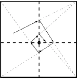
Based on this fact we can check that orbits are locally straight line segments going for vertices of ⌃. They just alter their trajectory direction when they hit on an indi↵erence set, in order words, when they change the block Rij.
(next figure is an example of what happen in case 2⇥ 2 games)
Figure 3.1: Trajectory over time
(4) As we see in last definition, Fictitious Play is time-dependent. How-ever, if we make a change of variable in time, we can turns it into an autonomous system. We can assume that without loss of generality because the time dependence is related with the slowing down of the motion as time progresses and no related with the actual shape of the trajectories.
So, considering that t = e⌧ and so ˜p (⌧ ) = p (e⌧) and ˜q (⌧ ) = q (e⌧) we get, @ ˜p @⌧ = @p @t(e ⌧)@ (e⌧) @⌧ = p 0(e⌧) e⌧ = 1 e⌧ (BRA(q (e ⌧)) p (e⌧)) e⌧ = =BRA(q (e⌧)) p (e⌧) Therefore, ˜ p0(⌧ ) =BRA(˜q (⌧ )) p (⌧ )˜
Now we can think about FP as an autonomous system. This will simplify certain arguments. We can give, now a formal definition for this system (see Hofbauer & Sigmund (1998)).
Definition 7. For a bimatrix game (A, B) with mixed strategy space ⌃, best response dynamics (BR) is the process (p (t) , q (t))2 ⌃, t 0, given by the di↵erential inclusion,
˙p (t)2 BRA(q (t)) p (t) and ˙q (t)2 BRB(p (t)) q (t)
We will denote by x(t), x : [0,1) ! ⌃A the strategy played by player A
and y(t), y : [0,1) ! ⌃B by player B, at time t > 0.
Example 3 (Prisoner’s Dilemma cont.). Let us apply these concepts to the example of the prisoners dilemma presented in the last chapter. Now, we are supposing that players want their strategies evolve over the time. Notice that
⌃A= ⌃B= (x1, x2)2 R2+: x1+ x2= 1
According to the definition of Fictitious Play, strategies p and q evolve ac-cording to the equations
⇢
˙p =BRA(q) p
˙q =BRB(p) q
Implement this in Prisoner’s Dilemma we get ⇢ ˙p = (0, 1) (p1, p2) ˙q = (0, 1) (q1, q2) , ⇢ ( ˙p1, ˙p2) = ( p1, 1 p2) ( ˙q1, ˙q2) = ( q1, 1 q2)
Solving this system of ODEs we obtain the following results 8 > > < > > : p1(t) = e tp1(0) p2(t) = 1 e tp1(0) q1(t) = e tq1(0) q2(t) = 1 e tq1(0)
We can even check that over time the solution will moves towards the best response
lim
t!1p (t) = limt!1(p1(t) , p2(t)) = (0, 1) , limt!1q (t) = limt!1(q1(t) , q2(t)) = (0, 1)
Dynamics of ODE can be sketch in the following phase portrait. (see Figure A.2). It is generated by a product of two intervals 1A⇥ 1
B =
[0, 1]⇥ [0, 1], each one correspondent to strategies interval for p1 and q1,
respectively. Note that strategies p2 and q2 can be obtained at the expense
of p1 and q1, respectively.
3.3
Uniqueness of fictitious play flow
As we said before, whatever it is the initial condition (p0, q0) 2 ⌃, the
continuity of the flow induced by this system is not so true. It just holds for generic bimatrix games and not for all.
The problem happens when the solution curves crosses any one of the indi↵erence sets ZA =Si,i0ZiiA0 or ZB=
S
j,j0ZjjB0. In these sets, the
right-hand sides are multi-valued and that can provide non-uniqueness of solu-tions. Locally we do not have these problems. In fact, in the interior of the convex sets Rij ✓ ⌃, the solutions of FP are unique and continuous and the
segments are straight lines. To work around this problem, all of ZiiA0 and ZjjB0
are required to be codimension-one planes and that the flow crosses them transversally. It follows a proposition.
Proposition 1. (see Sparrow (2008)) Let (A, B) be an m⇥ n bimatrix game. Denote Z⇤= ZB⇥ ZA the set where each of the players is indi↵erent
between at least two strategies. Assume that for all (p, q)2 ⌃\Z⇤, if p2 ZB
and q /2 ZA so that, say, BR
A(q) = ek, then ek is not parallel to the plane
ZB ⇢ ⌃A at the point p, and similarly for the roles of p and q reversed.
Then FP defines a continuous flow on ⌃\ Z⇤.
After a more detailed analysis about the set Z⇤ it is possible to obtain a stronger result. To get more detail about this see Sparrow (2008).
Proposition 2. Assume the bimatrix game (A, B) satisfies the hypotheses of last proposition and additionally assume that A and B have maximal rank. Then the flow on the interior of the sets Rij has a unique continuous
extension everywhere (on ⌃), except possibly points in the subset of Z⇤where one of the players is indi↵erent between at least three of his strategies. This remaining set has a codimension three.
Chapter 4
Analysis of 2
⇥ 2 Fictitious
Play
One of the earliest conclusions in game theory was that in any 2⇥2 bimatrix game all solutions of Fictitious Play converge to a point, the Nash equilib-rium point. Miyasawa (see Miyasawa (1961)) give us the first proof of this result. Later Metrick and Polack (see Metrick & Polak (1994)) present a more conceptual and geometric proof.
Theorem 1 (Miyasawa, Metrick and Polak). For any 2⇥ 2 bimatrix game (A, B), any orbit{(p (t) , q (t)) , t t0} of FP with initial condition (p (t0) , q (t0)) =
(p0, q0)2 ⌃ for some t0 0 converges to a Nash equilibrium (p⇤, q⇤)2 ⌃ as
t! 1.
In this chapter we will analyse all the possible types of phase portraits arising in 2⇥ 2 fictitious play.
4.1
Indi↵erence sets
As we already said, for generic values of p and q, BRA and BRB are in
general a pure strategy. But in fact, that is not always true. As we have seen, when we are looking at the indi↵erence sets the best response consists in more than one pure strategy. In these sets we face with e1Aq = e2Aq
or pBe1 = pBe2 for player A and B, respectively. This means that both of
pure strategies, e1 and e2, provide the same utility to the players.
Therefore, also any convex combination between e1 and e2 gives to A
4.1.1 Identification of the indi↵erence sets
In the present section we will show you how to explicitly identify indi↵erence sets, ZijA and ZijB. For better understand the dynamics of this we will first present you a generic 2⇥ 2 case.
For player A, consider that aij is his pay-o↵ when he chooses the strategy
i given that player B played j. The pay-o↵ matrix for player A is A =
a11 a12
a21 a22
Remember that, q1+ q2= 1, e1 = (0, 1) and e2= (1, 0). Developing the
definition of indi↵erence set we get : e1Aq = e2Aq, ,⇥0 1⇤ a11 a12 a21 a22 q1 q2 = ⇥ 1 0⇤ a11 a12 a21 a22 q1 q2 , , q1 = (a22 a12) (a11 a21) (a22 a12) , , q1 = 1 (a11 a21) (a22 a12)+ 1
Looking at this result we are able to say that, in the case 2⇥ 2 fictitious games, the indi↵erence set is just a point. Denote this point by q1⇤. We know that q1 2 (0, 1), so even q⇤1. In order for q⇤1 2 (0, 1) we need to ensure that
A=
(a11 a21)
(a22 a12)
0
For player B, using the same principles we will compute ZijB. Let the pay-o↵ matrix for player B be
B =
b11 b12
b21 b22
indi↵erence set of B pBe1 = pBe2. pBe1= pBe2, ,⇥p1 p2⇤ b11 b12 b21 b22 1 0 = ⇥ p1 p2⇤ b11 b12 b21 b22 0 1 , ,⇥p1b11+ p2b21 p1b12+ p2b22⇤ 1 0 = ⇥ p1b11+ p2b21 p1b12+ p2b22⇤ 0 1 , , p1 = 1 (b11 b12) (b22 b21)+ 1
Using the same notations that we use for player A, let us denote the point p1 of indi↵erence set by p⇤1. We know that p⇤1 2 (0, 1) so we have to
certify that
B =
(b11 b12)
(b22 b21)
0
Definition 8. We say that player A is independent from player B moves if Z12A =?. Similarly, B is independent from A choices if Z12B =?
In other words, saying that A is independent from B is the same as saying that player A does not change his strategy regardless of B0s choice. Given this, player A has no indi↵erence sets.
Lemma 2. player A is not independent from player B moves, if and only if,
A=
(a11 a21)
(a22 a12)
> 0 This implies that q1⇤2 (0, 1) and so ZA
12 is not empty.
Analogously, player B is not independent from A if and only if,
B =
(b11 b12)
(b22 b21)
0 Which means that p⇤1 2 (0, 1) and so ZB
12 is not empty. Remark 4. Moreover, if (q⇤1, q2⇤)2 ZA 12 then q⇤1 = 1 A+ 1 Equivalently, if (p⇤1, p⇤2)2 ZB 12 then p⇤1 = 1 B+ 1
Example 4 (Simple example). Consider player A pay-o↵ matrix, A =
2 1 1 2
Lets compute the value of
A=
(a11 a21)
(a22 a12)
= 2 1
2 1 = 1 > 0
Consequently, A is not independent from B and q1⇤ = 1+11 = 12. We are also able to compute the value of q2⇤ = 1 q1⇤ = 1 12 = 12. Thus, as we said before, the indi↵erence set corresponds to a point ZA
12= (12,12) .
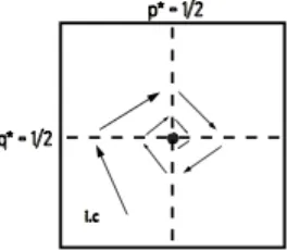
The point q⇤ = (12,12) is the strategy of B for which A is completely indi↵erent to play e1or e2. We can see this graphic representation in Figure
A.3.
If player B chooses a strategy q located in Z1 we getBRA(q) = e1. On
the other hand, if B q is in Z2,BRA(q) = e2. As we had already conclude,
in the graphic we can certify that A is not independent from B0s choices since he changes his best strategy depending on B. His strategy depends where q is posted.
In the previous paragraph we assume that if q2 Z1 A chooses strategy
e1 and if q2 Z2 A prefer e2. But how can we know that ?
First we assume that player B plays e2 this is, q = (0, 1). Now we will
computeBRA(e2) to check which strategy gives to A the largest pay-o↵ in
response to B choice. • If A plays e1 : e1Aq = e1 a11 a12 a21 a22 e2= ⇥ 1 0⇤ 2 1 1 2 0 1 = ⇥ 2 1⇤ 0 1 = 1 • If A plays e2 : e2Aq = e2 a11 a12 a21 a22 e2= ⇥ 0 1⇤ 2 1 1 2 0 1 = ⇥ 1 2⇤ 0 1 = 2
As 2 > 1, when B picks e2, player A gets higher pay-o↵ if he chooses e2
too. Since e22 Z2 we can assume that in that region A will answer with e2
in order to maximize his utility.
Using the same reasoning, we can check what happens when player B picks e1. We will reach the conclusion that player A will prefer e1in response
to e1 played by B. So, in region Z1 player A will be more satisfied if he
Now, we will see, in the general case, how can we know the best response of A for a given pure strategy played by B.
First we assume that B plays q = e2 = (0, 1). Let’s figure out which is
the best response of player A. 8 > > < > > : e1Ae2= e1 a11 a12 a21 a22 e2 = a12, A plays e1 e2Ae2= e2 a11 a12 a21 a22 e2 = a22, A plays e2
Therefore, we just need to compare the values of a12and a22 in order to
know the preferences of player A in response to player B choice e2.
• If a22> a12 we get BRA(q) = ⇢ e2, q2> q⇤2 e1, q2< q⇤2 = ⇢ e2, q1< q⇤1 e1, q1> q⇤1 • If a12> a22, we obtain BRA(q) = ⇢ e1, q2> q⇤2 e2, q2< q⇤2 = ⇢ e1, q1< q⇤1 e2, q1> q⇤1
Analogously, assuming that player B play e1, this means that, q = (1, 0)
we get 8 > > < > > : e1Ae1= e1 a11 a12 a21 a22 e1 = a11, A plays e1 e2Ae1= e2 a11 a12 a21 a22 e1 = a21, A plays e2
In this case we just have to confront the values of a11and a21to find out
the best option for player A.
If a11 > a21 player A prefer to play e1. In the other hand, if a11< a21
player A gets more utility if he chooses e2. Summarize,
• When a11> a21
BRA(q) =
⇢
e1, q1> q⇤1
e2, q1< q⇤1
• In the other hand, when a11< a21
BRA(q) =
⇢
e1, q1< q⇤1
Proposition 3. We can summing up these 4 cases.
BRA(q) =
⇢
e1, (q1> q1⇤^ a11> a21)_ (q1 < q1⇤^ a12> a22)
e2, (q1> q1⇤^ a11< a21)_ (q1 < q1⇤^ a12< a22)
Doing the same analysis for player B, this is, assuming that player A plays his pure strategies, p = e1 or p = e2, we will compute the best
re-sponses of B.
We will apply exactly the same procedure as we did before. First assum-ing that A plays p = e2= (0, 1).
8 > > < > > : e2Be1= e2 b11 b12 b21 b22 e1= b21, B plays e1 e2Be2= e2 b11 b12 b21 b22 e2= b22, B plays e2
Concluding we just have to contrast the values of b21 and b22 to get the
best response of B when A plays e2. If b21 > b22 B gets more utility if he
plays e1. On the other hand, when b21< b22 B prefers the strategy e2.
Consider now that player A plays p = e1 = (1, 0).
8 > > < > > : e1Be1= e1 b11 b12 b21 b22 e1= b11, B plays e1 e1Be2= e1 b11 b12 b21 b22 e2= b12, B plays e2
In this case we will compare the values of b11and b12. If b11> b12player
B will take the strategy e1. However, if b11< b12 he opts by e2.
Just as we do for player A let’s summing up these 4 results in a propo-sition. Proposition 4. BRB(p) = ⇢ e1, (p1> p⇤1^ b11> b12)_ (p1 < p⇤1^ b21> b22) e2, (p1> p⇤1^ b11< b12)_ (p1 < p⇤1^ b21< b22)
Now let us study and apply these concepts in another example of 2⇥ 2 fictitious play.
4.1.2 Examples
Example 5 (A not independent from B but B independent from A). Con-sider the pay-o↵ matrices for player A and B respectively,
A = 3 1 1 2 B = 0 1 1 2
In order to know the indi↵erence sets, we will compute the values of A
and B, A= (a11 a21) (a22 a12) = 3 1 2 1 = 2 > 0 and B = (b11 b12) (b22 b21) = 0 1 2 1 = 1 < 0
For player A we have that Z12A 6= ? and q⇤1 = 2+11 = 31, q2⇤= 1 q1⇤ = 23. And so ZA
12= 13,23
Although for player B, Z12B = ?. This means that player B is inde-pendent from A and therefore he has only one strategy that maximizes his pay-o↵ whatever the A plays.
In this case our scenario is, • A is not independent from B • B is independent from A
The next step is to analyse the phase portrait for this scenario where we have a strategy q⇤ of B that divides the best responses of A, but we don’t have the strategy p⇤.
To player A we have a22 = 2 and a12 = 1, so a22 > a12, therefore (See
Figure A.4) BRA(q) = ⇢ e2, q1 q⇤1 e1, otherwise = ⇢ e2, q1 13 e1, otherwise
We already noticed the behaviour of player A. Now let us find the deport-ment of player B. As we saw, player B has just one best response whatever p is. Therefore, in order to know which one of pure strategies B prefer, we will assume that player A played e1 and verify how B reacts, if he gets higher
pay-o↵ using e1 or e2.
Next we will determine Nash equilibrium, (p, q) : p2 BRA(q) and q 2
BRB(p). Since B is independent from A, it is understandable thatBRB(p) =
e2, hence q = e2 for all values of p. Taking this into account, we are able to
identify theBRA(q),
BRA(q) =BRA(e2) =BRA((0, 1)) = e2, since q1 = 0
Summarizing, (p, q) = (e2, e2) and p = (0, 1) and q = (0, 1).
We can include this result in the Figure A.4, see Figure A.5.
The next step is to sketch the phase portrait of the associated fictitious play. Remember that p2 and q2 can be obtained from p1 and q1. Until here,
our analysis has been done in terms of p1 and q1 and for that reason we will
develop the next computations in these coordinates too. As we remember, 8 < : ˙p1 = ⇢ p1, q1 13 1 p1, otherwise ˙q1 = q1
We can automatically solve the second equation, ˙q1 = q1 , q1(t) = e tq1(0)
which is an asymptotically stable equilibrium. Whatever the initial condi-tion q1(0)2 (0, 1), q1 will always converges to zero. (See Figure A.6)
Conversely, in relation to p1 dynamics we need to take into account the
initial condition. We have two options for that, (1) q1(0)2 1 3, 1 and (2) q1(0)2 0,1 3
When the initial condition is (1) we are in the branch ˙p1 = 1 p1. In
this case, the trajectory has a tendency to converge in a straight line to one. So in the equilibrium we have p1 ! 1 and q1 ! 0. When the first condition
is localized in the button region, (2), we have ˙p1 = p1 the trajectory will
converges to zero. And so we have, p1 ! 0 and q1! 0. We are able now to
illustrate each situation graphically, see Figure A.7. Then we can join this two situations in only one graphic, see Figure A.8.
When the trajectory crosses the boundary region, in this specific case q1 = 13, changes its direction starting to converge to the equilibrium point
(p1, q1) = (0, 0), which is the Nash equilibrium.
In the last example we have analysed the scenario where A is not inde-pendent from B but, where’s B is indeinde-pendent from A. However this is not
the only possible case. Actually, we have four possible cases, 1. A is independent from B and B is independent from A 2. A is independent from B but B is not independent from A 3. A is not independent from B but B is independent from A 4. A is not independent from B and B is not independent from A Just as we did for case 3., we will now present three more examples for each one of the remaining cases.
Example 6 (A independent from B and B independent from A). Prisoner’s dilemma, the example that we have been developing throughout this work is an example of this first case. Remember the pay-o↵ matrices for player A and B,
A = 1 3 0 2 B = 1 0 3 2 Computing the values of A and B :
A= (a11 a21) (a22 a12) = 1 0 2 + 3 = 1 < 0 B= (b11 b12) (b22 b21) = 1 0 2 + 3 = 1 < 0
As we can see, both, Z12A and Z12B are an empty sets, so either player A is independent of player B as player B is independent of player A. In other words, regardless of the opponent’s move, both players have a unique strategy that maximizes their own pay-o↵.
Remember that in this specific example we have already computed the Nash equilibrium as well as the face portrait. See Figure A.2.
Until now, we had already seen first and third cases. About the second one we do not see as fundamental to develop an example here. The main idea is the same that we used for the third case. In this case, we just need to take into account that they are ’symmetric’ to each other and that in the second case we will get p⇤ as a vertical boundary region instead of q⇤ horizontal boundary region, obtained in example 5.
With respect to the forth case let us bring back the example of Matched Pennies.
Example 7 (A not independent from B and B not independent from A). Remember the pay-o↵ matrices of Matched Pennies game for each one of the players, A = +1 1 1 +1 , B = 1 +1 +1 1 Find the value of A and B,
A= (a11 a21) (a22 a12) = 1 ( 1) 1 ( 1) = 1 > 0 B= (b11 b12) (b22 b21) = ( 1) 1 ( 1) 1 = 1 > 0
So, we are in a presence of case four. Where both, player A and player B, depend on the opponent’s moves.
In this case we have Z12A 6= ? and Z12B 6= ?. Thus, we need to compute q⇤ and p⇤, q1⇤ = 1 1 + 1 = 1 2 ; q ⇤ 2 = 1 2 ) Z A 12= ✓ 1 2, 1 2 ◆ p⇤1 = 1 1 + 1 = 1 2 ; p ⇤ 2 = 1 2 ) Z B 12= ✓ 1 2, 1 2 ◆
So we have two strategies, q⇤ and p⇤ the first one divides the best responses of A into two parts and the second one divides the best responses of B also into two parts. We just already computed the Nash equilibrium for this example (check example 2). Just to remember we got
BRA(q) = ( (1, 0) , q1 12 (0, 1) , q1 12 , BRB(p) = ( (0, 1) , p1 12 (1, 0) , p1 12
And the Nash equilibrium found was (p1, q1) = 12,12
Let us now check the phase portrait.
˙ p1= ⇢ 1 p1, q1 12 p1, q1 12 , q˙1= ⇢ q1, p1 12 1 q1, p1 12
There are four possible of combinations between initial conditions of p1(0) and q1(0). See Figure A.9.
1. p1(0) 12 ^ q1(0) 12 : with this combination of initial
con-ditions we have ˙p1 = p1 and ˙q1 = 1 q1. Over time the trajectory will
converge to ˙p1! 0 and ˙q1 ! 1, this is the point (p1, q1) = (0, 1).
2. p1(0) 12 ^ q1(0) 12 : here we have ˙p1 = 1 p1 and
˙
q1 = 1 q1. Over time they will tend to ˙p1 ! 1 and ˙q1 ! 1 this is
the point (p1, q1) = (1, 1).
3. p1(0) 12 ^ q1(0) 12 : in this case we have ˙p1 = 1 p1 and
˙
q1 = q1. As time progresses the trajectory will run to ˙p1 ! 1 and ˙q1 ! 0
this means the point (p1, q1) = (1, 0).
4. p1(0) 12 ^ q1(0) 12 : the last combination is ˙p1 = p1 and
˙
q1 = q1. Here the path will evolve over time to ˙p1 ! 0 and ˙q1 ! 0, This
is, (p1, q1) = (0, 0).
4.1.3 Combinatorially distinct types
In accordance with the examples of last section we are now to show that fictitious play converges to Nash equilibrium (as claimed by Theorem 1) and the phase space belongs to a finite family of combinatorial distinct types. In this subsection we will synthesize all these types. Before we start, to simplify the notation, let, p, q2 [0, 1] denote the probability of player A and B, respectively.
As we saw in the last section, there is (p⇤, q⇤)2 R2, such that fictitious
play can be divided in four scenarios: (A) ˙p = ⇢ 1, q q⇤ 0, q q⇤ p and ˙q = ⇢ 1, p p⇤ 0, p p⇤ q (B) ˙p = ⇢ 1, q q⇤ 0, q q⇤ p and ˙q = ⇢ 1, p p⇤ 0, p p⇤ q (C) ˙p = ⇢ 1, q q⇤ 0, q q⇤ p and ˙q = ⇢ 1, p p⇤ 0, p p⇤ q (D) ˙p = ⇢ 1, q q⇤ 0, q q⇤ p and ˙q = ⇢ 1, p p⇤ 0, p p⇤ q
For each one of these four scenarios we will see what happen with the convergence when we change the values of p⇤ and q⇤. Changing these val-ues we are changing the independence relationship between players and also
changing the value of the Nash equilibrium. We found nine di↵erent combi-nations for p⇤ and q⇤. Let us see what happen for the case (A).
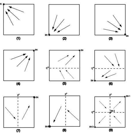
1. p⇤ 0 and q⇤ 1 we get ⇢
˙p = p
˙q = 1 q In this case we have that p is always greater or equal than p⇤ and q is always less or equal than q⇤. So, over time the trajectory will converge to the Nash equi-librium point which is (p, q) = (0, 1). We can see in the figure A.10 (1).
2. p⇤, q⇤ 1 we get ⇢
˙p = p
˙q = q Here, as in the previous case, q is always less or equal than q⇤, but in contrast with the last case p is also always less or equal than p⇤. Graphically, Figure A.10 (2), we can see that, over time the trajectory will converge to the Nash equilibrium point (p, q) = (0, 0).
3. p⇤ 1 and q⇤ 0 we get ⇢
˙p = 1 p
˙q = q . In this third case p p⇤ and q q⇤ so, over time, it will converge to the point (p, q) = (1, 0) which is the Nash equilibrium. See Figure A.10 (3).
4. p⇤, q⇤ 0 we get ⇢
˙p = 1 p
˙q = 1 q because p and q are always greater than p⇤ and q⇤, respectively, over time it will converge to the point (p, q) = (1, 1) which is the Nash equilibrium. See Figure A.10 (4). 5. 0 q⇤ 1 and p⇤ 0 we get ˙q = 1 q and so q will always
converge to 1. The convergence of p will depends on initial condition. However, as time goes by, it will always converge to the Nash equilib-rium point, which is (p, q) = (1, 1). We can check this in figure A.10 (5).
6. 0 q⇤ 1 and p⇤ 1, we get ˙q = q and so q will always
con-verge to 0. The concon-vergence of p will also depends on initial condition. Despite this, graphically we can prove that over time it will converge to the Nash equilibrium (p, q) = (0, 0) whatever it is the initial condition. Check the graph (6) in figure A.10.
7. 0 p⇤ 1 and q⇤ 0 we get ˙p = 1 p and so p will always
converge to 1. The convergence of q will change with the local of the initial condition but as time progress it will always converge to Nash point,(p, q) = (1, 1). See Figure A.10 (7).
8. 0 p⇤ 1 and q⇤ 1 here we get ˙p = p and so p will always
converge to 0. The convergence of q will change with the local of the initial condition. Once, graphically we check the convergence to the Nash equilibrium point, (p, q) = (0, 0). See Figure A.10 (8).
9. 0 q⇤ 1 and 0 p⇤ 1 in this last case the convergence will
depends on the initial condition of both variables. If p p⇤and q q⇤ we are in the first quadrant and the the trajectory will converge to the point (p, q) = (0, 0). If we are in the second quadrant, this is p p⇤ and q q⇤, the trajectory will converge to (p, q) = (0, 1) and go on.
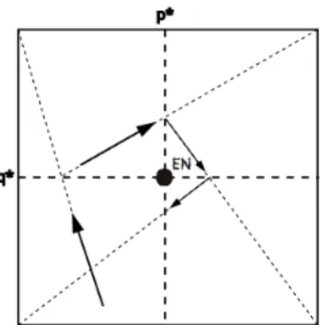
In the graphic (9) in figure A.10 we represent the three possible Nash equilibrium. We can check that the EN1 and EN3 are pure and stable. But EN2 are mixed and unstable.
We can use the same reasoning for the remaining three cases. We do not see as necessary to show all of them here because the idea is exactly the same used in case (A). However, we will develop the case 9,
0 q⇤ 1 and 0 p⇤ 1
for each one of the scenarios, since it is a compilation of all the other eight cases where none of the players is independent from the other.
(B) Here the trajectory is like an spiral and it will converge to the Nash equilibrium which is (p, q) = (p⇤, q⇤). This equilibrium is mixed and stable. Check Figure A.11.
(C) In this case the trajectory is symmetrical to scenario (B). The Nash equilibrium is either the mixed point, (p, q) = (p⇤, q⇤) and it is also stable. As we saw before, the Matched Pennies example is included in this scenario. See Figure A.12.
(D) Lastly, this scenario is the symmetric of scenario seen in case (A). There are two pure and stable equilibrium (EN1 and EN3) and one mixed and unstable equilibrium, EN2. See Figure A.13.
Chapter 5
Conclusions and Further
Research
In this dissertation we have studied a specific case of evolutionary games, the 2⇥ 2 fictitious play where we have two players both with two strategies. In case of zero-sum games, fictitious play always converge to a set of Nash equilibria. In our specific case study it was guaranteed, by Theorem 1, that the trajectories of the system always converge to the Nash equilibrium. Throughout this dissertation our main focus was to prove Theorem 1 and, show that the dynamics of 2⇥2 fictitious play is of finite type. In order to do that and to better understand this type of games we concentrated on the construction of an exhaustive list with all the possible combinatorially distinct types.
This study was done throughout chapter 4. Before that we clarified, from a dynamical point of view, the relation between the discrete and continuous fictitious play. These introductory and more theoretical chapters were the essential basis to achieve the main goal of this dissertation.
Based on this study we were able to present a family of examples of 2⇥2 fictitious play where we synthesized all the possible scenarios.
Regarding further research, a possible direction could be the study of games whose players have more than two pure strategies (see Sparrow (2008) and Shapley (1964)). For example the case where each one of the two players has three pure strategies. We know that, for these cases the convergence to the Nash equilibrium is not guaranteed. One of these cases is the example known as Shapley polygon where the fictitious play converges to a periodic orbit. Furthermore, it may not be possible to classify the dynamics with more than two pure strategies. In fact, in some games one may be in a
pres-ence of chaotic play. This opens a new area of study where many challenging problems are still waiting to be solved.
Bibliography
Aubin, J.-P. & Cellina., A. (1948), Di↵erential Inclusions, Springer.
Berger, U. (2007), ‘Brown’s original fictitious play’, Journal of Economic Theory .
Brown, G. W. (1951), Iterative solution games by Fictitious Play, Koopmans T.C. (Ed.), Activity Analysis of Production and Allocation.
Hofbauer, J. & Sigmund, K. (1998), Evolutionary games and population dynamics, Cambridge University Press, Cambridge.
Jr., J. F. N. (1951), Non-cooperative games, PhD thesis, Ann. of Math. Metrick, A. & Polak, B. (1994), ‘Fictitious play in 2 x 2 games: a geometric
proof of convergence’, Econom. Theory .
Miyasawa, K. (1961), On the convergence of the learning process in a 2 x 2 non-zero-sum two-person game, Econometric Research Program.
Morgenstern, O. & von Neumann., J. (1944), Theory of Games and Eco-nomic Behavior, Princeton University Press.
Ok, E. A. (2007), Real Analysis with Economic Applications, Princeton Uni-versity Press.
Osborne, M. J. (2003), Introduction to game theory, Oxford University Press. Ostrovski, G. (2013), Topics arising from Fictitious Play Dynamics, PhD
thesis, University of Warwick.
Robinson., J. (1951), An iterative method of solving a game, PhD thesis, Ann. of Math.
Shapley, L. (1964), Some topics in two-person games, Dresher, M., et al. (Eds.), Advances in Game Theory.
Sparrow, Colin, v. S. S. H. C. (2008), Fictitious play in 3-by-3 games: the transition between periodic and chaotic behaviour, Games Econ. Behav.
Appendix A
Figures
Figure A.1: Preference Regions
Figure A.3: Indi↵erence Set
Figure A.4: Phase Portrait explaining the strategies of player A
Figure A.5: Phase Portrait explaining the Nash Equilibrium
Figure A.7: (1)- Trajectory convergence when initial condition has q1 13.
(2)- Trajectory convergence when initial condition has q1 13.
Figure A.8: Trajectory convergence over time
Figure A.10: Combinatorially cases for scenario (A)
Figure A.12: case 9 in scenario (C)