Adaptive Parallel Subgraph Sampling in Large Complex Networks

(1)

Adaptive Parallel

Subgraph Sampling in

Large Complex

Networks

André Eduardo Neves Cascais

Mestrado em Ciência de Computadores

Departamento de Ciência de Computadores 2018

(2)

(3)

Todas as correções determinadas pelo júri, e só essas, foram

efetuadas.

(4)

(5)

Abstract

Networks can be found in various domains such as biology, sociology and economics [5]. When

analyzing a particular network, it is important to count some of its sub sections, this primitive is called subgraph count and its relevance has been growing lately due to its ability to characterize

and describe a network. Motif finding [20] and computing graphlet degree distributions [24] are

only a few applications of this primitive.

Counting subgraphs is a particularly difficult task since it is related to the subgraph

isomorphism problem which is known to be in the NP-Complete complexity class [31]. The

inherent difficulty of this task makes it hard to scale the problem to both large networks and high order subgraph sizes.

Two approaches used to smooth these types of problems are to sample the problem, trading a lower result accuracy for faster execution times, and take advantage of parallelism, lowering the elapsed time as more processing units are included.

In this work, we will apply both those ideas at the same time and propose an adaptive strategy which is able to mold itself to the given network along with the subgraphs to be count. Since we can’t know the time that a particular task will take beforehand, we start with conservative, small sampled tasks and tune its characteristics to increase its duration in a controlled environment until an ideal task, that runs in the desired time frame, is crafted. We name that ideal time interval the sweet spot and both defining and reaching it in a rapid fashion are core goals of this work.

The results attained by using these ideas are very promising as we found very accurate counts with limited time frames to be computed.

(6)

(7)

Resumo

Redes podem ser encontradas em variados domínios tais como biologia, sociologia e economia [5].

Ao analisarmos uma rede em particular, pode ser importante contar algumas das suas sub secções, esta primitiva é denominada contagem de subgrafos e a sua relevância tem vindo a crescer recentemente devido à sua habilidade de caracterizar e descrever a rede em questão.

Contagem de Motifs [20] bem cálculo de distribuições de graphlet degree [24] são apenas algumas

das aplicações que usam como base esta primitiva.

A contagem de subgrafos é uma tarefa particularmente difícil que está relacionada com o

problema do isomorfismo de subgrafos que está na classe de complexidade NP-Completa [31]. A

dificuldade inerente desta tarefa faz com que seja complicado escalar o problema para redes de dimensões superiores, bem como subgrafos de tamanhos maiores.

Existem duas estratégias utilizadas para atacar estes tipos de problemas: trocar uma menor precisão de resultados por tempos de execução e tirar partido de paralelismo.

Neste trabalho, vamos tentar aplicar ambas estas ideias em simultâneo e propusemos uma estratégia adaptativa que se consegue moldar quer à rede, quer ao conjunto de subgrafos a serem contados. Visto que não é possível saber o tempo que uma determinada tarefa vai demorar, começamos com tarefas pequenas e conservativas e vamos afinando as suas características com o objetivo de aumentar o seu tempo de execução num ambiente controlado, até chegarmos ao intervalo de tempo desejado. Esse intervalo é denominado sweet spot e temos como objetivo fulcral deste trabalho defini-lo e atingi-lo rapidamente.

Os resultados obtidos ao usar as estas ideias foram bastante promissores visto que conseguimos contagens muito precisas com tempos de execução limitados.

(8)

(9)

Agradecimentos

Quero agradecer ao meu orientador, professor Pedro Ribeiro, por toda a ajuda e disponibilidade mantida ao longo do ano. Das diversas reuniões que tivemos, saíram muito bons momentos que me marcaram e fizeram crescer não só como programador mas principalmente como pessoa.

Quero agradecer também aos meus pais por me terem dado liberdade académica para escolher o meu percurso e por terem feito tudo para o facilitarem ao máximo.

Gostava de agradecer à FCUP pelos espaços disponibilizados para realizar este trabalho e em em particular ao DCC por me ter fornecido a máquina na qual realizei as experiências apresentadas nesta tese.

Quero deixar também uma mensagem a toda a minha família e amigos que, quer por me terem ajudado a fazer este trabalho, quer por terem proporcionado bons momentos, tornaram este ano especial.

(10)

Tese dedicada ao meu avô Didó.

(11)

List of Tables

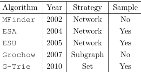
2.1 Description of subgraph count algorithms along with its release date, the type of strategy used and the possibility of a sample option . . . 8

4.1 Different networks used . . . 31

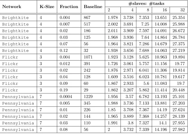
4.2 Comparison of the number of tasks computed with a different number of cores among different networks . . . 34

4.3 Comparison of the time required to reach the sweet spot computed with a different number of cores among different parameters for the Brightkite network and subgraph 4 count . . . 36

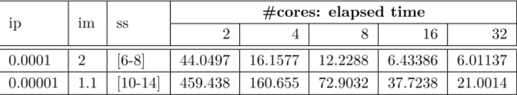
4.4 Time elapsed in order to reach the sweet spot of [10 − 15] seconds in the most time consuming network flickr with size 3 across different parameters . . . 37

(16)

(17)

List of Figures

1.1 The Dolphins Network along with its 3 5-clique subgraphs. . . 2

2.1 Motif example in a directed network. Picture taken from [25] . . . 7

2.2 ESU search tree to count all occurrences of 3 sized subgraphs in a small network. 9

2.3 G-Trie for all 4 size subgraphs . . . 10

3.1 Plot showcasing a typical fashion in which a sweet spot is reached . . . 25

4.1 Tasks completed by slaves across different singular task execution times. The results are taken from computing the census in the Brightkite network for the size 4 subgraphs with 15 minutes to run. . . 33

4.2 Sweet spot ping pong . . . 35

4.3 Labels of the different k sized subgraphs. This label is achieved by performing a DFS on the G-Trie 2.3 . . . 38

4.4 Progression of both individual and aggregated results in the Brightkite network sized 4 across different subgraph types. Every task run was done with 1e−7 probability. . . 39

4.5 Precision across different sweet spots subgraph types for the Brightkite network size 4. This results were obtained after 100 seconds of run time . . . 40

4.6 Precision across different sweet spots subgraph types for the Brightkite network size 4. This results were obtained after 300 seconds of run time. . . 41

4.7 Precision across different sweet spots subgraph types for the Brightkite network size 4. This results were obtained after 15 minutes of run time. . . 42

4.8 Average precision across different fractions of exact time. Brightkite network with 4-size subgraphs. . . 43

(18)

(19)

List of Algorithms

1 High-level methodology overview . . . 17

2 High-level Sweet spot find method . . . 18

3 Master Workflow . . . 23

4 Slave Workflow . . . 23

(20)

(21)

Acronyms

SS Sweet Spot

MS Master-Slave

IP Initial Probability

IM Initial Multiplicative Factor

MF Multiplicative Factor

MPI Message Passing Interface

CPU Central Processing Unit

GPU Graphics Processing Unit

RAM Random-access Memory

(22)

(23)

Chapter 1 Introduction

Complex networks have become more popular over the years due to their inherent ability to solve multidisciplinary problems once they are modeled accordingly. Applications of network science

methods can be found in fields such as mathematics, physics, biology or sociology [5]. With the

surge of the internet, the volume of data available on different fields is increasing exponentially making the efficient study of these complex systems the more important. The social problem

of finding the minimum distance connecting two different persons [2] and route planning in

road/transport networks [5] are only a few examples of real world applications taken from the

study of network science.

Since the applications of this area are rapidly expanding to every scientific field, different and more complex methods of analyzing the respective networks are required depending on the desired goals. Computing the average vertex degree, finding sets of closely connected components

to define them as communities [4] or discovering patterns in networks that are over represented

when comparing to an arbitrary network with similar characteristics (motifs [20]), are only a few

ways to synthesize and extract valuable information from a given network. Counting a particular set of subgraphs in a large network can thus be seen as a primitive task used by more advanced metrics in order to extract valuable information.

Even though the previous mentioned task of counting subgraphs can be seen as a primitive task, its computational complexity is not "primitive" at all. This count is bounded by the subgraph isomorphism problem, that is the problem of, given two graphs G and H, finding whether G

contains a subgraph isomorphic to H, is known to be in the NP-Complete class [15]. This

restriction makes it so that counting high order subgraphs or counting them in a large network cost too much computational time with small increases to those dimensions. To showcase how

fast this problem can scale, consider the Brightkite network presented at 4.1, counting all

subgraph types with 3 nodes took only a second to be computed and 12 million occurrences were found. If we change the subgraph size to 4, the task takes 100 seconds to complete and near 200 million subgraphs are found. Note that this experience was completed using the G-Trie exact

(24)

2 Chapter 1. Introduction

Figure 1.1: The Dolphins Network along with its 3 5-clique subgraphs.

With this exponential increase of complexity when increasing the size of the subgraphs wanted and/or the size of the queried network, different strategies have been used in order to reach those dimensions. Using parallelism is a way of taking full advantage of the available computational resources and parallel strategies are able to, in most cases, reach almost linear speedups meaning that we can divide the total time that a task would take to complete by the work units at our disposal. Another way in which this goals can be reached is by using sampling instead of having the exact count. It is possible to only search for a fraction of the subgraphs and if we were to extrapolate those results, we would get an approximate count rather than the exact one. This option is only viable if we can tolerate some error but it is really useful to get a general idea of the network’s properties in a much smaller amount of time.

The main purpose of this work is to tackle the mentioned problems and to be able to search for higher end subgraphs in larger networks. We chose to adapt a state of the art data structure

(25)

1.1. Thesis organization 3

and algorithm called G-Tries [27] so that we would use both parallelism and sampling to lower

computational times and make it possible to run more difficult tasks. Another problem we tried to tackle is the difficulty of knowing beforehand how much time a certain task in a given network would take since a seemingly lower order subgraph count in a network can be run in seconds and can take hours or days if the network were to change. In order to respond to that we present an adaptive scheme that changes and adapts its strategy to accommodate to the given network and subgraphs as good as possible with no previous information.

In this work, the count of subgraphs of a given size is done in an adaptive fashion, that means that we want to start with small and controlled tasks and successively tweak some parameters in order to adapt those so that we can create jobs that run in a desired time frame. We use a Master-Slave parallel scheme so that the Slaves can focus on doing pure computation while the Master makes sure to process each result as it arrives, crafting the next tasks using every previous result and in the end it will deliver its best guess to the subgraph counting problem. The user of our work is able to select a time limit in which he wants the results to be delivered and it is the Master’s job to make good use of that time frame. The notion of a sweet spot is present in this work and it is related to a time interval in which our ideal task should run. If we have 1 minute to run our method and set the sweet spot to 1 second, the desired goal is to start by finding a single job that takes 1 second to run, and then run it as close to 60 times as

possible. A revamped G-Trie data structure 3.2.2is used so that multiple slaves can work on it

at the same time with possibly different tasks.

1.1 Thesis organization

This work is divided into 5 chapters.

Chapter1starts of by introducing subgraph counting and gives a high level overview of its

limitations along with some ways in which we propose to tackle those problems.

Chapter 2 introduces terminology and related problems while describing some existing

approaches for subgraph counting. These approaches are divided into three categories: classical, parallel and sampling. In this chapter, we also dive into ways of representing a network when the adjacency matrix is not small enough to fit into memory.

Chapter 3 showcases our solution to the problems presented earlier while diving into its

methodologies and difficulties. We also try to justify some of the choices made along the way and present details on the different components that are part of our final project.

Chapter 4is reserved for experimental results. Here we try to show results that can back up

(26)

(27)

Chapter 2 Background and Related Work

2.1 Concepts and Terminology

• A graph G is a set of vertices V (G) along with their connections E(G). The size of a graph is usually determined by its number of vertices | V (G) |. An edge (u, v) ∈ E(G) if there is a connection from u to v.

• In a directed network, the order of the vertex on an edge is relevant since (u, v) ∈ E(G) 6=⇒

(v, u) ∈ E(G). In non directed graphs however, this is not true since all of the edges in this type of network are bidirectional.

• A graph is typically represented by a adjacency matrix Adj which is a | V (G) | × | V (G) | boolean matrix. Adj[u][v] = 1 if (u, v) ∈ E(g).

• A graph H is said to be a subgraph of G if E(H) ∈ E(G) and V (H) ∈ V (G). That

subgraph is said to be induced if ∀u,v ∈ V (H), (u, v) ∈ E(H) ⇐⇒ (u, v) ∈ E(G). A

occurrence of H in G happens if there is a set of vertex that induce H. We define multiple occurrences as different set of vertex that induce a particular subgraph H.

• A vertex u neighborhood N (u) is the set of vertex v so that (u, v) ∈ E(G). A vertex u exclusive neighborhood respective to a vertex set S is composed by v so that v ∈

Vexc(u, S) ⇐⇒ v ∈ N (u), v /∈ N (w)∀w ∈ S.

• A k-sized graph/subgraph is a network with size (| V (G) |) k. A k-clique is a graph of size

k in which every vertex is connected to every other ∀u,v(u, v) ∈ E(G).

• The degree of a vertex v is the number of different vertex u to which it is connected. In a directed network we can differentiate between indegree and outdegree depending if we are considering u, (u, v) ∈ E(G) or u, (v, u) ∈ E(G). In non directed networks, there is no need to distinguish these measurements since they are always the same.

(28)

6 Chapter 2. Background and Related Work one edge connecting two vertex. We also assume a label of the vertex so that a size-k graph will have nodes labeled 1..k.

• A permutation is a unique ordered way in which we can arrange a set of elements. Two permutations are distinct if at least one of the elements is in a different position in the set. For a set of k elements, there are k! unique permutations.

• We define two graphs G1 and G2 as isomorphic if they have the same size and there is a

permutation p of G₂, Gp₂ so that ∀u,v, (u, v) ∈ E(G1) =⇒ (u, v) ∈ E(Gp2)

• An automorphism is a particular type of isomorphism that maps vertices from G so that the resulting graph is isomorphic to G.

2.1.1 Subgraph Count

Given a network G and a size k, the subgraph counting problem lies on counting all occurrences of each different size k subgraph on the original network. A occurrence of a particular subgraph is defined as a distinct induced group of vertex.

2.1.2 Network Motifs

Even though this work is not intended to be focused solely on motif discovery, this task is still one of the main problems we are trying to tackle.

Motifs were introduced by Milo et al. [20] as patterns whose frequency is much higher than

the one found in similar random networks. This task is not to be confused with Frequent Graph mining since a subgraph with high frequency in the original network is not necessarily a motif. Most of the approaches to the motif discovery problem can be divided in four main tasks:

• Finding and counting all of the k-sized subgraphs occurrences in the original network • Generate a set of similar random networks.

• Count the frequency of each of the original subgraphs in the random networks • Compute the significance for each subgraph type

When considering a network G, we define a similar random network as a graph with the same size as k with the same number of edges in which the node degrees are preserved. The significance that is calculated at the end of the motif find procedure is usually the Z-score which is a measure that takes into consideration the number of standard deviations from a score to the mean of all the results.

(29)

2.2. Subgraph Count Algorithms 7

Figure 2.1: Motif example in a directed network. Picture taken from [25]

In picture 2.1 we can see an example of a motif in a subgraph along with the respective

similar random networks. The Feed Forward Loop presented only has one or zero occurrences on the generated networks while it can be found multiple times in the original network. We can see that the random networks preserve both indegree and outdegree for every vertex.

2.2 Subgraph Count Algorithms

We can classify the algorithms for subgraph counting in two major groups. The network-centric approach that fully extracts the count of all subgraphs with the desired size and then matches each of those with the matching isomorphic type. Subgraph-centric options start with a specific isomorphism class and count its occurrences on the network. A set-centric approach can also be considered as an intermediate approach between the two major ones if we are neither searching all of the subgraphs, neither only one of them but rather a specific set. One can, for instance, only be interested in 4-cliques and "squares" while doing a subgraph count of size 4 on a certain Network.

(30)

8 Chapter 2. Background and Related Work

Algorithm Year Strategy Sample

MFinder 2002 Network No

ESA 2004 Network Yes

ESU 2005 Network Yes

Grochow 2007 Subgraph No

G-Trie 2010 Set Yes

Table 2.1: Description of subgraph count algorithms along with its release date, the type of strategy used and the possibility of a sample option

2.2.1 MFinder

Milo’s algorithm for counting the number of occurrences of all the k-sized subgraphs [20] was the

first attempt at solving the problem and had some flaws. It exhaustively found all the subgraphs with the desired size and stored them in a table. After each occurrence find, the algorithm would check for a isomorphism match of the respective vertices in the table and would only store it if that isomorphism was not found, meaning that we are exploring a new occurrence. For each subgraph to be found, every permutation of its nodes would be reached, that sums to k! occurrences instead of only one along with the need to traverse the search tree that many times.

2.2.2 ESU

Wernicke [33] tackled a large portion of the problems laying in the available motif finding strategies.

He not only proposed a faster algorithm for the enumeration of all the size-k subgraphs on the original network but also presented an alternative for the random network generation.

At any stage of this algorithm we have a set of vertex and choosing one by one we try to expand them. Choosing a vertex, we expand them to a set with vertex with higher label and who are only neighbours with the chosen vector across the partial subgraph created so far. If we have two vertex a and b in our partial subgraph and we are expanding a, the expanding set is composed by vertices with label higher than a which are not neighbours with b. The labeling restriction helps with symmetry breaking since we only extend a vertex from another and not the other way around and it is this property that makes sure that each subgraph is not only found but is found exactly once. After this step the algorithm will try to recursively extend a vertex at a time and stop if either the desired subgraph size is reached or no vertex can be extended under the two previous stated conditions. This method provides a computing tree and

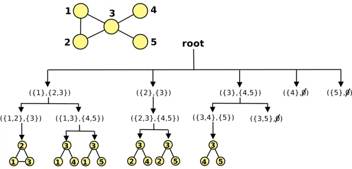
bellow the root are the sets of each vertex coupled with its extension set. Figure 2.2showcases

(31)

2.2. Subgraph Count Algorithms 9

Figure 2.2: ESU search tree to count all occurrences of 3 sized subgraphs in a small network.

2.2.3 Symmetry breaking conditions

Since the first algorithms for subgraph count and consequent motif find had size limitations,

Grochow et al. [7] presented a new idea based on a singular query subgraph, a subgraph-centric

approach. A complete census would be computed in this fashion by using a graph enumeration

tool such as McKay’s geng and directg [18].

In order to address the problem of finding the same subgraph more than once due to

isomorphisms, Grochow et al. [7] purposed a novel algorithm to limit those tests using symmetry

breaking conditions. The isomorphism tests to see what type of subgraph was found were also improved in this method.

Successive calls to find isomorphisms for the wanted subgraph onto the original network are made in a backtracking search. This phase tries to select nodes with many neighbors which are already mapped and whose degree is higher. A single call to this method extends the partial match by a single node. That new node has to be connected to the remaining nodes according to the wanted subgraph type isomorphism we are trying to find. These tests at early stages made sure that we are able abort computations in earlier stages, which was not possible in previous methods. A single subgraph type can be mapped in a network in different ways. For instance, a triangle a, b, c can me mapped into the 3-clique subgraph type in 6 different ways. In order to avoid this repetition due to symmetries, some restrictions are computed and those symmetry breaking conditions ensure that there is a unique match of a group of vertex to a subgraph. Simply ignoring automorphisms and count the same occurrence more than once (in a different

(32)

10 Chapter 2. Background and Related Work Using a labelling for the nodes, conditions of the form L(n) < L(m) for two nodes, we make sure that any ambiguity due to them being in the same equivalence class is settled. This conditions are enforced until all the nodes are fixed.

2.2.4 G-Tries

The G-Tries are a novel data structure proposed by Ribeiro and Silva [27] with the purpose of

improving the available algorithms and speeding up the process of subgraph counting. This data structure is the main pillar of this work.

It takes advantage of common substructure between graphs, like a prefix tree would, being able to compress space usage. G-Tries also uses symmetry breaking conditions in order to make sure we find each subgraph only once and not waste redundant computation time. Besides being fast, G-Tries are also generalist, being able to be used in most graph types such as directed, weighted or colored. It also allows for a query on a particular set of subgraphs, from a single one to the all of the k-sized subgraphs.

In a string trie, every node represents a single letter, in a G-Trie the node represents a vertex in the graph. Having two nodes with the same parent in the G-Trie means that you will have the same graph if you remove that node.

Figure 2.3: G-Trie for all 4 size subgraphs

The process of creating a G-Trie is also similar to creating a trie. We start with an empty tree and insert the desired subgraphs in an iterative fashion. We traverse the tree until we find a node in which none of the children matches our subgraph and in this case all of the remaining nodes will have to be created. The problem with this method is knowing in which order should we consider the subgraph vertex since a different order could lead to a different G-Trie. A

(33)

2.2. Subgraph Count Algorithms 11 canonical form has to be used in order to shape the G-Trie in a deterministic fashion and there is a custom canonical form designed in order to increase the memory compression by identifying and taking advantage of common substructure. That canonical form is illustrated at the figure

2.3and other less efficient canonical forms are shown to be less compressed [25].

G-Triesare also advantageous to use for space complexity reasons. This tree organization

scheme occupies less memory and scales better for larger sizes. Increasing the amount of common substructures leads to a lower space usage that what we would have if we were to simply use the

adjacency matrix for each of the queried subgraph [28].

After having the G-Trie ready, we can start counting the respective subgraphs on a given network. Here we will be partially matching the graph trough the G-Trie until we either get to a final node or to a dead end. At a given node, we compute the set of remaining nodes that can still be added to the partial graph and choose one of them, check if it matches the current node, and if so, then recursively try to match the rest of the G-Trie and in the end, change the chosen vertex. We check if a vertex matches the a G-Trie node if it has the same connections to the previous vertices and if so we either continue the algorithm or stop if we reach a leaf. The former means that we found a specific subgraph from the desired set and in that case we can increment its count.

Some previous methods of counting did not include any automorphism tests and we would have to count the same subgraph multiple times (n!) and divide the final count by that number similarly

to what was done in [20]. G-Tries are also equipped with symmetry breaking conditions that

remove the need to compute the same subgraph over and over. This idea was introduced by [7]

and was adapted to the G-Tries. In each G-Trie node we have a list of conditions regarding the label of the nodes. For instance l(a) < l(b), l(d) < l(c) means that both the label of a has to be lower than the label of b and the same with d and c. The structure of the conditions is also ready to remove redundant conditions in order to decrease the time required to test them.

2.2.5 Other sequential algorithms

We chose to focus our attention on some classical algorithms which introduced fundamental steps that allowed for the former ones to be conceived. There are however many more ways available to tackle the subgraph count problem. There are some methods which are better for some cases and worse for others but there are also some fundamentally different strategies of tackling this problem.

FaSE[21] uses a customized G-Trie that is build during the algorithm execution on the fly,

instead of building it before even starting any kind of computation. FaSE creates intermediate topological classes postponing temporally the isomorphism tests. This algorithm is divided into two steps, the enumeration, which is similar to other explored algorithms, and encapsulation,

(34)

12 Chapter 2. Background and Related Work tests and presents a quaternary tree data structure at its core. That quaternary tree is similar to the G-Trie and computes partial classifications for enumerated subgraphs.

There are some analytic algorithms that attempt to bypass the step of counting all occurrences by taking advantage of combinatorial characteristics of the networks. Due to the usage of those properties, this methods are often limited to particular network types and subgraph sizes.

acc-Motif[19] is an analytical algorithm to count subgraphs of size k + 2 in a rapid fashion

based on the count of induced subgraphs with size k. The main drawback of this method its inability to easily be adapted to larger sizes. This algorithm is conceived using combinatorial techniques along with a frequency histogram.

ESCAPE [23] provides an algorithmic framework used to compute the exact count for the

5-sized subgraphs. This analytical method uses pattern division and exploits degree orientations related to the graph in order to achieve high performance counts. In this method, only four subgraphs are required to be enumerated so that the final 5-size counts are outputted and this result is proven as part of the work. This method avoids the enumeration along with its inherent combinatorial complexity.

2.3 Parallel Approaches

In order to fully take advantage of a computer or a cluster of them, parallelism can be explored and in ideal scenarios, close to linear speedup can be achieved. This means that a task that

took x units of time to compute would ideally take _nx units of time when n refers to the number

of available cores. There is work in both distributed and shared memory related to subgraph counting. In distributed schemes, the programmer can count on multiple independent work units, each with their own memory. In shared programming, all the different work units share the same memory. Generally speaking, when using shared memory, the cost of communication is lowered but its harder to account for race conditions between different work units. There can also be hybrid approaches where there are multiple units, each with its own shared memory.

2.3.1 Parallel G-Trie for Distributed Architectures

The G-Trie data structure and census computation algorithm produces a search tree in which every call to a procedure is independent from one another. Noticing that and with

the goal of accelerating the subgraph count problem, Ribeiro et al [26] adapted the former

work to a distributed parallel scheme using the message passing interface (MPI) implementation

OpenMPI [6].

In order to start a parallel algorithm it is useful to be able to divide the wanted work in logical pieces usually called work-units. In this particular algorithm every recursive call to the matching function, which tries to match a group of vertex with a new one in order to later associate it

(35)

2.3. Parallel Approaches 13 with a size-k subgraph, is considered as a work-unit and the main problem is to divide those work-units among all processors. Even though the algorithm is traversing a computation tree, the work load is not balanced among the nodes making it hard to statically divide the work without ending up with some workers doing substantially less work than others. The dynamic fashion in which this algorithm divides its work is a receiver-initiated scheme. Each processor chooses part of the available work and computes it while periodically checking for messages from the other processes. That check phase has the goal of seeing if any other processing is requesting more work and if that is so, the recursive calls are stopped and the computation state stored, the remaining work is divided and half of it is send to the message sender. Due to how imbalanced the associated tree can be, the work is divided in a round robin fashion and the processor who is giving part of its computation array keeps the currently explored nodes. This algorithms is tailored so that there is a threshold related to remaining work so that a unit with little computation to do doesn’t spend time splitting it. This case would end up in the original processor simply asking a different thread for work division. In a final phase, each subgraph type count has to be aggregated in order to get the final count and this is accomplished by using the native reducing procedures of the used interface.

2.3.2 Parallel G-Trie for Shared Memory

When performing a census on a G-Trie, we are essentially traversing different tree branches

that are independent from one another. Noticing that, Aparício et al. [1] adapted the previous

G-Trie census algorithm to a Multicore Architecture in order to parellelize a single census.

Simply dividing the branches in a static fashion was not good enough due to how imbalanced different k-sized subgraph counts can be for a single network. In this work each core is assigned a thread and the vertex are divided among them. Each thread will now compute the census as it would in a sequential fashion until it has no more work to do. When a thread finishes its work, it asks for another random thread to split some of the remaining work. Since different threads may find the same subgraph type with different sets of vertex, each thread would have a private count of each subgraph type and in the end, the global frequencies would be attained by summing every thread counts.

2.3.3 Parallel ESU for discovery of motifs

In order to speed up motif discovery, Ribeiro et al [26] provided a method of performing all

of the required steps for motif discovery in parallel, namely the census and both the random

network creation and subgraph count. Since in the ESU algorithm [33] the calls to extend a

partial subgraph are independent for each other, they can be computed in parallel with no synchronization required. After being able to divide the bigger picture into smaller tasks, two

(36)

14 Chapter 2. Background and Related Work strategy has all of the workers responsible for both computing and communicating to divide work. Before starting the main computations, a pre-processing phase takes place. The required jobs are divided among workers either by sending all of it to a single unit, expecting that other workers will steal some of the work, or by statically dividing the jobs among work units in a round-robin manner. In the Master-Slave strategy, the master is continuously receiving messages from its slaves. If it gets a message requesting work it can either send unprocessed work or add that slave to a queue of workers waiting for jobs. If it receives a message with more work, it can send it directly to an idle worker or add it to the work queue. This process ends if all of the workers are idle. In the Distributed option, the work division is made by all of the cores which are all equal in this strategy. Each worker keeps computing its work until it has no more computation to do. In that case it asks another random worker for part of its remaining computations and continues. The choice of another core to steal work from is random due to how imbalanced and unpredictable the tree branches can be. If a request for more work is made to another core waiting for work, another random choice is made and if that process keeps repeating among all the workers, we can conclude that there is no more computation to be made and the count process is finished. The final step of this process is to gather the results from each worker to a chosen one, responsible for the significance calculation. This is done by fixing an order in a vector. A position in that vector denotes both the network and the count of a particular subgraph type. The workers are then organized in a binary tree fashion with the selected worker at the top. After aggregating all of the results, that root worker sequentially computes the significances and later return the found motifs.

2.3.4 More parallel approaches

Even though we dived into the parallel options which were the most related to our work, there is more to parallelism in graph analysis.

Ahmad and Ribeiro [29] tackled the subgraph count problem in a parallel fashion using

MapReduce. MapReduce is a programming model aimed to process large amount of data and it is inspirited by the map and reduce operations available in the functional programming paradigm. The presented method works on top of G-Tries, it is able to dynamically share work among the available work units and it is directed to cluster computing in the cloud.

Lin et al. [14] takes advantage of parallelism in a different manner. Their work focus is on

Graphical Processing Units (GPU) and its inherent parallel aspects due to its high number of processing units in order to simultaneously perform different subtasks related to motif discovery. The CUDA framework is used in this work in a very detailed fashion and its respective results are not only competitive to the existing CPU approaches timewise but also cost effective when the prices of these different processing units are considered.

An hybrid option between CPU and GPU usage is presented by RA Rossi and R Zhou [30].

By simultaneously taking advantage of both these types of processing units along with its different strengths, a fast algorithm for extracting information from a network regarding induced

(37)

2.4. Subgraph sampling 15 k subgraphs is presented. The results obtained by this method fully use the available processing resources and are not only fast but also cost and energy efficient.

2.4 Subgraph sampling

With the goal of being able to aim for higher order subgraphs or to be able to find them in larger networks, there has been work dedicated to trade accuracy for speed in the form of sampling. Most of the sequential algorithms presented in the respective section can be adapted to search only a given fraction of the subgraphs rather than the whole set. This is typically done by moving in the computing tree only with a certain probability when there is a tree like structure. The way of distributing the fraction across levels is not obvious and can be achieved using different strategies.

2.4.1 Kashtan

Kashtan et al. [9] introduced the concept of sampling in motif discovery. After the initial census

on the original network, this method would sample each of the random networks instead of exhaustively counting each subgraph occurrence by picking a random edge from the graph and then iteratively choosing a random neighbour edge until the desired size is reached. The sampled subgraph is then composed by all of the nodes found along with all of the edges between them (not only the expanded ones in the sampling process).

2.4.2 Rand-ESU

The ESU algorithm was presented along with a sampling version [33], making it possible to

effectively trade speed for result accuracy. In order to sample the ESU-tree a given probability is divided across all the levels except the last one so that the product of each partial probability on

the levels was the original probability. If there are k levels, assigning a probability of pk1 on each

level would assure the previous condition. Wernicke noticed that a cut on a branch closer to the tree would highly influence the rest of the run compared to a cut closer to the leafs.

2.5 Alternative graph representations

We are trying to explore the subgraph problem on large and complex network in which the size of the graph has to be addressed. Since a typical representation of a graph as an adjacency matrix

(38)

16 Chapter 2. Background and Related Work a graph so that it would be small enough to fit in memory. Of course that we are giving up the O(1) cost of the operation to see if there is a connection between two nodes and so the execution times are expected to be higher when using this options. Graph representations such as a sorted list so that binary search can be used and hash table based on both nodes and edge are explored in depth. In the end Paredes uses a hybrid approach, combining several methods, and reaches performances only two times slower than the adjacency matrix.

(39)

Chapter 3 Methodology

In order to solve the subgaph counting problem, we purpose a high-level adaptive strategy whose goal is to be able to deliver the best guess possible relative to the frequency of each subgraph type in a given time frame. Afterwards we concretize this idea using the G-Trie data structure with its sample version as the base and modify in order to make parallelism possible. Sampling is used since we are trying to search complex networks in which the exact count would take too much time and the parallel component will make sure that we can do more computation in that selected time frame, compared to a sequential approach.

This work is directed so that it is possible to shape the algorithm according to the queried network’s characteristics, the subgraph size and the available time. We want to find a task that is able to run in a desired time frame and once task is crafted, we can complete it over and over until the available time is over. The ideal sweet spot is a time frame in which we want our computation to fit. The goal is to tune some parameters, namely the fraction associated with sampling, so that we can rapidly craft a task that would lead to that sweet spot.

3.1 Overview

Algorithm 1 High-level methodology overview

1: idealT ask ← f indSweetSpotT ask()

2: while not timeIsOver() do

3: idealT ask

4: end while

5: aggregateResults()

(40)

18 Chapter 3. Methodology

Algorithm 2 High-level Sweet spot find method

1: task ← initialT ask

2: while elapsedT askT ime /∈ idealInterval do

3: task ← ref ineT ask()

4: end while

5: return task

A simplified version of our methodology is described at algorithm3.1. We start by finding

our ideal task (line 1) and then repeat it until the time period given by the user runs out (lines 2 - 3). After the time runs out, we gather the results and output them (lines 5 - 6). Note that the definition of the ideal task can be provided by the user or by some automatic parameters

suggested at sections 3.4.1 and3.4.2 and besides that, the aggregation phase can be updated as

new results arrive.

The general process of finding the ideal task, given a time frame, is described in algorithm

2. We start by computing some initial task (line 1) and proceed by refining it until it fits the

desired time frame (lines 2 - 4). After the "perfect" task is crafted, the process stops, and its characteristics are returned (line 5).

We want to make sure that we can run this method in networks in which the time required to do a complete census would be overwhelming. With that in mind we chose to start with a small,

conservative sampling fraction of the desired count such as 10−10, measure the time associated

with that fraction and change it until it fits our time goal for a task. Along with that initial probability initialP rob, we also provide a multiplicative factor initialM ultF actor to determine the next probability to be tried. A single task in this algorithm can still take too much time to run and in this case, we decided to lower the probability to the last "feasible" task, change the multiplicative factor and continue from that point.

The Sampled G-Trie presented by Ribeiro and Silva [26] is the algorithm used to do the

successive sampled census required. More information about what fraction is used and its

distribution among the different G-Trie nodes will be detailed at section 3.2.4.1. Parallelism is

included in this methodology so that we can achieve the desired sweet spot faster, by sending different workers to compute different tasks. Also, parallelism will make sure that we can have more repetitions of the final, ideal job as more cores are added. In order to enable parallelism, the original G-Trie was modified so that it would support multiple units performing computations

(41)

3.2. Parallel methodology 19

3.2 Parallel methodology

3.2.1 Parallel opportunities in the subgraph counting problem

Parallelism was considered and applied to this work with the main goal of making it possible to run potential different jobs independently from one another at the same time. Each job can be assigned to a single work unit with its own sampling probability distribution. Parallelism could

also be applied to a make a single run faster [1] but it is not the main focus of this work.

3.2.2 Revamped G-Trie

In order to be able to run our parallel algorithm, the G-Trie structure had to go trough some changes. It was possible to have a copy of the G-Trie in each work unit and simply run the wanted tasks in that particular copy but that would possibly take too much space. With the goal of lowering that space usage, and given the fact that we would be mostly doing memory reads until the count increment stage after a match between the original network and a particular subgraph type is achieved, we adapted the base structure so that it was possible to run several census at the same time in a parallel fashion.

The base data structure was changed in a way that each work unit would have its own copy of each non shared variables. We coupled those variables in a structure and chose to use an array of those structures rather than single arrays for each variable due to cache efficiency problems. When a variable was requested, instead of loading into memory every work unit’s variable of the same type, we would be loading all of the non shared variables related to that thread. This arrangement of the variables only proved to be the right choice after also making sure that the structure combining all of those variables would take exactly a cache line (in a hypothetical case, any number of fully filled cache lines would work) because if that was not the case, we could have a thread’s respective structure being divided among different cache lines and that would result in constant cache misses. This was achieved by adding a padding dummy variable to fill the remaining of the structure.

This padding adjustment decreased the number of cache misses and was proven instrumental in order to achieve linear scaling on the parallel G-Trie.

We also added the possibility of searching a custom set of subgraphs instead of the whole set. This was done by adding a boolean label to the G-Trie nodes that would tell us if that node

(42)

3.2.3 Master-Slave Architecture

A master/slave architecture is a programming model where one or more components, the masters, have control over the remaining components, the slaves. The master, in this strategy, is often the one who decides what jobs each slave is doing and is the entity responsible for scheduling and dividing work among the slaves as well as aggregating their respective results. The slaves are mostly responsible for requesting a task, doing its associated computation and delivering the results back to the master.

Usually we can separate some different stages in this strategies, the work division phase, the computation phase and the result aggregation stage. The work division phase can be either static or dynamic. In static approaches, the work division can be made at the beginning, with the associated disadvantage that a static partition may provide unbalanced work among slaves, potentially forcing the slaves to be idle after their respective share of the work is completed, wasting computational resources. Dynamic approaches tend to have higher overheads due to more frequent communication across work units but will likely provide a more balanced work division. Dynamic work divisions can be made either by the master, who will create new tasks as soon as slaves computations are ending, or by the slaves who can steal part of the work from other workers when they finish their initial share.

The Master-Slave paradigm was the one chosen to make use the of multiple cores available. This strategy was used since we found it useful to have a central entity managing all of the jobs with the possibility to interrupt some and change parameters of the future ones with no need of synchronization among the remaining working cores. This strategy was chosen over others specially due to the adaptive component of this work. Since we start with little information, it is useful to have a central master trying to queue different magnitude tasks and adjust them to the desired time frame.

3.2.4 Adapting Master-Slave to the subgraph counting problem

The main idea of this architecture is to have a queue of jobs generated by the master and a queue of results to hold the calculations performed by the slaves. The job queue will be updated as results of previous tasks come to the master in an adaptive fashion. For instance if we notice that a job with a set of parameters took too much time, the master can simply stop all of the workers who are doing similar things and they would poll the queue for new tasks to perform. In this method, the slaves simply grab tasks from the queue, compute the census associated with the task and send the results to a results queue. The master will be keeping track of both completed tasks and queued ones and will manage the slaves work while processing completed computations and crafting better tasks for future stages.

(43)

3.2.4.1 Work units and Job Queue

We define a work unit as the essential information that a certain worker should have in order to complete a particular task crafted by the master. A work unit, in this architecture, is defined by a scheme, a fraction and the labels regarding the subgraphs that we want to count. The fraction in this work unit is the part of the graph that we want to sample. There are different ways in which we can divide the same fraction across the G-Trie levels and the available schemes are

the ones proposed by Ribeiro and Silva [26] and can be divided in three when fixing the subgraph

size k and the fraction f .

• low: P₀= k−1√_{f , ..., P} k−3 = k−1 √ f , Pk−2= k−1 √ f , Pk−1= 1 • medium: P0= 1, ..., Pk−4= 1, Pk−3 = √ f , Pk−2 = √ f , Pk−1 = 1 • high: P0 = 1, ..., Pk−3 = 1, Pk−2= f, Pk−1 = 1

The initial motivation for having these different ways to divide the probabilities across different levels was to have more flexibility regarding the distribution of that particular fraction among the G-Tries nodes. For a fixed fraction, we could chose the low scheme if we wanted faster and less accurate results, high scheme if we had enough time and wanted a count as precise as possible or medium as an in between option. At later stages of development, the option to switch schemes was particularly important since we found it impossible to reach some desired time frames with the high scheme since it was bounded by the exact computations associated with the previous size problem (k − 1). This happens due to the fact that fraction of each level but the last is 1. In those cases we can switch the scheme to low and craft tasks with the desired time frame while running the same adaptive ideas.

The job queue holds this sort of structures and it is filled by the master who tries to keep it

with 2 × n_cores at every computation stage. The same queue is polled by the slaves at any stage

in which they aren’t doing any computation. More details on the this queue implementations

can be read at the section 3.2.6.1.

3.2.4.2 Aggregating partial results

After doing a specific task, each worker will communicate the results found to the master. We keep track of the sampled count of each subgraph enabled, the time elapsed in the respective

(44)

3.2.4.3 Acting according to ongoing computation state

Even though both previous mentioned queues would be enough for this strategy to work, we would not be able to check neither the running jobs for each slaves neither would we be able to check if a particular task was taking too much time. In order to address this problem, third structure was used in this strategy, a vector of running jobs with a entry for each slave. The purpose of this structure was to make it possible to the master to scan what every slave was doing giving it the ability to interrupt some of the tasks. This third queue would hold, for each running task, the id of the thread that was processing it, the time associated with the start of the

task along with the respective work unit with the information described above at section 3.2.4.1.

3.2.5 Finishing criteria

With the purpose of allowing for multiple goals, we set a few ways to stop the whole sampled

subgraph count process. We can provide running time and/or a convergence metric and

convergence value. If the master notices that it has been running for longer than the time set by the user, it will stop the slaves and output the results. The same will happen if the results converge to a given value given a certain metric. If we finish a job with probability 1 over all of the labels, the program will also end since we just did a complete census and the results will be the ones got at that final iteration.

3.2.6 Master-Slave work flow

Our whole process is always controlled by the master and it is the master that is called at the

beginning of this strategy. Algorithm 3describes this component’s work flow.

After being initially called, the master starts by doing some setup operations (line 1). This setup includes launching the slaves threads, filling the job queue with some initial tasks, loading the network and the G-Trie among other beginning tasks. It will then start its main body consisting of generating tasks and aggregating upcoming finished computations (lines 2-9) until the given time is over. The slaves are checked periodically to see if they are doing meaningless computation such as tasks running for longer the desired ideal frame and tasks whose characteristics are already proven to result in higher executions than desired (line 3). If the job queue is getting empty, the master fills it with new tasks based on the previous results attained (line 4). The master will check for new results and process them if so. This result process stage will partially aggregate the latest result and update some variables which are instrumental in determining future tasks (lines 5-7). At the end of the available time, the master does some cleanup operations such as shutting down the slaves and then it can simply output our results as the guess for the subgraph count problem since the master is updating results as they come by (lines 10-11).

(45)

Algorithm 3 Master Workflow

1: setup()

2: while not f inished() do

3: checkSlaves() 4: addT asks() 5: if newResults() then 6: res ← resQueue.pop() 7: processResults(res) 8: end if 9: end while 10: cleanup() 11: outputResults()

The slaves workflow is simpler than the masters but very important nonetheless. It can be

described at algorithm4.

The slaves are always on a loop computing whatever results required (lines 1-7). If they have work to do they start by getting a work unit from its queue, run the associated task and output the results to the result queue (lines 2-5).

Algorithm 4 Slave Workflow

1: while true do

2: if workT oP rocess() then

3: workU nit ← workQueue.pop()

4: res ← runCensus(scheme, f raction, labels)

5: resQueue.push(res)

6: end if 7: end while

3.2.6.1 Parallel synchronization, cancel methods and implementation details

One of the goals of using this architecture was to remove part of the inherent synchronization that would need to happen if there was no master managing all of the slaves.

There are, however, a few sections that are protected with locks. Namely the working and the results queue. The master must be sure that no slave is popping the tasks queue when adding new tasks and when the master is getting results from the respective queue, no other unit can be accessing it. We decided to implement our version of a parallel queue, coupling each queue with its respective lock mechanism, so that it would have to be acquired in order to do the regular queue operations such as pushing, popping and emptiness test.

(46)

24 Chapter 3. Methodology the deferred types. When at the deferred state, a thread can only be canceled at a cancellation point. This is useful if we have a series of operations that need to be considered atomic. The asynchronous type allows a thread to me canceled at will.

We chose to set cancellation points both at the beginning and the end of each iteration and chose to set the census as asynchronous so that it can be interrupted at any time. If, for instance, a cancel request is made right after a finished census, the cancellation type is already deferred and the slave will only cancel after sending its respective results. It was this deferred option that made sure that a thread wouldn’t be cancelled, for instance, after acquiring a particular lock, which could cause a deadlock after being cancelled.

The slaves are periodically checked by the master and can be set to be canceled if they are taking too much time (this threshold is set to be 2 × sweetSpotF inish by default) or if they are doing a task that is known to run outside the sweet spot. This final situation can happen if the master notices that a certain task is taking too much time and all of the tasks with a fraction above that one are to be cancelled. The slaves are also canceled if a finish state is reached.

3.3 Adaptive Methodology

The adaptive fashion in which we reach our ideal tasks is at the core of this work. In one hand, we want to reach that sweet spot quickly but on the other, we don’t want to start many tasks that will have to be canceled due to their excessive duration. Assuming that we have no idea of the time that a certain sample with a given fraction will take to compute, we have to be conservative with our initial probability so that we have a baseline which can be increased afterwards. We don’t want to discard valuable computational time just because a tasks takes a bit more time than our ideal task duration. We added a threshold over the desired time limit so that we can both use those results and we can use that elapsed time as a upper bound for our computations.

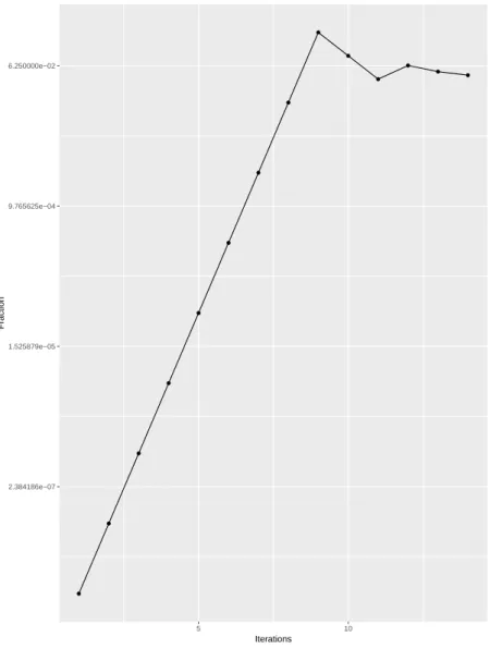
3.3.1 Sweet Spot

The idea of a sweet spot is a time frame in which a single task should compute for the best approximation of the subgraph count problem. Ideally, when a sweet spot is set, the goal is to run the corresponding task totalT ime/sweetT ime times during the available time period. Even though this concept is a parameter of our program, we present a few methods of logically defining a sweet spot.

One may think that the ideal task should be associated with a low time frame task so that it can be repeated over and over until the time given by the user for the subgraph count problem is over. This approach has the apparent advantage of being able to fit several tasks in the given elapsed time with the motivation that more tasks should provide a better guess for this problem. The problem is that, despite the high number of runs, we are always running them with a small probability and that factor can have a negative impact in our final approximation.

(47)

3.3. Adaptive Methodology 25 2.384186e−07 1.525879e−05 9.765625e−04 6.250000e−02 5 10 Iterations Fr action

Figure 3.1: Plot showcasing a typical fashion in which a sweet spot is reached. We can observe that the fraction increases at the same multiplicative rate until its associated task takes more time than expected and from that point it lowers the multiplicative factor and continues this method until the sweet spot is reached.

We can think that the ideal sweet spot should be related to a task which maxes its elapsed time. The motivation to this option is that running a census with a higher probability should give us a better estimate but its drawbacks are the lower sample size along with the tighter time restrictions since we can’t be sure of the elapsed time of a task before hand, making it hard to guess the associated probability and thus making it possible that our "ideal task" will not even

(48)

3.3.2 Reaching our ideal task

Regardless of the strategy used among the ones referred above, we need to have an algorithm that is able to craft a task that will fit in the given sweet spot restrictions. We present algorithm

5 that proves to reach sweet spots in a rapid fashion. This algorithm has two main parameters:

The initial probability and the initial multiplicative factor (lines 1 - 2). The initial probability should be conservative so that we have a lower bound task as soon as possible. Afterwards, we want to tweak the tasks characteristics so that we reach our desired job (lines 4 - 13). If we notice that a task’s elapsed time is below our time interval, we can simply create a new task with a new increased probability and reach that probability by multiplying the previous one by the respective multiplicative factor (lines 5 -6). It is also possible that after multiplying a completed task’s fraction by the associated multiplicative factor, we face a new tasks whose time frame is above our sweet spot. In that case we should proceed by returning back to the previous task’s fraction, lower the multiplicative factor, get a new fraction and continue searching for the ideal task (lines 7 - 10). If we find that a certain task fits the given time frame, that task will be the ideal one and the sweet spot finding phase can be considered over (12 -14).

Algorithm 5 High-level sweet spot reaching algorithm

1: p ← initialP rob

2: f ← initialM ultF actor

3: sweetReached ← false

4: while not sweetReached do 5: if taskT ime < sweetSpot then

6: p ← p × f

7: else if taskT ime > sweetSpot then

8: p ← _fp 9: f ← f₂ 10: p ← p × f 11: else 12: sweetReached ← true 13: end if 14: end while

3.4 Approximating the counting

Due to our method’s property of receiving several results for potential different tasks, we decided that a simple average of each count ,with its respective extrapolation ,would not suffice.

A weighted mean was the metric used since it can emphasize experiences with higher sampled fractions, which should lead to more precise counts. With a set of n extrapolate results res and associated sample fractions f rac, if we were to fix a subgraph, its estimate is given by the formulae below.

(49)

3.4. Approximating the counting 27

wAvg =

Pn

i=0resi× f raci

Pn

i=0f raci

We are interested on following the distribution of the results over the time so that we can potentially stop computations when we notice that recent results are not changing our global estimate by much. Calculating the result dispersion can be achieved by using variance and its standardized version, coefficient of variance. Since we always want to give more weight to tasks made with higher sampling portions, we will present weighted versions of these measures.

wV ar =

Pn

i=0f raci× (resi− wAvg)2

Pn i=0f raci wCoef f V ar = wStdDev wAvg = √ wV ar wAvg

Since our method is able to run tasks with execution times as little as seconds for several hours, it can be dangerous to store all the results at all times and the calculation of this metrics would take more time as more results got processed. In order to solve this problem, we adapted these formulae so that only the last run, along with a few fixed numbered variables were needed. Those new variables that are updated as a new result comes by are the number of tasks completed n,

the sum of the fractions usedPn

i=0f raci, the sum of squared weighted resultsPni=0f raci× res2i

and the sum of the weighted results Pn

i=0(f raci× resi).

The new weighted average can be simply computed with the following.

wAvgnew =

(wAvgold×Pn−1n=0f raci) + resn× f racn

Pn

n=0f raci

After updating the remaining variables, we can get the new weighted variance along with weighted coefficient of variance.

wV ar =

Pn

i=0f raci× (resi− wAvg)2

Pn

i=0f raci

=

P

f raci× (res2i − 2 × resi× wAvg + wAvg2)

Pn n=0f raci = P f rac × res2_{+ 2 ×}P f rac ∗ wAvg +P wAvg2

(50)

3.4.1 0 probability run and new ideas

The high scheme mentioned earlier at section3.2.4.1 is the starting scheme used in our runs.

There is a chance that , for a set of network and subgraph size k, the defined sweet spot couldn’t be achieved despite the fraction sampled. This weird phenomena is explained by the definition of the high scheme. The probabilities in this idea are scattered among the G-Trie nodes so that only the k − 1 level represents that fraction. This means that the count for that k is bounded by the exact count of k − 1 in this scheme.

This realization made us adapt our algorithm so that it would always start of by computing the lower bounded 0 probability in the high scheme (with the only goal of seeking a lower bound for the default scheme) run and if the respective elapsed time was over the defined by the user, we could switch the method to low, which can be easily adapted to lower time frame, and start the algorithm from there. Since this run with 0 probability provided a lower bound for the scheme, its respective execution time can be seen as a good time frame to run a task if we want it to be

repeated many times. We propose a choice of the sweet spot of 2 × t_{zeroP rob} for these situations.

3.4.2 Automating parameters

Both defining and finding the sweet spot are among the core of this work. If we knew exactly the perfect task to fit a given sweet spot, then we would not have the need of searching for that sweet spot and could start to replicate those task’s characteristics between the available cores. Even if this is not the case, we could luckily end up finding the sweet spot after only a few attempts with the right initial parameters or we could have a set of parameters that would make it so that adding more cores would not accelerate the process of finding that time frame. For instance if we were starting our algorithm with a starting probability of 1E − 5 and the starting multiplicative factor of 2, the tasks generated would be 1E − 5, 2E − 5, 4E − 5, 8E − 5, 1.6E − 4, 3.2E − 4, ...1 for a sufficiently large sweet spot. If we were to discover that the ideal task would be achieved with the fraction 2.56E − 3, that would be 8 tasks after the initial one and if we were to split those across the available cores, after having more than those 8 slaves, the time to reach the sweet spot would be the same since, despite the number of available workers, there would always be one that would start that particular task (this only happens if the infrastructure is scalable). With this problems in mind, we believe that the best way is to take the number of cores into account when choosing the initial factors. If we fix an initial probability we can, for instance, chose a multiplicative factor so that, at the beginning, we would have one worker computing the census associated with the initial probability ip and other computing the exact task (probability 1). We could accomplish this by choosing the multiplicative factor mf depending on the available cores nc so that.

ip × mfnc = 1 =⇒ mf = nc

s

1 ip