This paper seeks to investigate the application of areas from the mathemati-cal programming, more precisely, in the linear programming applied to the linearli- zed optimum power flow problem. This investigation involved the study of linear programming and the analysis of the optimum power flow problem in its several for-mulations. The uses of linear programming were examined, particularly in Electri-cal Engineering, on the optimum power flow problem. Some problems and examples about energy networks were formulated and presented.
Key-words: Mathematical Programming; Linear Programming; Energy
flow in electrical energy networks; Optimum Power Flow DC; Congestion.
MATHEMATICAL PROGRAMMING
ELEMENTS: ITS APPLICATION TO THE
OPTIMUM POWER FLOW PROBLEM
Abstract
EMERSON EUSTÁQUIO COSTA LUIZ DANILO BARBOSA TERRA GEORGE LEAL JAMIL
Introduction
The Brazilian and world-wide electrical sector have been suffering several transformations [1]. The change from the monopoly model to the competitive model demands new operational and planning philosophies of electrical systems, which involve generation, transmission and distribution. Fur-thermore, in the biggest part of the system, the rapid demand of energy has forced the systems to operate in the limit of their capacity and, on the other hand, the tentative to expand has faced problems with environmental, social charac-teristics and also financial crisis that has reduced investments in this sector.
As an alternative to expan-sion, for example, it is possi-ble to actuate in the systems’ ope-ration, resettling generators and/ or working on the equipments’ adjustments, having as objectives to diminish losses, to minimize the generation costs, to increase the system’s transmission capacity. In other words, optimize on one or more of its performance indexes.
The main computerized tool used to determine the electrical systems’ optimum operational point is denominated optimum power flow (OPF). The optimum power flow can be used together with the estimated state to, periodically, adjust the optimum exit control in order to maintain a feasible voltage
and the sources of reactive power [9].
In 1984, Kamarkar, quoted by [10], published an article in which the optimizing method that was presented, rarely visits the extreme points before the optimum point is found; in other words, the algorithm finds viable solutions in the interior of the polygon, avoiding, in this manner, the combinative complexity which is derivative from the vertex’s solutions. Due to the procedure proposed by Karmarkar, the method is called “interior points method” (IPM) and has dispersed characteristics and has been widely used in the specialized literature.
The interior points method belongs to a class of optimizing algorithms originally designated for linear programming problems. However, due to its high performance level this method was extended to quadratic, convex programming problems and diffe-rentiable optimizing problems in general.
When applying the interior point method in optimum power flow problems, two distinct stra-tegies are adopted. The first applies the method to a linear programming problem which is obtained by the linearization of the active and reac-tive power balance equations of the power flow algorithm. The second consists on applying the interior points method directly on the ori-ginal non-linear programming pro-blem of the optimum power flow.
Operational Research
Initial Considerations
According to [6], during the Second World War, a group of scientists were united in England to study strategy problems and the tactics associated to the country’s defence. The objective was to decide about the most efficient use of the limited military resources. The call of this group’s meeting is identified as the first operational research formal activity.
The positive results that were obtained by the British operational research team motiva-ted the Americans to initiate si-milar activities. Even though the origin of the Operational Research is accounted to England, its propagation is due mainly to a group of scientists leaded by George B. Dantzig from the United States of America, drafted during the Second World War. The result of the effort involved in this research, which was concluded in 1947, was named Simplex Method.
A very important charac-teristic of operational research and which made the process of analysis and of decision easier was the usage of models. They allow the experimentation of the proposed solution. This means that, before a decision is implemented, it can be better evaluated and tested. The obtained economy and the experience that is acquired by this experimentation, justifies it usage.
In the beginning of the 50s, several areas began to appear, which are today collectively known as mathematical programming. With the linear programming the mathematical programming sub-areas grew rapidly, having a fundamental performance in this development. Among these sub-areas are the non-linear programming, which started around 1951 with the famous Karush-Kuhn-Tucker condition, commercial utilization, network flows, linear programming, integer programming, dynamic programming and stocking programming.
The linear programming is used to analyze models where the restrictions and the objective function are linear; the integer programming is applied in models that have integer variables (or discreet); the dynamic programming is used in models where the entire problem can be decomposed into smaller sub-problems; the stocking programming is applied in a special class of models where the parameters are described by probability functions; finally, the non-linear programming is used in models containing non-linear functions.
A characteristic that is present in almost of all the mathematical programming is that the optimum solution of the problem can not be obtained with only one step, having to be obtained iteratively. An initial solution is
chosen (which usually is not an optimum solution). One algorithm is specified to determine, starting from it, a new solution that normally is superior to the preceding one. This step is repeated until the optimum solution is achieved (supposing it does exist).
Linear Programming The general problem of the linear programming, according to [3], is used to optimize (maximize or minimize) a linear function of variables, called “objective function”, which is subject to a succession of linear equations or inequalities, called restrictions. The formulation of the problem to be solved by linear programming follows some basic steps, as described below:
1. The basic objective of the problem should be defined, in other words, the optimization to be reached. For example, the profit’s maximization, or performance, or social welfare, cost, loss, time minimization. This objective will be represented by an objective function, to be maximized or mini-mized.
2. For this function to be mathematically specified, the variables of decision involved should be defined. For example, number of machines, the area to be explored, and the classes of investment that are available, etc. Normally, it is expected that all these variables can assume only positive values.
3. These variables normally are subjected to a series of restric-tions, usually represented by equa-tions. For example, quantity of equipment that is available, size of the area to be explored, the capacity of a reservoir, nutritional requirements of a determined diet, etc.
All these expressions, however, should be according to the main hypotheses of the linear programming, in other words, all the relations between the variables should be linear. This implies in the proportionality of the quantities involved. This linearity characteristic can be interesting as for simplifying the mathematical structure involved, but prejudicial when representing non-linear phenomenon (for example, cost functions that are typically qua-dratic).
The canonical form of a linear programming problem is presented as followed: Max. 4 4 3 3z e z 000 e e + + + " (1) where e3z3+e4z4+000+epzp represents a linear objective function to be maximized and can be expressed or represented by z. The coefficients
e
3.
e
4.000.
e
represent costs (known values) and
p
z
z
z
3.
4.000.
represent the decision variables; their values should be obtained by the solution, if the solution of the problem exists.The inequality
∑
p cklzl ≤dkrepresents the set of linear res-trictions with k∈
{
3.4.000.o}
and{
p}
l∈3.4.000. . The set of all the
coefficients ckl make up the technological coefficients’ matrix. And z3.z4.000.zp ≥2 guarantees the non-negativity of the decision variables.
The Simplex Method According to [6], a procedure is a finite sequence of instructions and algorithm is a procedure that ends in a finite number of operations.
The simplex method through its iterative algorithm searches for the solution, if it exists, by the vertices of a viable region until it finds a solution which does not have better neighbors than itself. This is an optimum solution. The optimum solution may not exist in two cases: when a viable solution does not exist, due to incompatible restrictions; or when the maximum does not exist (or minimum), in other words, one or more variables can incline to the infinitive and the
restrictions continue to be satisfied which gives a value without limits to an objective function.
The simplex algorithm stands out as one of the greatest contributions to the mathematical programming of the twentieth century. It is an extremely effi-cient general algorithm, as mentioned by [6], for the solution of linear systems and adaptable for computational calculus. Its functional comprehension will give a base for several other methods. Refuting this statement, Latoree quoting [1], declares that even though the simplex method is in practice very efficient, it presents exponential complexity, in other words, the number of iterations grows exponentially with the number of the problem’s variables.
The Interior Points Methods (IPM)
The interior points methods had their recognition in 1984, when Karmarkar proposed an polynomial algorithm that requires (n3,5L) arithmetic operations and
(nL) iterations in the worse cases, assuring that the iterative process is of an order of 50 times more rapid than the simplex method [10]. Initially the performance of this method was very criticized by the scientific community, but the results present by (ADLER, 1989) quoted in [8], gave a new impulse to the development of this class of methods. The revolution of the
interior points’ methods, as many other revolutions, includes earlier ideas which are rediscovered or seen in a different way, together with genuine new ideas [10].
Given a solution’s feasible region of a linear (or non-linear) programming problem, a interior point is that in which all the variables (coordinates) meet inside this region, named region of viable solutions.
The Karmarkar algorithm is significantly different from George Danzig’s simplex method, which solves a Linear Programming Problem (LPP) starting from an extreme point along its limit to, finally, reach an optimum extreme point. The method that was projected by Karmarkar rarely visits the extreme points before the optimum point is reached, in other words, the algorithm finds viable solutions in the interior of the solution.
The IPM tries to find a solution in the center of the polygon, finding a better direction for the next move, in the direction to find an optimum solution for the problem. Choosing the correct steps, an optimum solution is reached after a few iterations.
Even though to find a direction of movement, the IPM approach requires a longer computing time than the traditional simplex method and a smaller number of iterations will be required
by the IPM to reach an optimum solution. In this manner, the IPM approach has become a competitive tool with the simplex method and, for this reason, has attracted the attention of the optimization community.
Fig.1 illustrates how the two methods approach the optimum solution. In this example, the IPM algorithm requires approximately the same quantity of iterations than the simplex method. How ever, for a bigger problem, this method requires only a fraction of the numbers of repetitions demanded by the simplex method and, the IPM also works perfectly with non-linear problems.
FUGURA 1 - SIMPLEX METHOD X INTERIOR POINTS METHOD
Optimum Power Flow
Electric energy has an important role in the society, from domestic, commercial usage to industrial usage. Knowing this, it is impossible conceive the lack of this important input in any kind
of activity. That is the reason of the importance of these studies related to the improvement of the generation and transmission of this energy.
According to [7], up to the year of 1970, the final energy consumed from electrical energy in Brazil had less than 20% of participation of the final consumption. After the first petroleum crises in 1975, the percentage of the final consumption of electrical energy reached 22% and in 1999 it reached a percentage of 40%. It is important to remember that the hydroelectric plants are responsible for about 80% of the generation of electrical energy, as declared by Oliveira (1999), quoted in [7].
The Brazilian electrical energy generation system has characteristics that make it unique in the world:
1. Hydroelectric predominance; 2. Great geographic extensions and great distances between the generation sources and the main consumer centers.
3. Several potentials to be utilized in the same river;
4. Diversity of hydrologic and pluviometric regimes;
5. Relative high degree of inter-connection between the systems ( s o u t h / s o u t h e a s t / c e n t r e - w e s t regions), in comparison with other countries;
6. Great unexplored hydroelectric potential.
With these characteristics, it is possible to notice the importance of integrated expansion planning e usage of the generation and transmission system, so that it can work in an optimized manner.
The Optimum Power Flow Problem
There are, according to [1], several feasible points for the correct performance of the electric power system (EPS), but some of the operational points are more advantageous than others, depending in the aspects in which they are evaluated. For example, to diminish the system’s losses, it is possible to distribute uniformly the generation by the generation systems; on the other hand, to minimize the generation costs, it is advantageous that this distribution stops being uniform and starts to being concentrated in generators with lower costs.
To solve this problem, it is common to use the optimum power flow (OPF) where, by means of an objective function, it is possible to find an optimum performance point to satisfy one or more objectives, being the system subjected to physical, performance, reliability restrictions, among others.
[2] Maintains that OPF problem was proposed by Carpentier in the beginning of the
60s, starting from the economic dispatch (ED) problem. Historically, the ED problem, solved by equal incremental costs, was the prede-cessor of the optimum power flow problem, which marked the end of the ED classical period, which had been studied and developed during 30 years. Thus, the ED problem started to be approached as an OPF private case.
According to [9], the methods for the solution of the OPF can be united in four big families: Linear Programming (LP), Kuhn-Tucker (KT), Gradiente (GR) and metric variables (MV). During the last three decades, the problem’s solutions used theses different mathematical programming techniques.
[8] Affirm that the OPF can be applied in several analysis problems and power operational systems, such as generation and transmission reliability, secu-rity analysis, generation and trans-mission expansion planning
and short term generation pro-gramming.
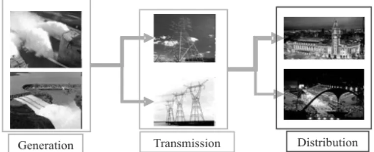
In most of these applications, the linearized repre-sentation (DC) of the power flow has been adopted, due to its bigger simplicity and the degree of satisfactory precision of its results. In the Fig.2 the functional structure of the EPSs are presented.
According to [5], the functional structural components which are presented in the Fig.2 are:
• Generation: formed by generating plants or powerhouses. These powerhouses can be hydroelectric, thermal (coal, oil or natural gas) or nuclear. The hydroelectric power-houses, generally, are located far from the consuming centers, making it necessary to have complex transmission systems and high tension.
• Transmission: constituted by the transmission auxiliary equipments
which are needed to transmit the power produced in the generating powerhouses to the consumers’ centers. The transmission systems can be of alternate current (AC) or continuous current (CC).
• Distribution: constituted by the substations and feeders which are responsible for the electric power distribution to the industrial, commercial and residence consu-mers.
The mathematical model of the OPF problem is represented by an optimizing problem formulated in the next section.
Formulation of the Optimum Power Flow Problem
The optimum power flow problem, as seen before, consists in determining the state of an electric network. It maximizes or minimizes an objective function while it satisfies a group of physical and operational restrictions.
The restrictions of equality correspond to the active and reactive power balance equations in each network’s busbar. The inequalities are functional restrictions, such as flow monitoring in lines and physical and operational limits of the system.
The Optimum Power Flow problem can be formulated mathematically and, generically, by:
(2)
where:
(
z.w.r)
∈
Rn representsthe state, control and disturbance variables respectively; f(x,u,p) represents the performance index of the system; i
(
z.w.r)
=2 represents power flow equations; j(
z.w.r)
≤2represents functional restrictions, in other words, active and reactive power limits in the transmission lines and transformers, reactive power injection limits in the controlling tension bars and injection of active power in the reference bar;
o cz o kp
o cz
o kp
z
z
g
w
w
w
z
≤
≤
≤
≤
represent limits on the state and controlling variables, respectively.
Mathematical Programming Applied in the Optimum Power Flow Problem DC
Initial Considerations An electric power system has a series of controlling devices which have a direct influence on the operational conditions and, therefore, should be included in the modeling of the system so that it can correctly simulate its performance. The table 1 lists each of the cases that were investigated, the
(
)
(
)
(
)
o cz o kp o cz o kp . .000. 3 . 2 . . .000. 3 . 2 . . 0 0 . . 0 o kp w w w z z z t l r w z j o k r w z i c u r w z h l k ≤ ≤ ≤ ≤ = ≤ = =network that was used, the problem in question, the objective function, the problem’s restrictions and the optimizing method that was used.
Source: [4]
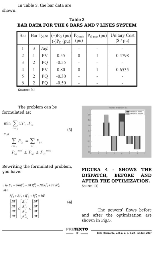
4.2. Economical Dispatch – Case I Case 1 consists in solving an economical dispatch problem using an objective function of which goal it to minimize the cost of the active power generation. The MatLab’s LINPROG routine will be used to solve this case.
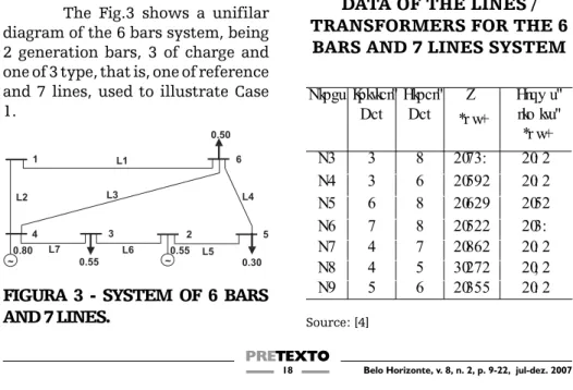
The Fig.3 shows a unifilar diagram of the 6 bars system, being 2 generation bars, 3 of charge and one of 3 type, that is, one of reference and 7 lines, used to illustrate Case 1.
The data for the modeling, resolution and analysis of the problem, are found in the Tables 2 and 3. In the Table 2 the data about the lines are shown.
Table 2
DATA OF THE LINES / TRANSFORMERS FOR THE 6
BARS AND 7 LINES SYSTEM
Nkpgu Kpkvkcn" Dct Hkpcn" Dct Z *r w+ Hnqy u" nko kvu" *r w+ N3 3 8 2073: 20: 2 N4 3 6 20592 20: 2 N5 6 8 20629 2052 N6 7 8 20522 203: N7 4 7 20862 20: 2 N8 4 5 30272 20; 2 N9 5 6 20355 20: 2 Source: [4] Table 1
SYNTHESIS OF THE CASES TO BE INVESTIGATED
FIGURA 3 - SYSTEM OF 6 BARS AND 7 LINES.
In Table 3, the bar data are shown.
Source: [4]
The problem can be formulated as:
(3)
Rewriting the formulated problem, you have: ⎥ ⎥ ⎥ ⎥ ⎦ ⎤ ⎢ ⎢ ⎢ ⎢ ⎣ ⎡ ≤ ⎥ ⎥ ⎥ ⎥ ⎥ ⎦ ⎤ ⎢ ⎢ ⎢ ⎢ ⎢ ⎣ ⎡ ≤ ⎥ ⎥ ⎥ ⎥ ⎦ ⎤ ⎢ ⎢ ⎢ ⎢ ⎣ ⎡ = + + + + + + = 7 0 2 7 0 2 7 0 2 7 0 2 R R R R 2 0 2 2 0 2 2 0 2 2 0 2 57 0 3 R R R R 0 c 0 u R : 0 2 R 3 0 2 R ; 0 2 R 6 0 2 E o kp D 6 I C 6 I D 4 I C 4 I D 6 I C 6 I D 4 I C 4 I D 6 I C 6 I D 4 I C 4 I V
FIGURA 4 - SHOWS THE DISPATCH, BEFORE AND AFTER THE OPTIMIZATION.
The powers’ flows before and after the optimization are shown in Fig.5.
Table 3
BAR DATA FOR THE 6 BARS AND 7 LINES SYSTEM
(4)
Source: [4]
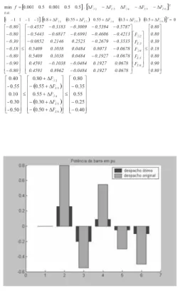
Congestion Management Case II
This case involves conges-tion management with the minimum of load cut. The network data are the same as in Case I. The limits of the controlling variables are described in Table 4. The limits of the power flowes were reduced in 50%, aiming in creating situations of multiple congestions. To solve the problem, the MatLab toolbox optimization from LINPROG routine will be maintained. Table 4 LIMITS IN THE CONTROLLING VARIABLES Controlling Variable Nko kvKphgtkqt""*r w+ Uwr gtkqt" Nko kv"*r w+ RI 4 2062 20: 2 RF 5 /2077 /2057 RI 6 2032 2077 RF 7 /2052 /2047 RF 8 /2072 /2062
The problem can be formuladed in an incremetal form:
The initial and final flowes are represented in Fig.7.
FIGURA 5 - FLOWES IN THE LINES
FIGURA 6 - SHOWS THE CON-TROLLING VARIABLES BEFORE AND AFTER THE SOLUTION OF THE LOAD SHEDDING PROBLEM.
Final Considerations
This paper investigated the mathematic programming appli-cations, more precisely, the linear programming to the linearlized optimum power flow problem.
Different methods of problem solutions in linear pro-gramming were presented and discussed. The interior points method was reported as being indicated for lager problems. The Simplex algorithm showed itself to be adequate for smaller and medium size networks.
The optimum power flow problem, in its several formulations, was examined and its objective functions and typical problems’ restrictions were described.
Formulations of Optimum Dispatch and Network Congestion problems, in its linear version, were presented and numerical
FIGURA 7 – FLOWS IN THE LINES
Source: [4]
demonstrative examples were also presented.
References:
[1] ARAUJO, Leandro Ramos de. Uma Contribuição
ao Fluxo de Potência Ótimo Aplicado a Sistemas de Potência Trifásicos usando o Método dos Pontos Interiores. Tese (Doutorado). COPPE – UFRJ, Rio
de Janeiro, 2005.
[2] BAPTISTA, E. C., at al. Um método primal-dual
aplicado na resolução do problema de fluxo de potência ótimo. Pesquisa Operacional, v.24, n.2,
p.215-226, 2004.
[3] BAZARAA, M.S.; Jarvis, J.J. & Sherali, H.D.
Linear Programming and Network Flows. 2nd Ed.,
Wiley, New York. 1992.
[4] COSTA, Emerson Eustáquio. Elementos de
programação matemática: aplicações ao problema do fluxo de potência ótimo linearizado. 2006. 136 f.
Dissertação (Mestrado) - Pontifícia Universidade Católica de Minas Gerais, Programa de Pós-Graduação em Engenharia Elétrica.
[5] FALCAO, Djalma M.: Análise de Redes Elétricas. COPPE – UFRJ, Rio de Janeiro, 2003.
[6] GOLDBARG, M.C. LUNA, Henrique Pacca L. Otimização combinatória e programação linear:
modelos e algoritmos. 2ª. Edição. Rio de Janeiro:
Elsevier,2005.
[7] LIMA, A.M. de. Comparação entre diferentes
abordagens do problema do fluxo de potência ótimo utilizando o método de pontos interiores. Dissertação
(Mestrado). UCMC-USP, São Paulo, 2004. [8] OLIVEIRA, A.R.L., FILHO, S.S.. Métodos de
pontos interiores para problemas de fluxo de potência ótimo DC. Revista Controle & Automação. Vol. 14
nº 3.2003.
[9] TERRA, L.D.B. A global Methodology for Reactive
Power Management and Voltage Control in Power System. Tese (Doutorado). Imperial College
– London 1989.
[10] WRIGHT, M.H. The interior-point revolution
in optimization: History, recent developments, and lasting consequences. Bulletin of the American
Mathematical Society. Vol. 42, nº 1, p. 39-56. 2004.
Emerson Eustáquio Costa Professor da Universidade FUMEC Mestre em Engenharia Elétrica pela Pontifícia
Universidade Católica de MG Graduado em Matemática pelo Centro
Universitário de Belo Horizonte Endereço para contato Faculdade de Ciências Empresariais - FACE
Universidade FUMEC Rua Cobre nº200 Bairro Cruzeiro 30310-190 - Belo Horizonte – MG
Fone 31 3228 3060 [email protected]
Luiz Danilo Barbosa Terra Professor titular da Pontifícia Universidade
Católica de Minas Gerais
Doutor em Electric Engineering pela University of London
Mestre em Engenharia Elétrica pela Universidade Federal de Minas Gerais
Endereço para contato Avenida Dom José Gaspar, 500 Coração
Eucarístico.
30535-901 - Belo Horizonte - MG Telefone: (31) 3319.4444 Fax: (31)
3319.4225 [email protected]
George Leal Jamil Professor do programa de Mestrado
em Administração Universidade FUMEC Doutor em Ciência da Informação pela
Universidade Federal de Minas Gerais Mestre em Ciência da Computação pela
Universidade Federal de Minas Gerais Endereço para contato
Avenida Afonso Pena nº3880 - Bairro Cruzeiro 30130 - 009 - Belo Horizonte – MG
Fone 31 3223 8033 [email protected]