External dependency, value added generation and structural change: an interindustry approach

João Ferreira do Amaral, João Carlos Lopes* & João Dias

External dependency, value added generation and

structural change: an interindustry approach

WP 12/2010/DE/UECE

___________________________________________________________________

Department of Economics

W

P

ISSN Nº 0874-4548

School of Economics and Management

External dependency, value added generation and

structural change: an interindustry approach

João Ferreira do Amaral, João Carlos Lopes* and João Dias ISEG (School of Economics and Management) - Technical University of Lisbon,

and UECE (Research Unit on Complexity and Economics)

Abstract

The external dependency of many industries and the corresponding low value added generated in production create high external deficits and growing debt to GDP ratios in several open economies. In this paper we propose an empirical method to assess the evolution of these vulnerabilities, based on a new treatment of interindustry production multipliers. The (gross) output growth potential given by the column sums of the Leontief inverse matrix (backward linkage indicators) results from three terms: interindustry consumptions, value added and imported inputs. After a convenient arrangement of these terms, the evolution of backward linkage indicators can be used to detect structural changes, particularly quantifying a (net) growth effect (more value-added generation) and an external dependency effect (more imported inputs), and to classify the productive sectors accordingly. An application to the Portuguese Economy is made, using input-output tables for the years 1980, 1995 and 2005. This method can also be useful as a simple, but suggestive, device to compare the evolution of two or more economies, along their development processes in time.

Keywords: input-output linkages, external dependency, structural change, Portugal JEL classification: C67, D57

* Corresponding author: ISEG - Rua Miguel Lupi, nº 20, 1249-078 Lisboa, Portugal. E-mail address: [email protected]

______________________

The financial support of FCT (Fundação para a Ciência e a Tecnologia), Portugal, is gratefully

1. Introduction

The external dependency of many industries (strong reliance on imported inputs) and

the associated low value added generated in domestic production are important

vulnerabilities in several developed and developing open economies. When associated

with a relatively high level of personal consumption and a weak export potential, they

tend to create high external deficits and a rapidly growing debt to GDP ratio that

request very demanding financial efforts and disturbing macroeconomic imbalances.

In this paper we propose an empirical method to evaluate the changes in the external

dependency of the production system of an economy and its capacity to generate value

added, based on a new treatment of interindustry production multipliers.

The column sums of the Leontief inverse matrix (backward linkage indicators) give the

output growth of all sectors when the final demand directed to each (correspondent)

sector increases by one unity, and this growth potential can be divided in three terms:

interindustry flows, value-added and imported inputs (a good exposition of the basic

structure and results of the Leontief model is made in Miller and Blair, 2009).

After a convenient arrangement of these terms, the evolution of backward linkage

indicators can be used to detect structural changes, particularly quantifying a (net)

growth effect (more value-added) and an external dependency effect (more imported

inputs), and to classify the productive sectors accordingly.

An application to the Portuguese economy is made for the period 1980-2005, divided in

Portuguese version: 1977; and 1995-2005, with data for 60 sectors, based on the E.U.

SEC1995. This method can also be useful as a simple, but suggestive, device to

compare the evolution of two or more economies.

Since the pioneering work of Rasmussen (1956) and Hirschman (1958), the concepts of

backward and forward linkages have been widely discussed and applied (for an

interesting survey and discussion see Drejer, 2002).

More recently, sophisticated methods to deal with structural change have been

proposed (Sonis et al (1995), Dietzenbacher and van der Linden (1997), Dridi and

Hewings (2002), are, among others, very interesting examples).

The strategy in this work is different, and based on the conviction that sometimes,

‘back to basics’ and simplicity enriched with easy visualisation ways to look at the data

can play an important role in our understanding of how an economy evolves in time.

2. Interindustry linkages indicators

The Rasmussen traditional method of using compact indicators from the production

multipliers matrix (Leontief inverse) is one of the classical references for the analysis of

intersectoral relations.

It is well known that this matrix is obtained by solving an n equations system that

equates sector productions to possible uses: intermediate and final demand.

This system can be represented as follows:

(2.1) x = A x + y,

with: A – (domestic) technical coefficients matrix; x – sectoral production vector; y –

(domestic) sectoral final demand vector.

The solution of this system is:

(2.2) x = B y, with B = (I-A)-1

Each element of B is a production multiplier that gives the total (direct and indirect)

effect in one’s sector production of a unity increase in domestic final demand of a given

sector. That is, bij is the global impact on the sector i production when the domestic final

demand of sector j increases by one unity.

Particular interest in this context has the notion of backward linkage indicators:

(2.3)

∑

=

= n i

ij

j b

b

1

0 ( j = 1, … , n )

This indicator results from summing up the n values of column j and gives the effect on

total production (of all sectors) of a unitary change in the final demand directed to j

sector. The larger the value of this coefficient, the larger will be the impact of this

increase of the final demand on the sector concerned and on all the others. For the

method we propose in the next section and its empirical application to the Portuguese

3. Net growth (or efficiency

)

and external dependency effects

The backward linkage indicators can be used to evaluate the gains in the capacity of an

economy to generate value added and the changes in external dependency of an

economy from one year to another.

The overall effect of a unity change of final demand is the sum of three terms:

interindustry flows, value added and imported inputs.

Moreover, an important property applies: the second and last terms sum up unity,

exactly the value of the initial (exogenous) stimulus, and this is so because in

equilibrium the total value of sectoral final demand equals the gross value added plus

imported inputs of all sectors.

Using this property, and after a convenient arrangement of terms, the evolution of

backward linkage indicators, value added and imported input coefficients over time can

be used to detect structural changes in the economy.

Particularly, we can quantify the capacity to generate more (or less) value-added by

unity of final demand (what in some sense we can call an ‘efficiency effect’, although a

peculiar one1), and the need to import more (or less) intermediate inputs (a certain kind

of ‘external dependency effect’). And we can classify the productive sectors according

1

to the particular combination of both effects, finding a new kind of “key sectors”, those

presenting a positive “efficiency” change and a negative “dependency” change.

One way to express formally these ideas is as follows.

Considering a unitary increase in j sector’s final demand, ∆ yj = 1, its effects on total

production are:

(3.1) Σi ∆xi = Σibij = b0j

By the equilibrium condition between total sectoral final demand and total primary

inputs, we have:

(3.2) ∆ yj = 1 => ∆ (Σi vi +Σi mi) = 1,

where vi and mi are the value added and the value of imported inputs used by sector i.

Defining, and assuming as constants, the value-added coefficients (avi = vi/xi) as well as

the imported inputs coefficients (ami = mi/xi), we have:

(3.3) 1 = Σibij avi + Σibij ami

Dividing both sides of (3.3) by b0j:

and, representing by v*j and m*j the terms in the right hand side of (3.4) (the weighted

average of value-added and imported inputs coefficients, respectively), we arrive finally

at:

(3.5) 1 = b0j (v*j + m*j).

This expression can be used in a dynamic (or, as in the present paper, in a comparative

static) exercise to detect and quantify the changes in the productive structure of an

economy.

Suppose that, for each sector j, we have, between two given years, a decrease inb0j.

This means that, in order to satisfy a unitary increase in sector j final demand it is

necessary a smaller increase in the global production of the economy.

It is also true that, in this case, we must have ∆m*j+∆v*j > 0, and so four situations are

possible, in a two dimensional space with axes ∆v*j and ∆m*j:

- when ∆ v*j > 0 and ∆ m*j < 0, the decrease in b0j goes with a larger capacity to

generate value added (a beneficial ‘net’ growth effect) and a lower necessity of

imported inputs (a reduced external dependency effect) – let’s call this area A, the most virtuous one;

- if ∆v*j > 0, ∆m*j > 0 and ∆v*j/∆ m*j > 1, there is a simultaneous increase in ‘net

growth effect’ and ‘external dependency’, with the first dominating the second (area B);

- with ∆m*j > 0, ∆ v*j > 0, but ∆m*j/∆ v*j > 1, the increase in ‘external dependency’

is relatively more significant than the increase in ‘net growth effect’ (area C);

- finally, with ∆m*j > 0 and ∆ v*j < 0, the decrease in b0j is totally due to an increase

in ‘external dependency’, with a simultaneous decrease in the capacity to generate

value added (area D, the most disadvantageous situation).

For the case of a b0j increase we must have ∆m*j+∆v*j < 0, a worse situation for the

economy, at least from the ‘capacity to generate more value added’ point of view. The

four possible areas now are (in a descending order):

- Area A’: ∆v*j > 0 and ∆ m*j < 0, with ∆ v*j < |∆m*j|

- Area B’: ∆v*j < 0 and ∆ m*j < 0, with |∆ v*j| < |∆m*j|

- Area C’: ∆v*j < 0 and ∆ m*j < 0, with |∆ v*j| > |∆m*j|

- Area D’: ∆v*j < 0 and ∆ m*j > 0, with |∆ v*j| > ∆m*j

In practical terms, a suggestive way of analysis is the graphical presentation of ∆v*j and

∆ m*j values in the two-dimensional space above described, distributing the position of

the sectors in the possible areas A, B, C, D (for a b0j decrease) and A’, B’, C’, D’ (for a

b0j increase). The structural change is more beneficial to an economy when more sectors

4. Application to the Portuguese Economy

We have applied the method presented above to the Portuguese economy in two

periods: 1980-1995 and 1995-2005, using the Domestic Input-Output Tables with 49

sectors (SCNP1977) and 60 sectors (SEC1995), respectively. In both cases the data

sources are Statistics Portugal (INE) and Departamento de Prospectiva e Planeamento

(DPP).

The main conclusion drawn from the results is the apparent global deterioration of the

Portuguese productive system between 1980 and 2005.

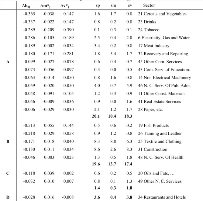
For the first sub-period we can see in tables 1 and 2 that there are in both sub-periods

more sectors with b0j increasing than with b0j decreasing.

< Table 1 approximately here > < Table 2 approximately here >

For the sectors with decreasing b0j only 13 are located in the most virtuous area A (more

‘net growth effect’ and lower external dependency). Moreover, the majority of these

sectors are services, utilities or protected sectors.

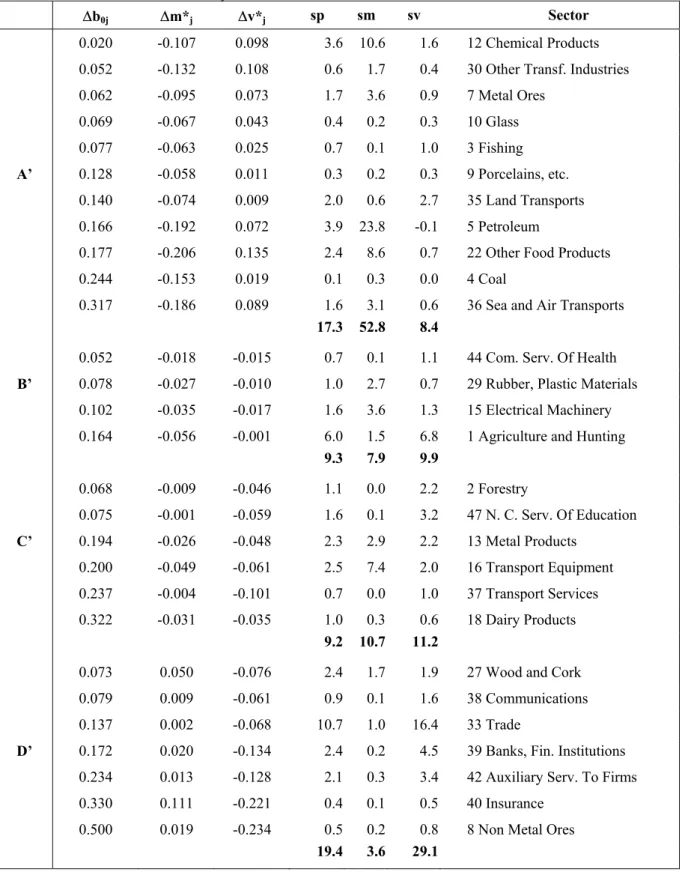
Among the sectors with increasing b0j, only 11 are in the area with positive variation of

These results can be better visualised in Figures 1 and 2. It could be expectable that, as

an economy develops over time most sectors should be concentrated in virtuous areas A

and A’.

< Figure 1 approximately here > < Figure 2 approximately here >

In fact, it is not what we get in this case and it is difficult to explain these findings for

the evolution of the Portuguese productive structure between 1980 and 1995. It was a

period of normalisation of political, economic and social conditions, of economic

integration in the (then) European Economic Community (since 1986) and of relatively

strong growth and real convergence at macroeconomic level.

However, it is important to note that this analysis was made using data at current prices

and therefore the methodology used does not allow us to reach conclusions about the

breakdown of the effects between price effects and technological or other real effects.

Although we have not in Portugal domestic flows input-output data at constant prices,

there are nonetheless good reasons to support the view that the kind of effects that we

tried to measure should in fact be measured at current prices as we have actually done.

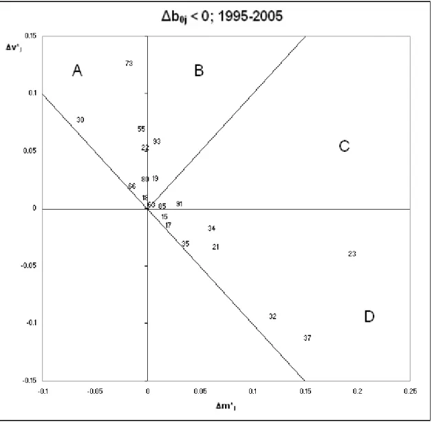
For the second and more recent sub-period, 1995-2005, the tendency for more sectors

with b0j increasing than decreasing remains (see Tables 3 and 4), and the percentage of

sectors in virtuous areas (A and A’) is even smaller (see Figures 3 and 4), representing

around 20% of gross output (against 37,4% in 1980-95) and value added (26,7% in

disadvantage areas (D + D’), from 23% to 51% in terms of production, and from 33% to

48% in terms of value added.

< Table 3 approximately here > < Table 4 approximately here > < Figure 3 approximately here > < Figure 4 approximately here >

However, there is at least one positive tendency in the structural evolution of the

Portuguese productive system concerning the sectoral composition of virtuous areas A

and A’. In 1980-95 there is a clear predominance of services, nontradables or low

technology sectors (Tobaco, Electricity, gas and water, Recovery and repairing, Cereals

and vegetables, Drinks, Commercial Services of Education, Other Commercial

Services, etc.). In 1995-2005 enter in these areas of great value added creation and

lower external dependency several medium and high technology sectors as Office

machinery, R&D services, Machinery and equipment, Fabricated metal products,

Wearing apparel, Other business services. It would be very important to keep these

sectors in virtuous areas and reinforce significantly its weight in the Portuguese

productive system. This can be a valuable contribution to solve (or at least diminish) the

external and macroeconomic imbalances currently affecting the growth performance of

5. Concluding remarks

In this paper we have proposed a simple method to study the structural changes of an

economy, using the traditional Rasmussen indicators based on the production

multipliers matrix or Leontief inverse. This method is appropriate to assess the external

dependency of industries (strong reliance on imported inputs) and the associated low

value added generated in domestic production, an important vulnerability in several

open economies.

We used the method to analyse the evolution of the Portuguese productive structure

between 1980 and 2005, divided in two sub-periods, until and post-1995. Our results

point to a mixed pattern, with the positive gains in the capacity to generate value added

and importing less intermediate inputs overcome by many losses and an increased

external dependency for the majority of sectors, particularly in more recent years.

However, our results also point to an apparent upgrade of the Portuguese productive

system with more medium and high technology sectors entering in the virtuous areas of

value added generation and less dependency.

External dependency is not necessarily bad. It may be the result of increased benefits

from international division of labour. What is not a priori desirable is that the decrease

in production needed to satisfy an increase in domestic demand should be a

consequence of domestic production being supplanted by imports.

One of the possible explanations for the results obtained is the great variation in the

a concept of multiplier that is immune to that variation: the singular value

decomposition method proposed in Ciaschini (1993).

It is important to emphasise that, although conditioned by the well-known limitations of

the traditional gross multipliers (Oosterhaven and Stelder, 2002), the method we

propose can be used as a simple, but (visually) suggestive, device to quantify the

structural changes of an economy. And with some refinements it can also be useful to

compare the evolution of two or more economies along their development paths.

REFERENCES

Ciaschini M. (1993) Modelling the Structure of the Economy (London, Chapman and

Hall).

Dietzenbacher, E. & van der Linden, J. (1997), Sectoral and Spatial Linkages in the EC

Production Structure, Journal of Regional Science, 37, pp. 235-257.

DPP (2001), Estimação de um sistema de matrizes na óptica da produção efectiva,

Documento de Trabalho, Departamento de Prospectiva e Planeamento, Maio.

Drejer, I. (2002), Input-Output Based Measures of Interindustry Linkages Revisited – A

Survey and Discussion, Paper presented at the 14th International Conference on

Input-Output Techniques, Montreal, Canada.

Dridi, C. & Hewings, G. (2002) An Investigation of Industry Associations, Association

Loops and Economic Complexity: Application to Canada and the United States,

Hirschman, A. (1958) The Strategy of Economic Development (New York, Yale

University Press).

INE, Contas Nacionais, Lisboa.

Miller, R. E. and Blair, P. D. (2009), Input-Output Analysis: Foundations and

Extensions, Second edition. New York: Cambridge University Press.

Oosterhaven, J. & Stelder, D. (2002), Net Multipliers Avoid Exaggerating Impacts:

With a bi-regional illustration for the Dutch transportation sector, Journal of

Regional Science, 42, pp. 533-43.

Rasmussen, P. (1956) Studies in intersectoral relations (Amsterdam, North-Holland).

Sonis, M., Hewings, G. & Guo, J. (1996) Sources of structural changes in input-output

systems: a field of influence approach, Economic Systems Research, 8, pp. 15-32.

Annex: Tables and Figures

Table 1: Negative variation of b0j, 1980-95

∆b0j ∆m*j ∆v*j sp sm sv Sector

-0.365 -0.038 0.147 1.6 1.7 0.8 21 Cereals and Vegetables -0.337 -0.022 0.147 0.8 0.2 0.8 23 Drinks

-0.289 -0.209 0.390 0.1 0.3 0.1 24 Tobacco

-0.286 -0.105 0.189 2.5 0.4 2.0 6 Electricity, Gas and Water -0.189 -0.002 0.034 3.4 0.2 0.8 17 Meat Industry

-0.180 -0.171 0.281 1.8 3.4 1.7 32 Recovery and Repairing A -0.099 -0.027 0.078 0.6 0.4 0.7 45 Other Com. Services

-0.073 -0.056 0.097 0.3 0.0 0.5 43 Com. Serv. of Education. -0.063 -0.014 0.050 0.8 1.6 0.8 14 Non Electrical Machinery -0.059 -0.020 0.050 4.0 0.7 5.9 46 N. C. Serv. Of Pub. Adm. -0.048 -0.091 0.105 1.2 0.3 0.9 11 Other Const. Materials -0.046 -0.009 0.036 0.9 0.0 1.6 41 Real Estate Services -0.006 -0.029 0.030 2.1 1.2 1.7 28 Paper, etc.

20.1 10.4 18.3

-0.513 0.055 0.144 0.5 0.6 0.2 19 Fish Products -0.218 0.029 0.058 0.9 1.2 0.8 26 Tanning and Leather B -0.171 0.018 0.040 8.3 8.8 6.3 25 Textile and Clothing

-0.130 0.011 0.034 8.6 2.6 8.3 31 Construction

-0.046 0.003 0.023 1.3 0.5 1.8 48 N. C. Serv. Of Health

19.6 13.7 17.4

C -0.118 0.039 0.002 0.6 0.2 0.5 20 Oils and Fats, … -0.032 0.010 0.007 0.8 0.1 1.3 49 Other N. C. Services

1.4 0.3 1.8

Table 2: Positive variation of b0j, 1980-95

∆b0j ∆m*j ∆v*j sp sm sv Sector

0.020 -0.107 0.098 3.6 10.6 1.6 12 Chemical Products 0.052 -0.132 0.108 0.6 1.7 0.4 30 Other Transf. Industries 0.062 -0.095 0.073 1.7 3.6 0.9 7 Metal Ores

0.069 -0.067 0.043 0.4 0.2 0.3 10 Glass 0.077 -0.063 0.025 0.7 0.1 1.0 3 Fishing A’ 0.128 -0.058 0.011 0.3 0.2 0.3 9 Porcelains, etc.

0.140 -0.074 0.009 2.0 0.6 2.7 35 Land Transports 0.166 -0.192 0.072 3.9 23.8 -0.1 5 Petroleum

0.177 -0.206 0.135 2.4 8.6 0.7 22 Other Food Products 0.244 -0.153 0.019 0.1 0.3 0.0 4 Coal

0.317 -0.186 0.089 1.6 3.1 0.6 36 Sea and Air Transports

17.3 52.8 8.4

0.052 -0.018 -0.015 0.7 0.1 1.1 44 Com. Serv. Of Health B’ 0.078 -0.027 -0.010 1.0 2.7 0.7 29 Rubber, Plastic Materials

0.102 -0.035 -0.017 1.6 3.6 1.3 15 Electrical Machinery 0.164 -0.056 -0.001 6.0 1.5 6.8 1 Agriculture and Hunting

9.3 7.9 9.9

0.068 -0.009 -0.046 1.1 0.0 2.2 2 Forestry

0.075 -0.001 -0.059 1.6 0.1 3.2 47 N. C. Serv. Of Education C’ 0.194 -0.026 -0.048 2.3 2.9 2.2 13 Metal Products

0.200 -0.049 -0.061 2.5 7.4 2.0 16 Transport Equipment 0.237 -0.004 -0.101 0.7 0.0 1.0 37 Transport Services 0.322 -0.031 -0.035 1.0 0.3 0.6 18 Dairy Products

9.2 10.7 11.2

0.073 0.050 -0.076 2.4 1.7 1.9 27 Wood and Cork 0.079 0.009 -0.061 0.9 0.1 1.6 38 Communications 0.137 0.002 -0.068 10.7 1.0 16.4 33 Trade

D’ 0.172 0.020 -0.134 2.4 0.2 4.5 39 Banks, Fin. Institutions 0.234 0.013 -0.128 2.1 0.3 3.4 42 Auxiliary Serv. To Firms 0.330 0.111 -0.221 0.4 0.1 0.5 40 Insurance

0.500 0.019 -0.234 0.5 0.2 0.8 8 Non Metal Ores

Table 3. Negative variation of b0j, 1995-2005

∆b0j ∆m*j ∆v*j sp sm sv Sector

-0.237 -0.018 0.126 0.2 0.0 0.2 73 Research and development services -0.226 -0.006 0.069 3.7 2.6 2.7 55 Hotel and restaurant services -0.153 -0.002 0.053 1.1 1.6 0.8 22 Printed matter and recorded media A -0.033 -0.002 0.025 3.6 0.4 6.3 80 Education services

-0.030 -0.064 0.077 0.1 0.4 0.1 30 Office machinery and computers -0.023 -0.002 0.009 2.6 4.5 1.5 18 Wearing apparel; furs

-0.008 -0.015 0.019 0.7 0.2 0.8 66 Insurance and pension funding services

12.0 9.7 12.4

B -0.149 0.009 0.058 0.5 0.2 0.7 93 Other services

-0.098 0.007 0.026 1.6 3.3 1 19 Leather and leather products

2.1 3.5 1.7

C -0.148 0.03 0.004 0.4 0.2 0.2 91 Membership organisation services n.e.c. -0.034 0.014 0.002 4.2 2.1 5.4 85 Health and social work services

-0.02 0.004 0.003 0.9 0.2 1.1 63 Supp./ aux. transport serv.; travel agency serv.

5.5 2.5 6.7

D -0.226 0.195 -0.04 1 7.4 -0.1 23 Coke, refined petrol. prod. and nuclear fuels -0.116 0.152 -0.113 0.1 0 0.1 37 Secondary raw materials

-0.1 0.065 -0.034 1.6 1.8 1.1 21 Pulp, paper and paper products

-0.094 0.061 -0.018 1.6 7 0.5 34 Motor vehicles, trailers and semi-trailers -0.045 0.119 -0.094 0.8 3.8 0.3 32 Radio, televi., comm. equip. and apparatus -0.035 0.016 -0.008 6.8 9.3 2.9 15 Food products and beverages

-0.012 0.02 -0.015 3 5.3 2.3 17 Textiles

-0.01 0.036 -0.031 0.4 0.7 0.4 35 Other transport equipment

15.3 35.3 7.5

Table 4. Positive variation of b0j, 1995-2005

∆b0j ∆m*j ∆v*j sp sm sv Sector

A’ 0.007 -0.019 0.017 5.8 3.4 5.5 74 Other business services

0.013 -0.079 0.074 1.2 4.1 0.5 29 Machinery and equipment n.e.c. 0.041 -0.043 0.030 1.0 3.0 0.4 28 Fab. metal prod., except mach. and equip.

8.0 10.5 6.4

B’ 0.034 -0.013 -0.002 2.8 2.6 3.4 50 Trade, maint., repair serv. of motor vehicles

2.8 2.6 3.4

C’ 0.008 -0.002 -0.003 4.1 0.3 6.5 70 Real estate services

0.114 -0.015 -0.036 0.3 0.1 0.4 67 Services auxiliary to financial intermediation 0.120 0.000 -0.043 6.0 2.8 7.0 51 Wholesale trade

0.120 0.000 -0.048 3.1 0.9 4.0 52 Retail trade services

0.143 -0.003 -0.050 2.1 5.9 1.3 24 Chemicals, chemical products

0.161 -0.005 -0.068 0.1 0.0 0.2 90 Sewage, refuse disposal services, sanitation 0.179 -0.008 -0.089 2.8 0.7 4.5 65 Financial interm. services, except insurance

18.5 10.7 23.9

D’ 0.036 0.028 -0.038 1.9 1.5 1.5 26 Other non-metallic mineral products 0.052 0.006 -0.025 0.9 2.2 0.5 25 Rubber and plastic products

0.056 0.028 -0.050 0.3 0.0 0.4 41 Collected and purified water, distr. water 0.058 0.001 -0.022 1.5 0.7 1.7 92 Recreational, cultural and sporting services 0.067 0.009 -0.031 1.1 2.2 0.8 36 Furniture; other manufactured goods n.e.c.

0.073 0.010 -0.066 0.5 0.0 0.9 2 Forestry 0.077 0.024 -0.063 0.3 0.1 0.4 5 Fish

0.084 0.027 -0.063 1.1 2.9 0.8 31 Electrical machinery and apparatus n.e.c. 0.086 0.006 -0.027 9.3 5.4 7.2 45 Construction work

0.087 0.031 -0.068 0.2 0.4 0.2 33 Medical, precision, optical instrum. 0.095 0.128 -0.167 0.8 1.6 0.7 27 Basic metals

0.105 0.026 -0.060 3.2 1.1 3.7 1 Agriculture, hunting

0.141 0.020 -0.079 0.4 0.1 0.6 72 Computer and related services 0.142 0.004 -0.095 4.5 0.9 7.8 75 Public admin., defence, social security

0.145 0.019 -0.056 1.3 1.3 0.9 20 Wood, cork 0.150 0.065 -0.134 0.1 0.1 0.1 16 Tobacco

0.165 0.025 -0.073 0.3 0.2 0.3 61 Water transport services 0.177 0.025 -0.122 0.1 0.0 0.2 13 Metal ores

0.192 0.041 -0.105 0.3 0.1 0.3 14 Other mining and quarrying 0.247 0.075 -0.164 0.6 0.9 0.6 62 Air transport services

0.260 0.093 -0.166 3.2 1.9 3.1 40 Electrical energy, gas, steam and hot water 0.265 0.006 -0.114 1.7 1.0 2.2 64 Post and telecommunication services 0.270 0.026 -0.161 0.7 0.1 1.1 71 Renting services of mach. and equipment

0.288 0.046 -0.167 1.5 0.4 2.1 60 Land transport; transport via pipeline

Figure 1: Negative variation of b0j, 1980-95.

-0.3 -0.2 -0.1 0 0.1

-0.1 0 0.1 0.2 0.3 0.4 0.5 24 32 6 11 ₄₃ 21 28 45 23 4614 4117 48 49 31 34 2526 20 19

∆ m*j

∆ v*j

∆b0j < 0; 1980-95

A

_B

C

Figure 2: Positive variation of b0j, 1980-95

-0.25 -0.15 -0.05 0.05 0.15

-0.3 -0.2 -0.1 0 0.1 0.2 0.3 22 536 4 30 12 7 35 10 3 9 1 16 15 18 29 13 44 2 37 47₃₃₃₈ 42 8 39 27 40

∆ m*j

∆v*j

∆b0j > 0; 1980-95

A’

B’