Propagation model for cellular mobile networks used in UAVcommunications environmentss

(1)

Departamento de Ciências e Tecnologias de Informação

Propagation model for cellular mobile networks used in UAVs

communications environments

André de Sousa Silvério

Dissertação submetida como requisito parcial de obtenção do grau de

Mestre em Engenharia de Telecomunicações e Informática

Orientador:

Prof. Pedro Joaquim Amaro Sebastião, Professor Auxiliar, ISCTE-IUL

Co-orientador: Prof. Alexandre Almeida, Professor Auxiliar, ISCTE-IUL

(2)

(3)

III

ABSTRACT

Recognizing the growth of the drone market in recent years, it is crucial to evaluate the capacity of the mobile communications technologies as well as their infrastructure to verify if these are capable to support various applications and services that may associate with these type of vehicles, achieving lower costs to the users. The type of application chosen for this thesis is a video streaming that is able to assume different qualities depending on the RF conditions, in order to overcome the limitation of radio communications, in which the user is only able to communicate with the drone when in his line of sight.

It was necessary to take into account a propagation model that considered the unique characteristics of an UAV, since the most commonly used models only consider a typical mobile user moving below the level of the BSs and their respective antennas using a short/medium frequency interval that is not able to consider the third and fourth generation technologies at once. In order to choose the ideal model, a theoretical study was carried out, which allowed to conclude that Lisbon University Institute Model is the most accurate since it is able to fulfill the requirements associated to a flying drone, considering a larger frequency spectrum, allowing the use of third and fourth generation technologies that are fundamental to support multimedia services, such as video streaming.

To verify the viability of mobile communications, measurements were made in three real scenarios in rural areas using a spectrum analyzer carried by a flying drone, in order to monitor, read and write the data related to the signal’s behavior into a file, during the flight route.

Based on this approach, it was possible to analyze the viability of mobile communications for a video streaming service using a drone, in a rural environment and considering UMTS and LTE technologies. In addition, evaluate the signal’s performance when the drone is above the antennas where the “hole phenomenon” occurs, theoretically.

Keywords: Cellular/Wireless Networks, Mobile Communications, UAV, Propagation

(4)

IV This page was intentionally left in blank

(5)

V

RESUMO

Tendo em conta o crescimento que o mercado de drones tem tido nos últimos anos, é importante considerar as tecnologias de comunicações móveis assim como as respectivas infraestruturas e verificar se estas são capazes de suportar diversas aplicações que podem estar associadas a estes veículos, permitindo isto um custo inferior para os utilizadores dos mesmos. O tipo de aplicação escolhida para esta tese foi uma streaming de vídeo, com o objetivo de ultrapassar a limitação das comunicações rádio, em que o utilizador apenas consegue comunicar com o drone caso este se encontre no seu campo de visão. Foi necessário ter em conta um modelo de propagação que considerasse as características únicas de movimentação dum drone, uma vez que os modelos mais utilizados apenas consideram um utilizador móvel comum que se desloque abaixo do nível das estações base e respetivas antenas para um espectro de frequências curto/médio. Para a escolha deste modelo, foi realizado um estudo teórico que permitiu concluir que o Lisbon University Institute Model é o mais acertado, uma vez que é capaz de cumprir os requisitos associados a um drone, considerando um intervalo de frequências maior, permitindo a utilização das tecnologias de terceira e quarta geração, que são fundamentais para suportar aplicações multimedia, como é o caso da streaming de vídeo. Para verificar a viabilidade das comunicações móveis, foram feitas medições em três cenários reais em zona rural recorrendo a um analisador de espectros transportado por um drone, com o objetivo de monitorizar, fazer a leitura e gravação de dados associados ao comportamento do sinal para um ficheiro durante a rota de voo.

Com esta abordagem, foi possível analisar a viabilidade das comunicações móveis para a aplicação de streaming de vídeo num drone, em cenário rural, considerando as tecnologias UMTS (3G) e LTE (4G). Para além disso, foi ainda possível avaliar o comportamento do sinal quando o drone se encontra acima do eixo vertical das antenas, onde o “fenómeno do buraco” ocorre.

Palavras-chave: Redes celulares, Comunicações móveis, Modelos de propagação, LTE,

(6)

VI This page was intentionally left in blank

(7)

VII

ACKNOWLEDGMENTS

I will take this opportunity to express my gratitude to my supervisor Prof. Pedro Sebastião for the support, patience, motivation, availability and shared knowledge throughout the year. His guidance helped me to follow the correct path with the right thoughts, the correct attitude and without his help, I wouldn’t be able to reach the right persons and companies to supply the necessary instruments for this thesis.

Furthermore, I would like to give a special thanks to Eng. Ricardo Freitas from Rohde & Schwarz, for trusting me and giving me the responsibility to take care of an expensive instrument since without it, I wouldn’t be able to get such reliable results.

I would like to thank my colleague, Ricardo Silva, for providing a drone capable of lifting the spectrum analyzer and for all the effort on preparing, adjusting and controlling it to recreate a real-world scenario, in order to obtain a successful measurement campaign. Also, I would like to thank António Raimundo from IT for the interest and availability to help me and Ricardo S. during the measurements week.

At last, but not least, I would like to thank my loved ones, specially my mom, who kept me motivated and focused during my academic path.

(8)

VIII This page was intentionally left in blank

(9)

IX

CHAPTER 1 INTRODUCTION ... 1 1.1 Overview ... 2 1.2 Motivation ... 3 1.3. Objectives ... 4 1.4. Contributions ... 5 1.5. Dissertation Structure ... 5 CHAPTER 2 CONCEPTS ... 7 2.1 Cellular Networks ... 8 2.1.1 GSM ... 9 2.1.2 UMTS ... 12 2.1.3 LTE ... 13 2.1.3 Handover ... 15 2.2. Drone ... 18 2.3. Spectrum Analyzer ... 19 2.4. Frequency bands ... 21

CHAPTER 3 PROPAGATION MODELS AND PROPOSED MODEL ... 22

3.1. Overview ... 23

3.2. Propagation models ... 23

3.2.1. Okumura Model ... 23

3.2.2. Hata Model ... 28

3.2.3. Cost 231-Hata Model... 29

3.2.4. COST 231 – Walfish-Ikegami Model ... 30

3.2.5. Erceg Model (or basic SUI model) ... 31

3.2.6. LUI Model ... 33

CHAPTER 4 MEASUREMENTS ... 40

4.1. Overview ... 41

4.2. Measurement campaign requirements ... 43

4.3. Locations and flight routes ... 45

4.4. Measurement results ... 48

4.4.1. Scenario A ... 52

(10)

X

4.4.3. Scenario C ... 65

CHAPTER 5 CONCLUSIONS ... 71

5.1. Main conclusions ... 72

5.2 Future Work ... 74

ANNEX A ROMES SOFTWARE ... 76

ANNEX B MEASUREMENT RESULTS ... 93

B.1. Scenario A: ... 94  LTE (796 MHz Channel) ... 94  UMTS (2152.4 MHz Channel): ... 96  UMTS (2157.4 MHz Channel): ... 97 B.2. Scenario B: ... 99  LTE (796 MHz Channel): ... 99  UMTS (2152.4 MHz Channel): ... 101 B.3. Scenario C: ... 103  LTE (806 MHz Channel): ... 103  UMTS (2117.8 MHz Channel): ... 106

ANNEX C ADDITIONAL STATISTIC ... 108

Overview ... 109 C.1. Scenario A ... 109 LTE ... 109 UMTS ... 113 C.2. Scenario B ... 117 LTE ... 117 UMTS ... 120 C.3. Scenario C ... 123 LTE ... 123 UMTS ... 126 REFERENCES ... 130

(11)

XI

TABLE OF FIGURES

Figure 2- 1. Cellular Networks technologies evolution, Source: [4] ... 9

Figure 2- 2. GSM Coverage Worldwide, Source: [5] ... 10

Figure 2- 3. GSM Architecture, Source: [6] ... 11

Figure 2- 4. UMTS Architecture, Source: [8] ... 12

Figure 2- 5. Network infrastructure from GSM to LTE, Source: [11] ... 14

Figure 2- 6. OFDMA (DL) and SC-FDMA (UL), Source: [11] ... 14

Figure 2- 7. Hard Handover, Source: [13] ... 16

Figure 2- 8.Soft Handover, Source: [13] ... 17

Figure 2- 9. Softer Handover, Source: [13] ... 17

Figure 2- 10. Inter-LTE/RAT Handover, Source: [15] ... 18

Figure 2- 11. Intra-LTE Handover, Source: [15] ... 18

Figure 2- 12.Octocopter (drone) with TSMA attached (under it) ... 19

Figure 2- 13. Spectran HF-60100, Source: [16] ... 19

Figure 2- 14. R&S TSME scanner connected to a PC, Source: [18]... 20

Figure 2- 15. R&S TSMA scanner and TSMA-BP (battery pack), Source: [20] ... 21

Figure 3- 1 - Median attenuation related to free space (Okumura model), Source: [23] ... 25

Figure 3- 2. BS Effective Height gain, Source: [23] ... 25

Figure 3- 3. Mobile height gain factor, Source: [23] ... 26

Figure 3- 4. Correction factor for different types of terrain, Source: [23] ... 27

Figure 3-5. Rectangular function, Source: [1] ... 35

Figure 3-6. Unit step function, Source: [1] ... 36

Figure 3-7. Angles associated to the antenna, Source: [1] ... 37

Figure 3-8. Sectorial choice and identification, Source: [1] ... 38

Figure 4- 1. Proposed flight plan: X(distance) and Y(altitude) axes ... 41

Figure 4-2. R&S TSMA accessories, Source: [32] ... 43

Figure 4-3. R&S TSMA - Rear Panel, Source: [32] ... 43

Figure 4-4. R&S TSMA and TSMA-BP with some accessories connected, Source: [32]... 44

Figure 4-5. Equipment attached below the drone with velcro tape ... 44

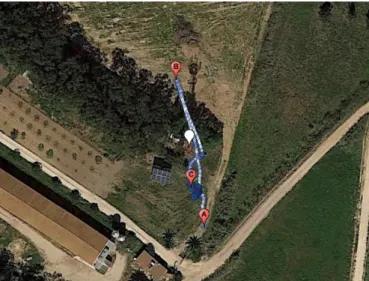
Figure 4-6. Base Station A (MEO) ... 45

Figure 4-7. Scenario A (BS A) and respective flight route ... 46

Figure 4-8. Scenario B (BS A) and respective flight route ... 46

Figure 4-9. Base Station B (Vodafone) ... 47

Figure 4-10. Scenario C and respective flight route ... 48

Figure 4-11. 5 MHz channels UMTS Band I (DL) ... 51

Figure 4-12. 10 MHz channels LTE Band 20 ... 51

Figure 4-13. 20 MHz channels LTE Band 3 ... 51

Figure 4-14. Different SC associated to each NodeB plan [36] ... 56

Figure 7- 1. Radiation pattern example vertical plane (Kathrein 742215), Source: [37] ... 73

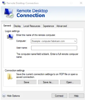
Figure A- 1. Remote Desktop Connection to access TSMA UI... 77

Figure A- 2. WLAN connection between TSMA and laptop ... 77

Figure A- 3. ROMES software icons ... 78

Figure A- 4. StartUp window of ROMES software ... 78

Figure A- 5. User levels ... 79

(12)

XII

Figure A- 7. List of devices connected to TSMA connected to ROMES, Source: [34] ... 80

Figure A- 8. Add/Remove drivers, Source: [34] ... 80

Figure A- 9. Available and loaded drivers (example), Source: [34] ... 81

Figure A- 10. Generated view areas labels... 81

Figure A- 11. RAT selection, Source: [34] ... 82

Figure A- 12. Frequency interval, Source: [34] ... 82

Figure A- 13. Frequency bands available, Source: [34] ... 82

Figure A- 14. ACD view area (before and during measurement) ... 83

Figure A- 15. ROMESMAP Route Track View area (during measurement) ... 83

Figure A- 16. GSM Scanner Top N View during measurement ... 84

Figure A- 17. GSM Scanner Top N Configuration, Source: [34] ... 84

Figure A- 18. GSM Scanner BCH Tree View during measurement ... 85

Figure A- 19. Power Spectrum Overview ... 86

Figure A- 20. Details of the selected sweep ... 86

Figure A- 21. Spectrum History of the selected sweep ... 86

Figure A- 22. Available signals... 86

Figure A- 23. Tools menu ... 87

Figure A- 24. General settings ... 87

Figure A- 25. Performance tab settings ... 88

Figure A- 26. TSMA connections settings ... 88

Figure A- 27. Save workspace file ... 88

Figure A- 28. Start recording button, Source: [34] ... 89

Figure A- 29. Stop button, Source: [34] ... 89

Figure A- 30. Export measurement file to another extension ... 89

Figure A- 31. Export measurement data menu... 90

Figure A- 32. Measurement file to export ... 90

Figure A- 33. Available devices in selected measurement file ... 90

Figure A- 34. ScannerData Export settings ... 91

Figure A- 35. Measurement file (* .rscmd) ... 91

Figure A- 36. Scanner data export result (folder and KML file)... 91

Figure A- 37. Folder content ... 91

TABLE OF TABLES

Table 2- 1. Frequency of the carrier according to region, Source: [9] ... 13

Table 2- 2. Major differences between UMTS and LTE (theoretical), Source: [12] ... 15

Table 3- 1. K value according to d and f units ... 24

Table 3- 2. Parameter values for different types of terrain, Source: [27] ... 32

Table 3- 3. LUI model parameters for three different technologies, Source: [30] ... 34

Table 4-1. Recommended bit rates for video streaming, Source: [31] ... 42

Table 4- 2. RSRP limits for LTE, Source: [35] ... 50

Table 4-3. RSSI limits for GSM/3G(UMTS)/HSPA, Source: [35] ... 50

Table 4-4. Parameter differences between UMTS and LTE ... 52

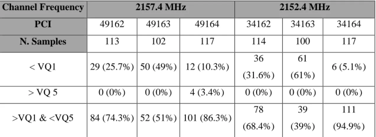
Table 4-5. Nr. of samples and respective percentage for the defined thresholds ... 54

Table 4-6. Main parameters for all sectors in reference BS ... 55

(13)

XIII

Table 4-9. Main parameters for all sectors in reference BS ... 60

Table 4- 11. Main parameters for all sectors in reference BS ... 62

Table 4- 14. Nr. of samples and respective percentage for the defined thresholds ... 66

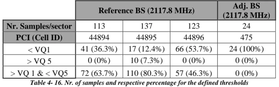
Table 4- 16. Nr. of samples and respective percentage for the defined thresholds ... 69

Table 4- 17. Main parameters for all the cells from reference BS ... 70

TABLE OF GRAPHICS

Graphic 3 - 1. "Below BS antenna difference using 𝝌𝒂𝒏𝒈𝒍𝒆𝒔 ", Source: [1] ... 38

Graphic B - 1. All sectors/cells from reference BS (eNodeB: 1675) ... 94

Graphic B - 2. Reference sector below the highest quality threshold ... 94

Graphic B - 3. Throughput vs RSRP from the reference sector ... 94

Graphic B - 4. Order 2 polynomial trendlines for every sector in reference BS ... 95

Graphic B - 5. RSRP vs Height vs Distance to BS (PCI_177) ... 95

Graphic B - 8. Throughput vs Time [All sectors, reference BS] ... 96

Graphic B - 9. Reference sector throughput below minimum threshold ... 96

Graphic B - 10. Throughput vs RSSI [reference sector] ... 97

Graphic B - 11. Order 2 polynomial trendlines for every cell in reference BS ... 97

Graphic B - 12. Throughput vs Time [All sectors, reference BS] ... 97

Graphic B - 13. Signal strength from reference sector below minimum threshold ... 98

Graphic B - 14. Order 2 polynomial trendlines for every cell in reference BS ... 98

Graphic B - 15. RSSI vs Height vs Distance to BS (Reference cell: 34164) ... 98

Graphic B - 16. RSSI vs Height vs Distance to BS (Cell 34163) ... 99

Graphic B - 17. RSSI vs Height vs Distance to BS (Cell 34162) ... 99

Graphic B - 18. Throughput vs Time considering all sectors from reference BS ... 99

Graphic B - 19. Reference sector results below VQ5 threshold ... 100

Graphic B - 20. Throughput vs RSRP for all sectors from reference BS ... 100

Graphic B - 21. RSRP vs Height vs Distance to BTS for sector 177 (adjacent) ... 100

Graphic B - 23. RSRP vs Height vs Distance to BTS for sector 178 (reference) ... 101

Graphic B - 24. Throughput vs Time for all sectors from the reference BS ... 101

Graphic B - 25. Reference sector throughput below poorest quality threshold ... 102

Graphic B - 29. Throughput vs Time considering all the cells from the reference BS ... 103

Graphic B - 30. Reference sector throughput below the HQ threshold ... 104

Graphic B - 31. Throughput vs RSRP for reference eNodeB/BS ... 104

Graphic B - 35. Throughput vs Time considering sector from adjacent BS ... 105

(14)

XIV

Graphic B - 37. Reference sector below minimum VQ threshold ... 106

Graphic B - 38. Throughput vs RSSI for every sector in reference BS ... 106

Graphic C - 1. PDF of RSRP; LTE: 796 MHz; Sc: A ... 109

Graphic C - 2. CDF of RSRP; LTE: 796 MHz; Sc: A ... 111

Graphic C - 3. CDF of Throughput; LTE: 796 MHz; Sc: A ... 112

Graphic C - 4. PDF of Throughput; LTE: 796 MHz; Sc: A ... 113

Graphic C - 5. CDF of RSSI; UMTS: 2152.4 MHz; Sc: A ... 113

Graphic C - 6. PDF of RSSI; UMTS: 2152.4 MHz; Sc: A ... 115

Graphic C - 7. CDF of Throughput; UMTS: 2152.4 MHz; Sc: A ... 116

Graphic C - 8. PDF of Throughput; UMTS: 2152.4 MHz; Sc: A ... 116

Graphic C - 9. CDF of RSRP, LTE: 796 MHz; Sc: B ... 117

Graphic C - 10. PDF of RSRP, LTE: 796 MHz; Sc: B ... 117

Graphic C - 11. CDF of Throughput; LTE: 796 MHz; Sc: B ... 119

Graphic C - 12. PDF of Throughput; LTE: 796 MHz; Sc: B ... 119

Graphic C - 13. CDF of RSSI; UMTS: 2152.4 MHz; Sc: B ... 120

Graphic C - 14. PDF of RSSI; UMTS: 2152.4 MHz; Sc: B ... 121

Graphic C - 15. CDF of Throughput; UMTS: 2152.4 MHz; Sc: B ... 121

Graphic C - 16. PDF of Throughput; UMTS: 2152.4 MHz; Sc: B ... 122

Graphic C - 17. CDF of RSRP; LTE: 806 MHz; Sc: C ... 123

Graphic C - 18. PDF of RSRP; LTE: 806 MHz; Sc: C ... 124

Graphic C - 19. CDF of Throughput; LTE: 806 MHz; Sc: C... 125

Graphic C - 20. PDF of Throughput; LTE: 806 MHz; Sc: C ... 125

Graphic C - 21. CDF of RSSI; UMTS: 2117.8 MHz; Sc: C ... 126

Graphic C - 22. PDF of RSSI; UMTS: 2117.8 MHz; Sc: C ... 127

Graphic C - 23. CDF of Throughput; UMTS: 2117.8 MHz; Sc: C ... 127

(15)

XV

SYMBOLS

𝒉𝒓 Receiver antenna height

𝒉𝒕 Transmitter antenna height

𝑪_𝑯 Antenna height correction factor

𝑳𝟎 Free space propagation loss, which comes from FSPL formula

𝑳𝑳𝑶𝑺 Path loss in Line of Sight situation (Walfish-Ikegami)

𝑳_{𝑵𝑳𝑶𝑺} Path loss in Non-Line of Sight situation (Walfish-Ikegami) 𝑳𝑶 Path loss considering an open area

𝑳_𝑼 Path loss result for small city considering urban environment equation 𝒅_𝒃𝒑 Breakpoint distance

𝒌_𝑻𝑬𝑪 Constant that assumes a different value according to the size of the cell 𝝌𝒂𝒏𝒈𝒍𝒆𝒔 Correction factor that use several parameters related to the antennas

𝝌𝜽+𝝍 Correction factor considering the elevation and the tilt of the antenna

𝝌𝝋+𝜷 Correction factor that considers azimuth (𝜑) and 𝛽

AMU (f,d) Median attenuation related to free space d Distance between transmitter and receiver

d0 Reference distance that vary according to the technology in use f Frequency of signal transmission

G(hr) Mobile antenna height gain factor (receiver)

G(ht) BS antenna height gain factor (transmitter)

Garea Gain depending on the type of environment/terrain

Lmsd Multiscreen diffraction related to urban rows of buildings

Lrts Correction factor related to diffraction and scattering from rooftop to street

𝚫𝑳𝒃,𝒇 Frequency correction factor (Basic SUI Model)

𝚫𝑳𝒃𝒉 Receiver/terminal antenna height correction factor

𝑩 Channel Bandwidth

𝑪 Channel Capacity/Throughput

𝑳 Median value of propagation path loss

𝒂(𝒉_𝑹) UE antenna height correction factor as described in the Hata Model for urban areas

𝒄 Speed of light in vacuum (~ 3 × 108_{[m/s] )}

(16)

XVI 𝜸 Path loss exponent

𝜽 Elevation angle

𝝋 Azimuth

(17)

XVII

ACRONYMS & ABBREVIATIONS

2D Two coordinates system (two dimensions)

3D Three coordinates system (three dimensions)

3G Third Generation technologies

3GPP Third Generation Partnership Project (3GPP)

4G Fourth Generation technologies

AuC Authentication Center

BS Base Station

BSC Base Station Controller

BSS Base Station Subsystem

BTS Base Transceiver Station

CI Cell Identity

CDF Cumulative Density Function

CN Core Network

DCS Digital Cellular System

DD Digital Dividend

DDF Dirac Delta Function

DL DC Downlink Dual Carrier

EDGE Enhanced Data rates for Global Evolution

FDD Frequency Division Duplex

GPS Global Positioning System

GSM Global System for Mobile Communications

HLR Home Location Register

HSPA High Speed Packet Access

IN Intelligent Network

LAC Location Area Code

LoS Line of Sight

LTE Long Term Evolution

LUI Lisbon University Institute

MCC Mobile Country Code

MNC Mobile Network Code

(18)

XVIII

NLoS No line of sight

NSS Network subsystem

OFDMA Orthogonal Frequency-Division Multiple Access

OS Operating System

PAPR Peak to Average Power Ratio

PC Personal Computer

PCI Physical Cell Identity

PDF Probability Density Function

QoE Quality of Experience

QoS Quality of Service

RC Radio Communications

RF Radio Frequency

RNC Radio Network Controller

RSCP Received Signal Code Power

RSRP Reference Signal Received Power

RSRQ Reference Signal Received Quality

RSSI Received Signal Strength Indication

SC Satellite Communication

SC-FDMA Single-Carrier Frequency-Division Multiple Access

SINR Signal to Interference Plus Noise Ratio

SMS Short Message Service

SNR Signal to Noise Ratio

SUI Stanford University Interim

TDD Time Division Duplex

UAV Unmanned Air Vehicles

UE User Equipment

UMTS Universal Mobile Telecommunications System

UTC Universal Time Coordinated

UTRAN UMTS Terrestrial Radio Access Network

VLR Visitor Location Register

VQ Video Quality

WCDMA Wide Band Code Division Multiple Access

(19)

1

CHAPTER 1

INTRODUCTION

Overview, motivation, objectives, contributions and dissertation structure are available in this chapter

(20)

2

1.1 Overview

Ten years ago, it was unthinkable that UAVs could reach such success in civil and even in commercial industries. Nowadays, it is mandatory to think that not only smartphones or laptops can depend on cellular mobile networks, but also these vehicles. However, the existent propagation models do not yet consider this possibility, which is why it is so important to create or redefine some of these models to establish a solution since the UAV’s market is growing exponentially, justified by the large amount of applications related to it.

Actually, most of these UAVs establish a connection to the user provided by radio communication (RC) but it is not reliable when there is no line of sight (LoS) between the two intervenient. However, it is possible to establish a link between both but only by using satellite communication (SC) that is extremely expensive and only reachable for military purposes. To overtake this problem, cellular mobile networks are an alternative to RC and SC, where the LoS and high costs will no longer be an obstacle.

The cellular mobile networks considered use UMTS and LTE technologies since they are capable to reach faster data rates and permit lower latency, which is extremely important when applications like streaming is used, since it requires large sets of data in a short period.

One of the main focus of this thesis considers the “hole phenomenon” that occurs above the antennas where the radiation pattern is not reachable. Considering this, it is important to examine the signal strength based on measurement campaigns since it’s a crucial parameter to confirm if in a problematic situation (e.g., weak signal strength) it’s still possible to maintain vital services for a specific application (e.g., video streaming) appealing to handover, or if it’s not even necessary to consider this option. It is also mandatory to verify if the service provider infrastructure is prepared to solve this problem by establishing communication with another base station (handover) whenever it is necessary to keep providing a good signal strength to maintain an acceptable QoS when considering video streaming application.

It is possible to maintain acceptable signal strength values for video streaming application when considering an outdoor scenario and variations in 2D coordinates (e.g., altitude or distance vs signal strength) [1]. One of the challenges proposed in this reference was to study the signal’s propagation when the variation between two crucial parameters occur

(21)

3 simultaneously (distance and altitude) in suburban and rural scenarios. In this dissertation, only rural scenarios are considered.

Besides that, it is necessary to examine a propagation model that fits the UAV’s demands, its own characteristics and capabilities since these are different from the usual UEs. Lisbon University Model (LUI Model) is a possibility because it is able to support UMTS and LTE when considering correction factors and the use of experimental results [2].

1.2 Motivation

Drones have a fundamental role in society based on its increasing impact in the most diverse areas. About ninety percent (90%) of the investment made in this market was only for military purposes [3], but this number tends to decrease in medium/long term since these vehicles are already in use for civil and industrial purposes with several interesting applications, whose description is below:

- Inspection and monitoring:

o Inspection of oil and gas platforms;

o Inspection of infrastructures like bridges, roads, railways, etc.; o Preventive action or emergency cases.

- Surveying and mapping:

o Land cover classification and mapping;

o Surveying and mapping for cartography, topography, cadastral surveys and urban and regional development;

o Archeological surveys and excavation monitoring. - Precision agriculture:

o Ecological and agronomic rural cultivation; o Analysis of soil, health and vigor of crops. - Condition Survey and Civil Engineering;

- Aerial Imaging – HR Photos; - HD Film and Video.

Based on all the applications mentioned above, a well-implemented network infrastructure is crucial to guarantee a stable communication between the user and the drone. To guarantee a reliable connection, the signal’s propagation conditions and the adequate propagation model are crucial parameters of analysis. To choose a certain model, several aspects are studied:

(22)

4 - Scenarios:

o Rural, suburban or urban o Outdoor or indoor - Frequency range;

- Antenna description and its characteristics: bandwidth, gain, polarization, (ir)radiation pattern, physical (e.g., transmitter/receiver antenna height) and mechanical characteristics.

1.3. Objectives

Considering the cellular networks potential for UAVs communication environment, it is important to upgrade or develop a new propagation model that considers all the factors that might affect the link between the controller and the vehicle by providing a good QoS in video streaming service. UMTS and LTE are the main technologies since these are capable to provide higher data rates, which are fundamental to this function. LUI is an empirical propagation model, which main concern is the urban scenario but only considering 2D and not 3D coordinates, which is necessary in this dissertation. Having this, it is mandatory to study all the scenarios using three dimensions, in order to achieve a sustainable and reliable propagation model proposal.

Besides that, the hole phenomenon over the antennas is also considered to conclude if we can still maintain a good signal strength, since theoretically this parameter values drop dramatically and might not guarantee an acceptable quality of service depending on the application. If that happens, it is possible to answer if the actual infrastructure for a specific service provider (e.g., NOS, Vodafone and MEO) in a certain environment and location is prepared to support this event or not.

It is possible to synthetize all this information in five topics:

1. Analyze the equipment and conclude which one meets the measurement campaigns requirements;

2. Measurement campaigns in a specific scenario (outdoor and rural) using the equipment attached to the UAV and considering a specific and controlled flight route;

3. Filter all the information provided by the instrument by studying how signal propagation behaves along the flight considering fundamental parameters (e.g., signal strength, quality, etc.), which might lead to several conclusions:

(23)

5 a. Is it possible to maintain a good QoS for video streaming in every single

coordinate of UAV’s flight?

b. Is the actual infrastructure from a specific service provider prepared to handle handover considering UAVs characteristics (e.g., height, distance, etc.)?

4. Propose or sustain an existent propagation model (e.g. LUI model) that considers UAVs unique characteristics when compared with general UEs (e.g. smartphone, laptop, etc.), which are considered by other models (e.g. Okumura);

5. Comparison between theoretical and empirical approaches about the “hole phenomenon”.

1.4. Contributions

This dissertation proposes to develop or sustain empirically an already existent propagation model considering cellular networks (UMTS and LTE technologies) in a 3D coordinates system where the drone changes its distance and altitude simultaneously during its flight route. Besides that, it also analyzes the capacity of a specific service provider infrastructure to handle a handover event, if necessary. For example, if the antennas from the reference BTS cannot provide enough conditions to handle video streaming in a specific quality and there’s a great possibility that this might happen when “hole phenomenon” occurs (theoretically), it has to exist another adjacent BTS that is able to compensate the lack of signal conditions from the previous one and maintain an acceptable QoS.

A full paper named “Cellular networks capacity to support video broadcasting in UAVs communications environments” has been submitted to IEEE VNC 2017 conference relying on the thesis developments.

1.5. Dissertation Structure

This section presents the dissertation structure, which is divided into 5 chapters:

 Chapter 1 presents the overview, motivation, the objectives for this dissertation and respective contributions.

 Chapter 2 describes the general concepts about 2G, 3G and 4G technologies used in current cellular network infrastructures, the related events that might occur during the mobile station use and the frequency bands for each in technology in

(24)

6 Portugal. Besides that, it also studies the physical equipment like the drone in use and its definition and also the available spectrum analyzers by comparing them and define which one is the most reliable for measurements in unique conditions.  Chapter 3 presents the characteristics of the most used propagation models for

outdoor scenarios in current cellular networks and studies whether any of the available ones is able to support the characteristics of a drone or if it requires an extension of the previous models or the development of a new one model.

 Chapter 4 reveals the measurement results for three different locations by using 2D and 3D graphs to study the “hole phenomenon” relying on several parameters provided by the spectrum analyzer.

 Chapter 5 shows the main conclusions of all the work done in this thesis and shares some proposals to take into account for a future project.

(25)

7

CHAPTER 2

CONCEPTS

This chapter provides crucial concepts that are (in)directly related to this dissertation’s main objectives, such as UMTS, LTE technologies and handover phenomenon. UAV and equipment requisites for measurement campaigns are also considered.

(26)

8

2.1 Cellular Networks

The cellular network infrastructure bases on cells/sectors, which distribution is according to land areas served by at least one base station. Considering this, it is possible to provide network coverage to the cell that require voice and data traffic used in various applications. To avoid interference and maintain an acceptable QoS, each cell uses a different set of frequencies.

Considering that only base station will not provide enough radio coverage for a wide geographic area, it is necessary to join various cells from different base stations, in order to communicate between a large number of users in different locations using the same network. The fact that users might be moving from cell to cell (e.g., walk/car travel) is contemplated and it is called handover phenomenon.

There are several recognizable aspects in cellular networks:

- Capacity: capable to have more capacity considering the fact that uses more than a single transmitter, since the same frequency might be enable for multiple links as long as they are in different cells;

- Power: with the large quantity of base stations that exist, it is possible to conclude that the distance between these and the user is not as big as if only single large transmitter is used. Considering this, it is possible to achieve that mobile devices use less power because they are closer to the cell towers due to their quantity;

- Coverage: when compared to a single terrestrial transmitter, this parameter can be improved anytime since additional cell towers can be added indefinitely and are not limited by the horizon.

Mobile phone service carriers (e.g., Vodafone, MEO) provide these networks and each one has their own carriers. The user might pick up a cell signal provided by one of the mentioned carriers, but the signal’s strength might be different in distinct locations since it depends on the carriers’ licenses that define the technology in use on each cell. In

(27)

9 Portugal, 3G and 4G are dominant in metropolitan areas. In less populated areas, the signal might assume worst rates (e.g., GSM, EDGE) or, in the worst case, no coverage.

Figure 2- 1. Cellular Networks technologies evolution, Source: [4]

Nowadays, almost everyone owns a smartphone and there is an extreme necessity to send and receive large amounts of data in a short period, which relate to the content traded between users. Assuming that most of the content requires big data rates for photos, videos and streaming applications, this can only be provided when using the most advanced technologies, and that is the main reason why is so important to analyze people’s tendencies and the respective evolution of cellular networks throughout the time.

2.1.1 GSM

Global System for Mobile Communications or GSM has become the dominant 2G radio access standard since its introduction, in the early 1990s. However, it still is widely used all over the world and there were about 3 million subscribers in 2010. Its growth has taken place with the large experienced expansion of access to the Internet, multimedia services. In addition, improvement in transmission quality, system capacity, coverage and standardization.

Speech transmission prevails to be dominant when compared to 1G, but services like SMS or fax emerged with it, by accomplishing higher demands. Regular improvements in all areas of telecommunication technology and the resulting steady price reductions for both infrastructure equipment and mobile devices were fundamental parameters to achieve it. Despite its age and the evolution toward new technologies (e.g., UMTS and LTE), GSM continues to be developed and has been enhanced with many features in recent years in

(28)

10 order to introduce new functionality and decrease operational cost to the service providers.

Figure 2- 2. GSM Coverage Worldwide, Source: [5]

A network based in GSM technology uses three subsystems [6]:

 Base Station Subsystem or BSS is the radio network and it is responsible to provide wireless connection to mobile subscribers over the radio or air interface by using all given nodes and functionalities from this subsystem.

 Network Subsystem or NSS is the core network, it contains all nodes, and functionalities that are fundamental for services like call switching, subscriber and mobility management.

 Intelligent Network Subsystem or IN can trigger optional functionalities to the network. This subsystem allows subscribers to first fund an account with a certain amount of money, which can be used later in network services like SMS, phone calls, etc. As an example, an IN node is contacted and the network operator (e.g., NOS) will deduct from a prepaid subscriber account in real time if the subscribers uses a service.

(29)

11

Figure 2- 3. GSM Architecture, Source: [6]

Some of the definitions from the previous illustration are available below:

 BTS – Base Transceiver Station – provides the communication between user equipment and the network. It is commonly composed by: transceiver, power amplifier, antenna, etc.

 BSC – Base Station Controller – establishment, release and maintenance of all connections of cells that are connected to a base station.

 MSC – Mobile Switching Center – connections between subscribers’ management;

 VLR – Visitor Location Register – signaling reduction between the MSC and the HLR;

 HLR – Home Location Register – subscriber DB of a GSM network that stores information about the individually available services;

 AuC – Authentication Center – contains an individual key per subscriber which is a copy of the same key on the subscriber’s SIM card. It is where the authentication process performs (e.g., establishment of a call and guarantees that the subscriber’s id is not misused).

However, GSM was not able to meet the users’ demands for better and faster data communications, which makes network and service evolution necessary in order to accomplish end users demands throughout time. EDGE (pre-3G) emerged in order to accomplish higher data rates and was able to accomplish several tasks like reduced latency, increased peak bit rate up to 1 Mbit/s by using DL DC and higher order modulations (16 and 32-QAM). Nonetheless, the 2G technologies were unable to meet the growing demand for more network capacity and 3G emerge to overtake this barrier.

(30)

12

2.1.2 UMTS

Universal Mobile Telecommunications System or UMTS is part of the third generation (3G) family, where mobile systems had the possibility to evolve and define new services like e-mail, mobile internet browsing, high speed data transfer, audio streaming (e.g., Spotify), multimedia, etc. When analyzing the previous examples, it is noticeable that UMTS network relates to data services that require newer QoS requirements, different traffic characteristics and updated bandwidth when compared to older technologies [7]. Several challenges were taking into account to develop this technology:

- Redesign the existing cellular technology to maximize the spectrum efficiency for voice and data services because GSM mainly goal was to provide high-quality voice services;

- Provide global roaming and interoperability of different mobile communications across diverse mobile environment.

Its architecture is composed in three domains: radio access network or UTRAN (Universal Terrestrial Radio Access), a core network (CN) based on the GSM Phase 2+ and the UE (e.g., smartphones, laptops, etc.).

UTRAN functionalities relate to resource management, admission control functionality and sets up the bearers enabling the user equipment to communicate with the core network.

CN manages telecommunication services for each UMTS subscriber. These services might relate to mechanisms for UE authentication, users’ charging, etc.

(31)

13 In the same architecture, Uu and Iu stand for standardized interfaces that enable the communication between the three previous domains and also permit a UMTS operator to select different equipment suppliers for each domain.

The first release about UMTS was in March 2000 (Release 99), where it describes that two W-CDMA modes co-exist in UTRAN:

- FDD – Frequency Division Duplex – two different frequency bands are used for the uplink and downlink directions and the frequency separation between both might assume 190 MHz or 80 MHz;

- TDD – Time Division Duplex – Same frequency used for both the uplink and downlink allowing asymmetric traffic in both directions depending on the number of timeslots configured for each link.

Table 2- 1. Frequency of the carrier according to region, Source: [9]

Besides WCDMA, 3GPP developed other technologies in 3G era. HSPA and HSPA+ are already considered as 3.5G and were the latest before 4G emerge, being able to reach a downlink data speed of 7.2 Mbit/s and 21.6 Mbit/s, respectively, against the 384 kbit/s provided by WCDMA [10]. These values are theoretical and defined by the available network service providers (e.g., NOS).

Considering the previous information, UMTS includes W-CDMA scheme using paired or unpaired 5 MHz wide channels and able to use two modes: TDD and FDD. However, downlink speed might be a limitation when comparing to HSPA and HSPA+ that are able to give greater bit rates and improves packet-switched applications [9].

2.1.3 LTE

Long Term Evolution emerges with the need to enhance and accomplish the following tasks [11]:

(32)

14 - Higher capacity/spectral efficiency (e.g., end-users might be affected when

capacity shortage occur); - Cost reduction;

- Low complexity;

- Packet switch optimized system; - Low delay;

- Frequency and bandwidth are not constant and might vary.

Figure 2- 5. Network infrastructure from GSM to LTE, Source: [11]

The LTE access network uses base stations denominated as eNodeB (eNB). This network uses a flat architecture where the intelligence distribution is amongst the base stations to ensure a higher speed set-up, fast communication and decisions between the eNB and the UE, and reduce delay for handover process. This process is essential when an end-user is using a real-time service that require high data peak rates (e.g., video streaming, online gaming, etc.).

LTE uses OFDMA for the downlink and SC-FDMA for the uplink, in order to achieve high radio spectral efficiency and enable efficient scheduling and frequency domain.

Figure 2- 6. OFDMA (DL) and SC-FDMA (UL), Source: [11]

OFDMA and SC-FDMA are modulation techniques. OFDM or Orthogonal Frequency Division Multiplexing encodes digital data in subcarriers from the available bandwidth. Orthogonal Frequency Division Multiple Access or OFDMA use these subcarriers and

(33)

15 share them between multiple users leading to high peak to average power ratio (PAPR) that increases the power consumption for the sender caused by power amplifiers.

SC-FDMA is the second modulation technique and creates a signal with single carrier characteristics, but the power consumption is lower when compared with OFDMA. In order to support as many requirements as possible, LTE uses:

- E-UTRA operating bands from 700 MHz to 2.7 GHz; - Channel bandwidths: 1.4, 3, 5, 10, 15, or 20 MHz - Support two sub-modes: TDD and FDD

- In Release 8 from 3GPP, 8 bands specified for TDD mode were available; - In Release 9 from 3GPP, 19 bands specified for FDD mode were available.

Table 2- 2. Major differences between UMTS and LTE (theoretical), Source: [12]

Analyzing the previous table, the differences between UMTS and LTE over similar parameters are notorious. LTE network is clearly superior when considering high data rate services, which makes it capable to accomplish end-users demands and achieve new stablished QoS requirements (theoretically).

2.1.3 Handover

Handover is the most important process because it provides mobility in cellular architectures and can accomplish user preferences. It enables continuity of mobile services to an end-user when in an ongoing communication and crossing the cell edge. Per example, when the end-user is at the cell edge, the signal strength provided from the

(34)

16 current cell might drop below a defined threshold value, making it worse when compared to another cell that can provide more favorable radio resources. Every time this situation occurs, there is a need for handover in order to maintain a good QoS.

The whole process of disconnecting from the current cell and establish a new connection in the proper cell is the handover process and it is equally important in voice services and data services.

There is more than one type of handover and this process might differ from technology to technology. In W-CDMA, there are three types of handover: hard, soft and softer handover.

 Hard handover uses the same process used for 2G networks where the radio links are broken and then re-established. In this process, user might notice a break in the connection and it might fail when re-establishing the link between the user and the new NodeB.

Figure 2- 7. Hard Handover, Source: [13]

RNC stands for Radio Network Controller (figure 2-7) and its main responsibility is to control the NodeBs connected to it, being also able to manage radio resources and mobility functions.

 Soft handover occurs when the UE is in the overlapping coverage area of two cells. The cell phone or UE is able to establish links with more than one base station simultaneously but these BSs have to be operating on the same frequency or channel. Having this, it will provide a more reliable way to perform handover.

(35)

17

Figure 2- 8.Soft Handover, Source: [13]

 Softer handover is similar to soft handover, but in this case, UE establishes new radio links served from the same base station or NodeB.

Figure 2- 9. Softer Handover, Source: [13]

Briefly, UMTS handover methodology evaluates information about the signals received by UE and the base station, considering parameters like RSCP and RSSI. When these parameters decrease significantly, assume values below a defined threshold and there is another available radio channel, which is able to improve radio resources, it triggers handover process [14].

There are also three types of handover in LTE network: Intra-LTE Handover, Inter-LTE Handover and Inter-RAT.

 Inter-LTE/Inter-RAT handover - the UE leaves an eNodeB sector to a sector controlled by an adjacent or neighbor eNodeB.

(36)

18

Figure 2- 10. Inter-LTE/RAT Handover, Source: [15]

 Intra-LTE handover - UE moves from one sector to another sector and both sectors belong to the same eNodeB.

Figure 2- 11. Intra-LTE Handover, Source: [15]

2.2. Drone

Drones can fly autonomously using onboard computers, but also under remote control by a human operator where RC is the most common type of communication established between the controller and the vehicle, but it is not efficient when there is no line of sight. Cellular networks might be effective in both cases mentioned above, because the distance between the intervenient could be larger and the user controlling it could see what the drone is filming by using video streaming application supported by these networks. Considering this, it is crucial to verify the reliability and capacity of the actual infrastructure by using a real-life drone to simulate several flight routes attaching the spectrum analyzer to the UAV that will receive essential parameters based on UMTS and LTE technologies and will lead us to answer wetter video streaming is possible and in what conditions.

(37)

19

Figure 2- 12.Octocopter (drone) with TSMA attached (under it)

In this case, only an UAV that lifts the spectrum analyzer’s weight (~2.5 kg) is able to do measurement campaign. However, in order to simulate a real-life scenario, the octocopter represented in the figure 2-12 is used.

2.3. Spectrum Analyzer

The analysis of the possible spectrum analyzers is required before concluding which one would accomplish this dissertation’s challenges/requisites in measurement campaigns:

1) Spectran HF-60100 is a measurement device that uses a frequency dependent measurement approach, the so-called spectrum analysis. It determines the signal strength for every individual signal in a certain frequency range defined by the user. However, the battery does not last long (~20 minutes), the memory size is limited in autonomous mode and the output parameters are not enough to obtain a sustainable conclusion.

Figure 2- 13. Spectran HF-60100, Source: [16]

2) R&S TSME is a scanner that measures up to eight different technologies simultaneously in the 350 MHz to 4.4 GHz. It is compact, lightweight, low power consumption and it has an internal GPS. Besides that, it also provides information related to base station ID, signal strength/quality, SINR and several codes (MCC

(38)

20 and MNC) that will permit to identify the service providers. The only defect is that needs a full-time connection to a host PC [17].

Figure 2- 14. R&S TSME scanner connected to a PC, Source: [18]

3) R&S TSMA is similar to TSME but the main difference between the two is that TSMA is battery powered with rechargeable batteries and charging function, ensuring that is always ready to operate. It delivers all measurement results required for optimizing LTE networks. These include power and quality measurements (RSRP, RSRQ, SINR) on reference signals for all eNodeBs transmission ports. Having this, it’ll be possible to analyze and detect radio dead zones (e.g., “hole phenomenon”) or locations with too much interference. TSMA already comes with ROMES software, where it is possible to analyze the signal’s behavior while the instrument is capturing it from several base stations that use different technologies (e.g., GSM, UMTS, and LTE) and/or save it in measurement files for posterior analysis [19].

The only requirement to access Windows OS in TSMA is a monitor or a tablet/smartphone/laptop connected to it using WLAN or Bluetooth to provide a user interface for previous configuration before starting the measurement campaign and for posterior analysis when access to measurement files is required. In this case, the only defect is the weight (~ 2.5 kg) but it is possible to overcome this problem by using a medium/heavy weight drone (e.g., octocopter).

(39)

21

Figure 2- 15. R&S TSMA scanner and TSMA-BP (battery pack), Source: [20]

After evaluating these three analyzers, it is clear that R&S TSMA Scanner together with a battery pack is the first choice because it accomplishes the most important challenges when compared to the others: battery autonomy and independency.

2.4. Frequency bands

This section pretends to share the frequency bands in use in Portugal territory for GSM, UMTS and LTE networks. The well-known network service providers in Portugal: MEO, NOS and Vodafone, use most of the bellow frequency bands [21].

 GSM: o E-GSM (900 MHz) o DCS (1800 MHz)  UMTS: o B1 (2100 MHz) o B8 (900 MHz)  LTE: o B3 (1800 +) o B7 (2600 MHz) o B20 (800 DD)

(40)

22

CHAPTER 3

PROPAGATION

MODELS AND

PROPOSED MODEL

This chapter describes the most used propagation models in actual cellular networks and proposes a new model or support empirically to an already existent one.

(41)

23

3.1. Overview

Propagation models are able to provide an attenuation estimation based on the transmitted signal that previews its behavior for different types of scenario. Nonetheless, there are three types of propagations models: empirical, theoretical and hybrid [22]. The characteristics for each different model are below:

 Empirical model:

o Considers measurement data;

o Simple relation between attenuation and distance

o Ponder all the factors that affect the signal’s propagation; o Consider a specific scenario to study this model.

 Theoretical model:

o Uses topographic databases;

o Counts some factors that might affect the signal’s propagation but not all; o The scenario is irrelevant.

At last, hybrid models conjugate both empirical and theoretical models and it is able to reduce the error percentage by considering the relation between the estimated and the measured signal, which makes it more accurate.

This project bases on measurement campaigns, which coincides with the empirical model characteristics. Considering this, it is important to evaluate the already existing propagation models in order to reduce the number of possibilities and verify which adapts to the thesis requirements (e.g., scenarios, UAVs characteristics, technologies, etc.).

3.2. Propagation models

This section provides information about the existent propagation models for outdoor environments and it synthesizes the characteristics of each.

3.2.1. Okumura Model

Okumura model is one of the most known models in use for signal prediction and its impact area is mainly in cities. However, its structure bases in three modes: urban, suburban and open areas [23].

(42)

24 This model’s mathematical formulation is:

𝐿 [dB] = 𝐿0 [dB] + 𝐴𝑀𝑈[dB] − 𝐺(ℎ𝑡) − 𝐺(ℎ𝑟) − 𝐺𝑎𝑟𝑒𝑎 (3.1)

The equation (3.1) depends on several parameters, which explanation is as it follows:  L [dB] – median value of propagation path loss;

 𝐿₀ [dB] – free space propagation loss, which comes from FSPL formula calculation;

 AMU (f,d) [dB] – median attenuation related to free space;

 G(ht) - BS antenna height gain factor (transmitter);

 G(hr) - mobile antenna height gain factor (receiver);

 Garea – gain depending on the type of environment/terrain.

In order to get a result from the previous formula, it is important to calculate FSPL in decibels (dB): 𝐹𝑆𝑃𝐿 _{𝑙𝑖𝑛𝑒𝑎𝑟} = (4𝜋𝑑𝑓 𝑐 ) 2 (3.2) 𝐹𝑆𝑃𝐿_[dB] 𝑜𝑟 𝐿0[dB] = 20𝑙𝑜𝑔10(𝑑) + 20𝑙𝑜𝑔10(𝑓) + 𝐾 (3.3)

Based on the two preceding formulas, c stands for speed of light in vacuum (~ 3 × 108_{[𝑚/𝑠] ), d is the distance between the transmitter and receiver, f is the signal}

frequency and K is a constant that can assume more than one value since it depends on the previous parameters units and the following table is able to explain it:

K value Distance units Frequency units

92.45 Kilometers [km] Gigahertz [GHz]

-87.55 Meters [m] Kilohertz [KHz]

-27.55 Meters [m] Megahertz [MHz]

32.45 Kilometers [km] Megahertz [MHz]

Table 3- 1. K value according to d and f units

Amu (f,d) result is also required but it depends on the reference height of the base station

and mobile antennas, which are 200 m and 3 m, respectively. If the real heights from the transmitter and receiver antennas or if the propagation type differ from the reference results, corrections implementation are mandatory. However, the following illustration

(43)

25 shows the results for the reference heights in an urban environment over a quasi-smooth terrain.

Figure 3- 1 - Median attenuation related to free space (Okumura model), Source: [23]

The gains from the transmitter (Ght) and receiver (Ghr) antennas are also mandatory:

𝐺(ℎ_𝑡) = 20 log (ℎ𝑡

200) 30 m < ℎ𝑡 < 1000 m (3.4)

The value “200” present in the only fraction from the previous formula stands for the base station antennas reference height. However, this formula is only useful if the transmitter antennas do assume heights between 30 and 1000 m. The following figure illustrates the gain’s behavior considering that interval.

(44)

26 Unlike the previous situation, Ghr depends on the mobile’s height and uses two formulas.

However, the results might vary according to the operating frequency, which is more noticeable when the mobile is closer to upper limit height (~ 10 meters).

𝐺(ℎ_𝑟) = 10 log (ℎ𝑟

3), ℎ𝑟 ≤ 3 m (3.5)

𝐺(ℎ_𝑟) = 20 log (ℎ𝑟

3), 3 m < ℎ𝑟 < 10 m (3.6)

Figure 3- 3. Mobile height gain factor, Source: [23]

It is possible to conclude that mobile antennas that assume heights below 3 meters cause loss of referent signal level. When at 3 meters height, the gain is null. However, from 3 to 10 meters height, the antennas introduce gain that tend to increase while increasing the altitude, until it reaches its maximum gain at 10 meters height, which is the maximum limit for this model.

At last, Garea is the only parameter missing to calculate the median value of propagation

path loss, which stands for correction factor and varies according to the type of environment, as it is possible to realize from the following illustration:

(45)

27

Figure 3- 4. Correction factor for different types of terrain, Source: [23]

In this case, different types of terrain assume distinct gain values that also vary according to the operating frequency. Open area environment is the only one that coincides with the proposed scenarios in this dissertation.

In the end, it is possible to summarize this propagation model considering the following characteristics:

 Frequency f : (150-1920) [MHz] but can extrapolate up to 3000 MHz  Distance d: (1 – 100) [Km]

 BS antenna height (he): (30 – 1000) [m]

 UE antenna height (hr): (1 – 10) [m]

The main technique to determine the path loss follows three steps:

1. Determine free space path loss between the transmitter and the receiver;

2. Read the value Amu (f,d) from the curves in the graphic represented in figure 12

and also consider correction factors related to the type of terrain;

3. The remaining graphics are able to provide the gain values: Gt, Gr and Garea;

This propagation model does not fit in the scenarios considered in this dissertation measurement campaigns because the UE height maximum limit in this model is not high enough when comparing to the heights that UAV might assume (~ 60 meters).

(46)

28

3.2.2. Hata Model

Hata or Okumura-Hata model interprets graphical information from Okumura model, but it considers effects like diffraction, reflection, and scattering caused by cities structures (e.g., buildings, streets, etc.). Besides that, it also improves urban, suburban and rural scenarios with the corresponding corrections. However, characteristics as frequency interval, base station height, link distances and the corresponding formula are different. Hata model considers the following characteristics:

 Frequency f : (150-1500) [MHz]  Distance d: (1 – 10) [km]

 BS antenna height (he): (30 – 200) [m]

 UE antenna height (hr): (1 – 10) [m]

Each scenario has a specific set of equations, but considering the place where the measurement campaigns take place, it is important to give most attention to rural. This environment is comparable to an open area where there are no obstacles to affect the signal transmission.

𝐿𝑂[dB] = 𝐿𝑈 [dB] − 4.78(𝑙𝑜𝑔10(𝑓 [MHz])) 2

+ 18.33 𝑙𝑜𝑔10(𝑓 [MHz]) − 40.94 (3.7)

 𝐿𝑂[dB] – Path loss considering an open area

 𝐿_𝑈 [dB] – Path loss result for small city considering urban environment equation  𝑓 [MHz] – Frequency of signal transmission

In order to get a result for path loss in an open area, it is crucial to calculate Lu first:

𝐿𝑢(𝑑𝐵) = 69.55 + 26.16 𝑙𝑜𝑔10(𝑓) − 13.82 𝑙𝑜𝑔10(ℎ𝐵) − 𝐶𝐻+

[44.9 − 6.55 𝑙𝑜𝑔₁₀(ℎ_𝐵)] × 𝑙𝑜𝑔₁₀(𝑑) (3.8)  𝐿𝑢(dB) – Path loss in small cities (urban environment)

 𝑓 [MHz] – Frequency of signal transmission  ℎ_𝐵[m] – Height of BS antenna

 𝐶𝐻 – Antenna height correction factor;

 𝑑[km]) – Distance between the transmitter (BS) and the receiver (e.g., UE, mobile station)

(47)

29 It is possible to verify that this model is not apt to support the drone’s characteristics for two reasons:

1. The interval of frequencies is not as large as in Okumura model case, which makes it impossible to support UMTS frequencies since it is only able to reach a maximum of 1500 MHz

2. Mobile station maximum height still the same (10 meters) as in Okumura that makes it an issue.

3.2.3. Cost 231-Hata Model

This model is an extension of Hata model able to provide until 2 GHz frequencies and it is one of the most used in cellular networks [26]. Cost-Hata assume the following characteristics:

 Frequency f : (1500-2000) [MHz]  Link distance d: (1-20) [km]  BS antenna height: (30-200) [m]  MS antenna height: (1-10) [m]

Like the previous models, Cost-Hata also assumes its own formulation to acquire the result of the median path loss:

𝐿_[𝑑𝐵] = 46.3 + 33.9 log(𝑓) − 13.82 log(ℎ_𝐵) − 𝑎(ℎ𝑅, 𝑓) +

[44.9 − 6.55𝑙𝑜𝑔𝑙𝑜𝑔(ℎ𝐵)] log(𝑑) (3.9)

The parameter C assume different values according to the type of environment: C = 0 dB, suburban areas and medium cities;

C = 3 dB, metropolitan areas (e.g. big cities).

In order to get a result from the last formula, it is necessary to calculate 𝑎(ℎ_𝑅) that assumes the following formulation for suburban and rural areas.

𝑎(ℎ𝑅, 𝑓) = (1.1 × log(𝑓) − 0.7) × ℎ𝑅− (1.56 × log(𝑓) − 0.8) (3.10)

 L [dB] – Median path loss;

 f [MHz] – Frequency for signal transmission;  hR [m] – UE antenna effective height;

(48)

30  hB [m] – BS antenna effective height;

 𝑎(ℎ_𝑅) – UE antenna height correction factor as described in the Hata Model for urban areas;

 d [km] – Distance between the transmitter and receiver (communication link distance)

When comparing the Cost-Hata model to the Okumura and Hata models, it is possible to verify that the UE antenna effective height is the same (~10 meters), which is still not acceptable when considering the heights that UAV can assume. Besides that, the frequency extends to 2 GHz but it is still not enough to complete the frequency spectrum in use in this dissertation.

3.2.4. COST 231 – Walfish-Ikegami Model

Walfish-Ikegami model considers reflection and scattering above and between structures like buildings in a specific environment (urban). Besides that, it also takes into account the line of sight (LoS), non-line of sight (NLoS) scenarios and it is more appropriate for micro cells and small macro cells [27].

Line of sight (LoS) situation assumes the following formulation:

𝐿_𝐿𝑂𝑆 = 42.6 + 26 log(𝑑[km]) + 20 log(𝑓[MHz]) 𝑓𝑜𝑟 𝑑 ≥ 20 m (3.11)

Non-line of sight (NLoS) formula has its own characteristics by considering scattering an diffraction properties caused by the adjacent buildings:

𝐿_{𝑁𝐿𝑂𝑆} = 𝐿₀+ max{0, 𝐿_𝑟𝑡𝑠+ 𝐿_𝑚𝑠𝑑} (3.11) Where,

 L0 [dB] – free space path loss already considered in Okumura model;

 Lrts – correction factor related to diffraction and scattering from rooftop to street

 Lmsd – multiscreen diffraction related to urban rows of buildings

Lrts and Lmsd fluctuate according to several parameters related to urban structures (e.g.,

street width, building height, average building separation). Its main characteristics are:

(49)

31  Frequency interval: (800 – 2000) [MHz]

 BS antenna height: (4-50) [m]  UE antenna height: (1-3) [m]  Cell Range: (0.2-5) [km]

Based on the previous information, it is possible to realize that this model is especially convenient for urban scenarios since its main concern is to predict signal’s attenuation in urban corridors, which strictly relates to medium cities and metropolitan centers.