Heterogeneity and the Energy
Consumption of Brazilian Households:
A Structural Analysis
⇤
Cezar Santos – FGV EPGE
Mariana Weiss – FGV Energia e PPE/COPPE/UFRJ
Guilherme Zimmermann - FGV EPGE
April 21, 2018
AbstractThis paper develops a structural economic model of the residential sector of an economy. The model features households that are hetero-geneous with regard to their income. Given their incomes, households decide how much to spend on a plethora of different goods that use electrical energy as an input. The price of energy is non-linear and de-pends on one’s energy demand. The model parameters are disciplined using rich Brazilian consumption micro data at the household level. The data exhibits substantial heterogeneity of expenditures on elec-tric appliances and energy across the different income deciles, and the model is able to capture these features. We use the calibrated model to perform a variety of counterfactuals. The results suggest that the im-pact of changes in prices and income varies substantially across income groups. We also study the adoption of a new technology. In particu-lar, the introduction of more energy-efficient fluorescent light bulbs is especially helpful to poorer households, despite the bulbs’ higher cost. JEL Codes: E2, H3, H4
⇤E-mails: [email protected]; [email protected]; [email protected]. We thank the funding provided by FGV’s Network of Applied Research and Leticia Fernandes for her excellent research assistance. The usual disclaimer applies.
1 Introduction
The electrical energy requirement of the residential sector depends on the energy needed to support several pieces of household equipment that attend to a family’s various needs, such as lighting, refrigeration, water heating, air conditioning, cooking, etc. Moreover, households differ in many aspects, with income being a particularly important differentiator, and the equipment and energy demands of households can vary substantially. This heterogeneity takes center stage in this paper. We develop a structural model with hetero-geneous households that demand several different types of electric equipment and consequently pay for their energy use. We discipline the parameters of the model using rich Brazilian micro data and use it to conduct a variety of counterfactuals. In particular, we study how households respond to different prices, different income levels, and the introduction of new, more energy-efficient technologies.
To be more precise, we construct a structural economic model that rep-resents the final uses to which Brazilian households put the electricity they consume. The model is inhabited by agents who are heterogeneous with re-spect to their income, and which represent different deciles of the Brazilian population. These families choose to buy a myriad of equipment for different purposes, all of which use electricity. Each of these pieces of equipment may use more or less energy according to how powerful it is. Families make de-cisions after observing their income and the price of different equipment, as well as the price of energy (which is a non-linear function of the household’s consumption).
The model is calibrated using rich micro data from the Brazilian Expendi-ture Survey (Pesquisa de Orçamento Familiar, henceforth POF), conducted by the Brazilian Institute of Geography and Statistics (IBGE). The structural preference parameters are calibrated by targeting expenditures on equipment and energy for households of different income levels. We then run counter-factuals that change income or energy prices, as well as which observe the introduction of a new, more energy-efficient technology, namely fluorescent light bulbs.
The results from the calibrated model show that households’ energy de-mand after these changes in income and prices is somewhat inelastic when viewed in the aggregate. However, this masks substantial heterogeneity across the different income deciles. For instance, richer households in par-ticular are more elastic. Another example is that when more energy-efficient
fluorescent light bulbs are introduced, households face an interesting double-edged scenario: the new bulbs use less energy but are more expensive. House-holds across all income deciles respond by consuming more light but spending less for energy. This leads to a reallocation of expenditures across all the dif-ferent goods the household buys, including those that do not use electricity. The changes are particularly pronounced for poorer households, which spend a higher fraction of their income on energy for lighting purposes. These results highlight the importance of modeling household heterogeneity when studying energy consumption.
It is essential to have models that are able to provide a detailed description of energy consumption patterns for households. These models can be very useful in designing public policies for energy transition that will lead to sus-tainable development without welfare losses for households. This paper thus aims to analyze the impacts of income and price variations on households’ energy consumption using a structural economic model with heterogeneous agents, and which is calibrated to Brazilian data. Our work also speaks to several strands of the literature.
In the literature, energy models used to be divided into two groups: Bottom-up (BU) and Top-down (TD) approaches (Bataille et al. (2006)). BU models are able to detail equipment stocks for both the demand and supply sides. However, they usually do not take prices or income into ac-count when describing consumption patterns. This may be a problem for studies that aim to analyze public policies, given that these variables may result in price shocks that will affect consumer choices. On the other hand, TD models estimate the costs of policies by identifying their impacts on public finances, the labor market, etc. However, they usually employ a very aggregated description of the economy, without much heterogeneity.
Hybrid models were developed to surpass the shortcomings of both BU and TD energy models (Pye and Bataille (2016)). A hybrid model normally has a general equilibrium (GE) model as its basis and aims to mix the ad-vantages of both BU and TD models: technological detail and response to economic variables, demography, etc. Some examples of hybrid models ap-plied to economic and climate analyses are CIMS models (Bataille et al. (2006); Rivers and Jaccard (2005); Horne, Jaccard, and Tiedemann (2005)), the family of MARKAL models (Shukla, Dhar, and Mahapatra (2008); Chen et al. (2007); Strachan, Pye, and Kannan (2009)) and IMACLIM models (Bibas et al. (2015); Mathy, Fink, and Bibas (2015)).
analysis of public policies for the energy sector. However, such studies are scarce, especially in a developing country like Brazil. Most studies focus on income inequality and usually only consist of analyses of historical data.1
Other studies analyze electricity consumption in the aggregate, paying at-tention only to the relation between energy demand and macroeconomic, demographic, and climate variables.2 Most of these papers highlight the
in-elasticity of households’ electricity demand due to energy prices and income changes, and the impact of this inelasticity on the formulation of guidelines to public policies. Although these studies help us understand the energy consumption patterns of different households, they usually do not develop a decision-theoretic model with technological detail, which is essential for proposing energy efficiency and greenhouse gas mitigation policy guidelines. Therefore, effective policy analysis requires not only energy models that de-scribe the electricity consumption of the residential sector, but that also describe the different final uses for the energy.
This paper therefore aims to analyze how changes in the economy affect Brazilian households’ electricity consumption patterns, with heterogeneity playing a starring role. This analysis is important, since the residential sector is an important player in the electricity market, responsible for 25.6% of the Brazil’s electricity consumption in 2016, second only to the industrial sector (EPE (2017)). In addition, according to Cohen (2002), Cohen, Lenzen, and Schaeffer (2005), Achão (2009), and Weiss (2015), there is a significant heterogeneity of electricity consumption patterns between households from different income groups. Achão (2003), Schaeffer et al. (2003), and Januzzi and Swisher (1997) estimate energy demand for the Brazilian residential sector. All of these authors apply a BU approach, taking into account factors such as demography and income inequality. However, they do not develop a structural approach able to conduct counterfactuals like we do.
General equilibrium models applied to energy and climate have a long tra-dition in economics, going back to the seminal works of William Nordhaus.3
1For example: Vanin, Graça, and Goldemberg (1981); Arouca (1982); Bôa Nova (1985); Lins (1988); Cohen (2002); Cohen, Lenzen, and Schaeffer (2005); Achão (2009); Schaeffer et al. (2003); Schaeffer (2008); Morello (2010); Morello, Schmid, and Abramovay (2011); Weiss (2015).
2See, for example, Villareal and Moreira (2016), Schutze (2015), Dias et al. (2015), Achão (2009), DePaula and Mendelsohn (2010), Schmidt and Lima (2004), Andrade and Lobão (1997), Jannuzzi and Schipper (1991), Modiano (1984).
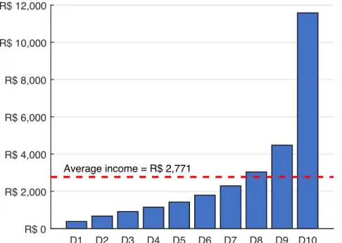
D1 D2 D3 D4 D5 D6 D7 D8 D9 D10 R$ 0 R$ 2,000 R$ 4,000 R$ 6,000 R$ 8,000 R$ 10,000 R$ 12,000 Average income = R$ 2,771
Figure 1: Average household income by decile - Brazil (Source: POF, 2009) Acemoglu et al. (2012) studies how technological progress can be directed in a model with climate restrictions. Golosov et al. (2014) uses a dynamic stochastic general equilibrium model to study optimal taxation of fossil fu-els. For a review of macroeconomic models focusing on climate issues, see Hassler, Krusell, and Smith (2016).
This article consists of four sections besides this introduction. The next section describes the data. Section 3 develops the economic model, and Section 4 discusses how the model is calibrated. Section 5 reports the results from the counterfactual analyses. Finally, Section 6 concludes.
2 Data
Despite decreasing since around 2000, the level of income inequality in Brazil is still very high (Barros, Foguel, and Ulyssea (2007)). Figure 1 reports the average household income (in 2009 reais) for each decile of the Brazilian population, using data from POF. The top decile makes, on average, about 30 times more than the poorest decile.
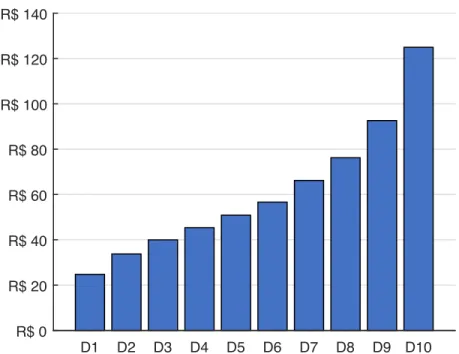
D1 D2 D3 D4 D5 D6 D7 D8 D9 D10 R$ 0 R$ 20 R$ 40 R$ 60 R$ 80 R$ 100 R$ 120 R$ 140
Figure 2: Average monthly energy expenditure by income decile (Source: POF, 2009)
substantial variation in consumption as well. Figure 2 shows energy expen-ditures for each decile. It is easy to see that richer families consume much more energy than their poorer counterparts. Households in the richest decile consume about 5 times more than those in the poorest.
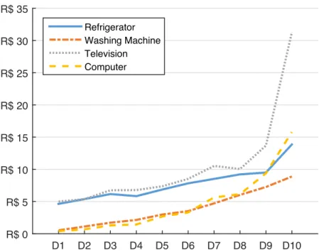
Figure 3 reports the average annual expenditure of each decile on selected electric equipments. Consumption of all of these items increases with income; however, the increases are not proportional. The ratios between the top and bottom deciles are 6:1 for TVs, 3:1 for refrigerators, 17:1 for washing machines, and 40:1 for computers.
D1 D2 D3 D4 D5 D6 D7 D8 D9 D10 R$ 0 R$ 5 R$ 10 R$ 15 R$ 20 R$ 25 R$ 30 R$ 35 Refrigerator Washing Machine Television Computer
Figure 3: Average monthly expenditures on selected electric equipment by income decile (Source: POF, 2009)
By looking at the data described above, one observes great dispersion in both income and expenditures across the different income deciles of the Brazilian population. We also note that energy consumption and expen-ditures on other equipment does not follow increases in income linearly. These observations motivate the theoretical framework that we develop in the next section. To be more precise, the mathematical model will feature non-homothetic utility and heterogeneous agents.
3 Model
This section describes the model with heterogeneous agents. Consider an economy with I agents, heterogeneous with respect to their income yi > 0.
These I income classes can be seen as representing the different income deciles of the Brazilian economy. These families derive utility from the consumption of different goods. There are J + 1 consumption goods; J use energy and 1 does not. Each household values the consumption of these goods according
to the following utility function: log(ci z c) + J X j=1 ↵jlog(sij zj), where si
j is the use of each good j by a family of quantile i. The parameter
↵j represents the weight of each good in the household’s utility, whereas
zc and zj are parameters that control the non-homotheticity of preferences,
imposing a minimal level of consumption for each good. This type of utility function was also used by Bibas et al. (2015) to represent households’ final demand for goods and services, including energy.
The good that does not need energy is the numeraire, with a unitary price. Each of the remaining goods j 2 {1, ..., J} is rented by the household for the price rj. The price of each unit of energy paid by the household
depends on its total energy consumption, Ei, according to p(Ei). The total
service provided by use j is given by sj, and each unit of energy service j
uses tj units of energy. This means that the total energy consumption of the
household i is equal to:
Ei =
J
X
j=1
sijtj.
The household in income quantile i chooses the numeraire ci 2 R + that
it wishes to consume as well as the vector of consumptions of the other J goods, si 2 RJ
+, in order to maximize its utility. The optimization problem
for agent i can thus be described as: max ci,si log(c i z c) + J X j=1 ↵jlog(sij zj) subject to ci+ J X j=1 sij p(Ei)tj+ rj yi Ei = J X sijtj
ci zc, sij zj 8j = 1, . . . , J.
In order to gain some insight about the properties of the model, in the following subsection we discuss the particular case in which the energy tariff is linear. This case is interesting to investigate because there is an analytic solution to it. But in the numerical experiments described in Sections 4 and 5 we will use non-linear tariffs.
3.1 Linear Price of Energy
Let us consider the special case in which the energy price is linear; that is, p(Ei) = p is constant. In order to guarantee the existence of a solution, we
must impose the following restrictions on the parameters: ↵j 0 8j = 1, . . . , J zc+ J X j=1 zj j yi 8i = 1, . . . , I
where j = ptj+rj. The first restriction, on the utility weights ↵j, guarantees
that none of the goods is actually a bad. That is, it guarantees that each good has a positive marginal utility. The second restriction, on the utility costs zc and zj, guarantees that the inequalities ci zc and sij zj are
always true.
Since the model features a Stone-Geary utility function with a linear expenditure system, the optimal quantities can be explicitly obtained from the first order conditions and the budget constraint:
ci = zc+ 1 1 +PJl=1↵l yi zc J X l=1 zl l ! sij = zj+ 1 j ↵j 1 +PJl=1↵l ! yi zc J X l=1 zl l ! 8j = 1, . . . , J. Substituting ci and si in the agent’s objective function, we can write the
Vi = 1 + J X j=1 ↵j ! log yi zc J X l=1 zl l ! J X j=1 ↵jlog ( j) + J X j=1 ↵jlog (↵j) 1 + J X j=1 ↵j ! log 1 + J X l=1 ↵l ! .
Note that, except when zc = 0 and zj = 0 for all j, the indirect utility
is non-separable on income. That is, income non-trivially affects the agent’s decisions. To better illustrate this point, consider the case when J = 1, ↵ = 1, and zc = 0. Figure 4 shows the behavior of the fraction of income spent in
energy. When z1 = 0, the household spends half of its income in energy,
regardless of income level. However, when z1 = 0.1, this fraction depends
on the level of income, approaching 1 when income is low but decreasing back to 0.5 as income level rises. This effect is important, because it allows us to model the heterogeneity of behavior for different levels of income. In particular, price and income elasticities will vary across income levels, being lower in magnitude for lower incomes when zj > 0.
Income (yi) 0 1 2 3 4 5 Share in energy 0 0.2 0.4 0.6 0.8 1 z 1 = 0 z 1 = 0.1
Figure 4: Fraction of income spent in energy
4 Taking the Model to the Data
In order to run the counterfactual analyses, we must first discipline the struc-tural parameters. First, impose J = 12 for the main goods using energy in Brazilian households, namely: the refrigerator, freezer, air conditioner, mi-crowave oven, washing machine, television, electric oven, fan, electric shower, iron, computer and lighting. We assume that each good sj is measured in
units of energy that it uses. We can thus normalize tj = 1 for all j. The
income yi is the average income for each income decile and comes from POF
2008.
We determine the price rj for each good j using the following procedure.
We first obtain the monthly average expenditure for each of the 12 goods for each income decile, using data from POF. We then estimate the monthly energy consumption for each good and each decile, using the simplifying assumption that the period that each good is used and its power are constant across income quantiles. The only variable that changes across deciles is the average ownership. We then compute the percentage of each decile’s
income that is spent on each good, as well as that good’s associated energy consumption.
As for the energy tariff as a function of energy consumption, p(E), Figure 5 describes the average energy tariff for different levels of consumption, using values for Brazil in 2008 (see ANEEL (2017)). The differences between bands of consumption are due to different energy consumption tax rates. Since the tariff bands describe a staircase function, which is not a smooth function because of its discontinuities, our approach was to approximate the function with a cubic polynomial.4
As was mentioned, the electricity demand of the residential sector is com-posed of the sum of the energy requirements of several different pieces of household equipment, which serve different functions. The electricity re-quirement for each of the individual types of equipment was estimated using a Bottom-up model adapted from Januzzi and Swisher (1997). The annual total electricity requirement for each type of household equipment is calcu-lated taking into account the average tenure of the specified equipment, its average power, and its average length of usage per year. The information for the average tenure for equipment within a household for the different income deciles also came from POF 2008. Data from the National Energy Plan (EPE (2008)) and from the Assessment of the Energy Efficiency Market in Brazil—Tenure of Equipments and Their Use Patterns in the Residential Sector (PROCEL (2007)) was used for average power and average usage per year. The data was used to calculate monthly energy consumption and equipment expenditures for different uses and levels of income.
4The resulting polynomial gave us the function p(E) = 1.8205287914064 ⇥ 10 9 ⇥ E3 2.2253130146168⇥ 10 6
⇥ E2+ 0.000922873215071064
Energy consumption (kWh/month) 0 100 200 300 400 500 Energy tariff (R$/kWh) 0.32 0.34 0.36 0.38 0.4 0.42 0.44 0.46 Tariff bands Polynomial approximation
Figure 5: Energy tariff behavior among levels of consumption
We turn now to the structural parameters of the model. Regarding the agents’ preferences, we have 25 parameters, namely:
• (1 parameter) The disutility of non-energy good consumption: zc.
• (12 parameters) The relative preference weight for each energy use: ↵j, j = 1, . . . , 12.
• (12 parameters) The disutility of each energy use: zj, j = 1, . . . , 12.
In order to discipline these parameters, we target 130 statistics in the data: • (120 moments) Monthly equipment expenditures for each of the 12
energy uses and for each income decile.
• (10 moments) Monthly energy consumption for each income decile (10). We take as given the average income for each decile computed using POF 2008 data.
We then adjust the parameters in order to minimize the relative distance between the data moments and their model counterparts. Formally, let ✓ = (↵0, z0)0 be the 25⇥1 vector that contains all preference parameters ↵j, zc, and
zj. Denote by Md the 130 ⇥ 1 vector of data targets used in the calibration,
Mm(✓)the model counterparts given the parameter vector ✓, and W , a weight
matrix. For each descriptive statistic k, the relative deviation between data (Md,k) and model (Mm,k(✓)) statistics is given by
Mm,k(✓) Md,k
Md,k
.
The calibration procedure minimizes the sum of squared relative devia-tions, that is,
ˆ ✓ = arg min ✓ 130 X k=1 ✓ Mm,k(✓) Md,k Md,k ◆2 .
The advantage of using relative deviation instead of absolute deviation is that it compensates for the different magnitudes among the descriptive statistics. For example, the expenditures are much higher for the tenth decile than for the first decile. If we used absolute deviation, we would be giving more weight to deviations in higher income levels than lower levels. Relative deviation compensates for this effect, giving more weight for lower magnitudes.
Equivalently, we can also write down the calibration problem in a matri-cial form: ˆ ✓ = arg min ✓ (Mm(✓) Md) 0W(M m(✓) Md),
where the weighting matrix W is given by:
W = 2 6 6 6 6 6 4 Md,12 0 . . . 0 0 0 Md,22 . . . 0 0 ... ... ... ... ... 0 0 . . . Md,1292 0 0 0 . . . 0 Md,1302 3 7 7 7 7 7 5 .
4.1 Model Fit
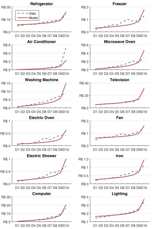
The calibrated parameters are given in Table 1. The comparisons between the data targets and the benchmark model are reported in Figures 6 and 7.
The prefence weight parameters, ↵, are all well below the non-energy goods unitary weight, which is expected since none of these energy uses represents a significant fraction of households’ budgets. Since we assumed that the energy service provided by each use is measured by its energy consumption, we cannot use the weights to compare preferences between uses, because each use has different levels of efficiency.
↵ z Refrigerator 0.00206 21.47993 Freezer 0.00045 2.32375 Air Conditioner 0.00051 0.08928 Microwave Oven 0.00078 0.43872 Washing Machine 0.00154 0.43430 Television 0.00314 6.05674 Electric Oven 0.00016 0.41364 Fan 0.00020 2.46922 Electric Shower 0.00255 12.65511 Electric Iron 0.00035 1.79701 Computer 0.00233 0.24965 Lighting 0.00117 26.98999 Non-energy - 280.87476
Table 1: Parameters of household preferences in the benchmark model On the other hand, we can see that the non-homotheticity parameter, z, is useful for describing differences in expenditures for different income deciles. A higher z means a lower ratio between the consumption of rich and poor deciles. For example, lighting has a high z value (z = 27), but decile 10 only spends 2.4 times more on energy equipment than decile 1. As for air conditioners, z = 0.09, but the equipment expenditure is about 147 times higher for decile 10 than for decile 1. Figures 6 and 7 show that observed and estimated energy consumption and equipment expenditures for each decile are very similar in level, meaning that the model is adequate to describe the heterogeneity of household consumption and can be used as a tool to analyze different policies, which is done in Section 5. Another piece of evidence for the quality of the model is the similarity between the elasticities obtained in the calibrated model and the elasticities described in the literature for Brazil, as discussed in the next subsection.
D1 D2 D3 D4 D5 D6 D7 D8 D9 D10 R$ 0 R$ 20 R$ 40 R$ 60 R$ 80 R$ 100 R$ 120 R$ 140 R$ 160 R$ 180 Data Model
Figure 6: Observed and estimated average monthly energy expenditures by income decile
4.2 Elasticities
As with other papers about the elasticity of the Brazilian household electric energy requirement (Modiano (1984); Schmidt and Lima (2004); Andrade and Lobão (1997); Schutze (2015); Villareal and Moreira (2016)), our results show that the average Brazilian household is relatively inelastic to energy prices and income changes. Therefore, electric energy consumption responds less than proportionally to changes in prices and income. The average elec-tricity price and income elasticity found were, respectively, -0.30 and 0.49, as shown in Table 2.
D1 D2 D3 D4 D5 D6 D7 D8 D9D10 R$ 0 R$ 10 R$ 20 Refrigerator Data Model D1 D2 D3 D4 D5 D6 D7 D8 D9D10 R$ 0 R$ 1 R$ 2 Freezer D1 D2 D3 D4 D5 D6 D7 D8 D9D10 R$ 0 R$ 2 R$ 4 R$ 6 Air Conditioner D1 D2 D3 D4 D5 D6 D7 D8 D9D10 R$ 0 R$ 2 R$ 4 R$ 6 Microwave Oven D1 D2 D3 D4 D5 D6 D7 D8 D9D10 R$ 0 R$ 5 R$ 10 R$ 15 Washing Machine D1 D2 D3 D4 D5 D6 D7 D8 D9D10 R$ 0 R$ 20 R$ 40 Television D1 D2 D3 D4 D5 D6 D7 D8 D9D10 R$ 0 R$ 0.5 R$ 1 Electric Oven D1 D2 D3 D4 D5 D6 D7 D8 D9D10 R$ 0 R$ 1 R$ 2 Fan D1 D2 D3 D4 D5 D6 D7 D8 D9D10 R$ 0 R$ 0.5 R$ 1 Electric Shower D1 D2 D3 D4 D5 D6 D7 D8 D9D10 R$ 0 R$ 0.5 R$ 1 R$ 1.5 Iron D1 D2 D3 D4 D5 D6 D7 D8 D9D10 R$ 0 R$ 10 R$ 20 R$ 30 Computer D1 D2 D3 D4 D5 D6 D7 D8 D9D10 R$ 1 R$ 2 R$ 3 R$ 4 Lighting
Figure 7: Observed and estimated average monthly expenditures on selected electric equipment by income decile
Decile Price Elasticity Income Elasticity D1 -0.01706 0.098083 D2 -0.06525 0.163507 D3 -0.12001 0.246972 D4 -0.14438 0.289849 D5 -0.17775 0.335673 D6 -0.21671 0.389180 D7 -0.26022 0.448933 D8 -0.31148 0.519313 D9 -0.38063 0.614273 D10 -0.51924 0.804621 Average -0.29524 0.494357
Table 2: Price and income elasticities for the calibrated model
However, it is important to note that implied elasticities in the model for energy consumption are quite different across income deciles. Poorer households in Brazil are more inelastic to energy prices and income changes than households from the high-income deciles. Considering electricity price changes, a one percent increase in electricity pricing causes the consumer from the lowest income group (D1) to reduce the energy consumption in their household by just 0.02%, whereas, in the case of households from D10, the reduction of energy consumption is greater than 0.50%.
On the other hand, households tend to be more elastic and respond with more significant energy consumption variations when considering in-come changes than pricing changes. For instance, a one percent increase in income induces an increase of 0.10% in the energy consumption for the low-est income decile (D1), while households in the highlow-est income group (D10) increase their energy consumption by 0.80%.
5 Numerical Results
With the calibrated model, it is possible to perform various counterfactual analyses to infer the impact of different scenarios on the household’s energy demand. We also study the impact of the introduction of more energy-efficient fluorescent light bulbs.
1. A tariff reduction of 40%;5
2. A rise in income of 40%;
Let us first look into the expenditure composition. Figure 8 shows that en-ergy and equipment weigh more heavily on the budgets of poorer deciles, since households in decile 1 (D1) spend 12% of their income on energy and electrical equipment, while for D10 this number is only 2%. If we take a closer look at the different uses that energy is put to, the categories where households spend the most on average are lighting, refrigerators and elec-tric showers. For each income decile, Table 3 illustrates share of each of these three categories as a percentage of total expenditures. It is clear that the share of lighting and refrigerators decreases as income increases, while the inverse is true for electric showers. The expenditure composition for the counterfactual scenarios are displayed in Table 4. It shows that there is little change in the composition over the scenarios, except for decile 1, where equipment and energy expenditures decrease from 12% to 9% in both counterfactuals. D1 D2 D3 D4 D5 D6 D7 D8 D9 D10 0% 5% 10% 15% Energy expenditure Equipment expenditure
Figure 8: Benchmark - energy and equipment expenditures as % of income
5In this scenario, tariff reduction considers the multiplication of the tariff polynomial, p(E), by 0.6.
Decile Lighting Refrigerator Electric Shower D1 27% 31% 11% D2 25% 30% 12% D3 24% 29% 12% D4 23% 27% 13% D5 22% 26% 13% D6 21% 25% 14% D7 19% 24% 15% D8 18% 22% 15% D9 16% 21% 16% D10 12% 17% 18%
Table 3: Use expenditures as % of total equipment and energy expenditures Decile Benchmark Tariff - 40% Income + 40%
D1 12% 9% 9% D2 7% 6% 6% D3 6% 5% 5% D4 5% 4% 4% D5 4% 4% 4% D6 4% 3% 3% D7 3% 3% 3% D8 3% 3% 3% D9 3% 2% 2% D10 2% 2% 2%
Table 4: Equipment and energy expenditures as % of income
As for energy consumption, according to Table 5 and Figure 9, changes are more prominent for higher-income deciles than for lower-income deciles. However, decile 1 responds more substantially to a rise in income (4%, against 1% for the tariff reduction), while decile 10 is more responsive to the tariff change (31%, against 24% in the income change scenario). All deciles increase consumption and, in general, the magnitude of the increase is higher when income is higher, except for decile 4 which has a lower increase than decile 3. The reason for this is the shape of the adjusted tariff polynomial, since the increase would be monotone if the tariff was linear, as shown in Section 3.1.
Decile Tariff - 40% Income + 40% D1 1% 4% D2 4% 5% D3 9% 10% D4 9% 9% D5 11% 10% D6 13% 12% D7 15% 13% D8 19% 16% D9 23% 18% D10 31% 24%
Table 5: Energy consumption (% change from the benchmark)
D1 D2 D3 D4 D5 D6 D7 D8 D9D10 0 kWh 100 kWh 200 kWh 300 kWh 400 kWh 500 kWh Monthly consumption Benchmark Tariff - 40% Income + 40% D1 D2 D3 D4 D5 D6 D7 D8 D9D10 0% 5% 10% 15% 20% 25% 30% Percentage change Tariff - 40% Income + 40%
Figure 9: Energy consumption
We can observe the heterogeneity among the different uses comparing the cases of electric showers, computers and air conditioners (Figure 10). First, the poorest households hardly consume any energy through computers and air conditioners (less than 1 kWh per month), whereas they consume 14 kWh/month via electric showers. In addition, for these poorest families, en-ergy consumption via computers and air conditioners responds more sharply to changes in income than to changes in tariffs. An increase of 40% in the poorest families’ incomes can elevate the energy consumption related to com-puters by 70% and to air conditioners by 90%. On the other hand, the same
income increase would increase the energy consumption related to electric shower by just 7% for the first decile. Although the increase in energy con-sumption of computers and air conditioners is very high for the first decile, it can be explained by the fact that consumption levels are so low for these uses that any small absolute increase leads to a large relative increase.
D1 D2 D3 D4 D5 D6 D7 D8 D9D10 0 kWh 50 kWh 100 kWh 150 kWh Electric Shower Benchmark Tariff - 40% Income + 40% D1 D2 D3 D4 D5 D6 D7 D8 D9D10 0% 20% 40%
60%Electric Shower (percentage change)
Tariff - 40% Income + 40% D1 D2 D3 D4 D5 D6 D7 D8 D9D10 0 kWh 5 kWh 10 kWh 15 kWh 20 kWh 25 kWh Computer D1 D2 D3 D4 D5 D6 D7 D8 D9D10 0% 20% 40% 60%
80%Computer (percentage change)
D1 D2 D3 D4 D5 D6 D7 D8 D9D10 0 kWh 5 kWh 10 kWh 15 kWh Air Conditioner D1 D2 D3 D4 D5 D6 D7 D8 D9D10 20% 40% 60% 80%
100%Air Conditioner (percentage change)
Figure 10: Energy consumption for electric showers, computers and air con-ditioners
The reduction tariff scenario generates more marked results for poorer households. As shown in the Figure 11, the tariff reductions create a re-duction of 40% in the poorest households’ energy expenditures, whereas an
increase of 40% would increase the energy expenditure by nearly 5%.
Therefore, although both scenarios result in more significant changes in the energy consumption of households from the high-income classes, the re-duction in the share of the energy consumption expenditures on overall in-come was more pronounced in the lowest inin-come deciles. As these consumers are more elastic to income changes, the tariff reduction counterfactual results in bigger reductions in the share of energy expenditures compared to total income. Nevertheless, in the case of decile 1, both scenarios generated a reduction in energy consumption expenditures from 11.5% to approximately 8.6% of overall income. In the other deciles, the tariff reduction scenario resulted in even more significant reductions.
D1 D2 D3 D4 D5 D6 D7 D8 D9D10 R$ 0 R$ 50 R$ 100 R$ 150 R$ 200 Monthly expenditure Benchmark Tariff - 40% Income + 40% D1 D2 D3 D4 D5 D6 D7 D8 D9D10 -40% -20% 0% 20% 40% Percentage change Tariff - 40% Income + 40%
Decile Benchmark Tariff - 40% Income + 40% D1 11.5% 8.6% 8.6% D2 7.2% 5.5% 5.9% D3 5.7% 4.6% 4.9% D4 5.0% 4.0% 4.3% D5 4.4% 3.6% 3.8% D6 3.9% 3.2% 3.4% D7 3.4% 2.9% 3.1% D8 3.0% 2.6% 2.8% D9 2.7% 2.4% 2.5% D10 2.2% 2.0% 2.1%
Table 6: Expenditures: Energy and equipment (% of income)
Table 7 analyzes the effective subsidy on energy created by a 40% reduc-tion of the energy tariff. The second column displays the cost, in 2009 US$, for each household of a specific decile. The third column is the change in energy consumption, and the fourth is the fraction between the second and the third column. The fraction shows how much of the subsidy is reverted to non-energy expenditure. These values show that lower deciles allocate most of the subsidy toward non-energy expenditures, while for higher deciles energy consumption is much more sensitive to the price change. As an il-lustration, every 1 US$ of subsidy will increase energy consumption by only 0.13 kWh for decile 1, while for decile 2 this number jumps to 2.54 kWh.
Decile (US$/month)Subsidy Change in energy consumption (kWh/month) Change in energy consumption over subsidy (kWh/US$) Fraction of subsidy reverted to non-energy expenditure D1 6.05 0.76 0.13 96% D2 6.80 3.58 0.53 84% D3 7.70 8.00 1.04 68% D4 8.43 8.18 0.97 71% D5 9.28 10.77 1.16 65% D6 10.46 14.29 1.37 58% D7 12.07 19.02 1.58 51% D8 14.53 26.11 1.80 44% D9 19.32 39.77 2.06 35% D10 42.23 107.13 2.54 23%
Table 7: Subsidy on energy
5.1 Technological Change - Fluorescent Light Bulbs
The model developed here is also capable of analyzing the impact of the adoption of different technologies. For example, here, we consider a scenario where all lighting is provided by fluorescent bulbs, which are a more energy efficient and costly technology than incandescent bulbs. The average level of incandescent and fluorescent bulb possession for the benchmark model was calibrated using Brazilian data from PROCEL (2007). The data shows that Brazilian households had on average 8 light bulbs (4 fluorescent and 4 incan-descent), and that LED lamps were still incipient at that time. Therefore, we only considered full adoption of fluorescent lamp for the counterfactual. Based on the average efficiency level of florescent bulbs when compared to incandescent ones, we assume that full fluorescent lamps usage would, on average, consume only 37% of the energy needed to give the same amount of lighting as the benchmark, thus we set t = 0.37, since we adopted the convention of measuring energy service in kWh/month on the benchmark, setting t to 1. As for the price of fluorescent light bulbs, we used a 92% increase, based on the market price survey conducted for that study.Figure 12 displays the percent changes in energy consumption and ex-penditures, both for lighting and total exex-penditures, across income deciles.
The expenditure for light bulbs increased significantly, by 93% for decile 1 and 159% for decile 10, but the decrease in energy expenditures more than compensated for that. For instance, the combined expenditure on energy and equipment for lighting fell by 42% for decile 1 and 25% for decile 10. Since lighting comprises an important share of households’ energy consump-tion—28% in the benchmark model—the impact of this experiment was not negligible over total expenses. Energy expenditures reduced by 24% for decile 1 and 9% for decile 10, and the combined expenditure in energy and all equip-ment fell by 12% for decile 1 and 3% for decile 10.
D1 D2 D3 D4 D5 D6 D7 D8 D9D10 -100% -50% 0% 50% 100% 150% 200% Lighting Energy consumption Energy expenditure Equipment expenditure
Energy and equipment expenditure
D1 D2 D3 D4 D5 D6 D7 D8 D9D10 -30% -20% -10% 0% 10% 20% Total Energy consumption Energy expenditure Equipment expenditure
Energy and equipment expenditure Figure 12: Fluorescent lighting – percentage changes from benchmark
The non-energy expenditure increased modestly for most deciles, but the impact was relatively more pronounced for poorer households. For decile 1, it increased 1.62%, and for decile 2, 0.87%, as shown in Figure 13. The en-ergy consumption on all uses except lighting increased slightly for all deciles, meaning that all households were better off in this scenario. This result suggests that technological progress that makes equipment more energy ef-ficient, even though it becomes more expensive, may be welfare-enhancing, especially for poorer households.
D1 D2 D3 D4 D5 D6 D7 D8 D9 D10 0% 0.5% 1% 1.5% 2%
Figure 13: Fluorescent lighting – percentage changes on non-energy expen-ditures
6 Concluding Remarks
This paper develops a heterogeneous agent model in which households choose the consumption of different goods that use energy. We calibrated this model using consumption micro data for the Brazilian economy. We also performed different counterfactuals that changed both income and energy prices. One conclusion from our model is that poorer households in Brazil seem to be somewhat inelastic when it comes to energy consumption.
The framework can also be used to study the impact of adopting new technologies. We study how the introduction of more energy-efficient fluores-cent light bulbs affects the demand for energy and the consumption of other goods. The results point to especially important effects among the poorer households in the economy: These households gain from the lower energy expenditures even though the new technology is initially more expensive.
The model developed in this paper can also be used to analyze the impact of different policies, such as the taxation of different goods or energy. More-over, it is also well-suited to studying the adoption of other technologies. We leave these as potential avenues for future research.
References
Acemoglu, D., P. Aghion, L. Bursztyn, and D. Hemous. 2012. “The Envi-ronment and Directed Technical Change.” American Economic Review 102 (1): 131–66.
Achão, C. C. L. 2003. “Análise da Estrutura de Consumo de Energia no Setor Residencial Brasileiro.” mimeo, COPPE/UFRJ/PPE.
. 2009. “Análise de Decomposição das Variações no Con-sumo de Energia Elétrica no Setor Residencial Brasileiro.” mimeo, COPPE/UFRJ/PPE.
Andrade, T. A., and W. J. A. Lobão. 1997. “Elasticidade renda e preço da demanda residencial de energia elétrica no Brasil.” Texto para Discussão IPEA n. 489.
ANEEL. 2017. “Relatórios de Consumo e Receita de Distribuição.”
Arouca, M. C. 1982. “Análise da Demanda de Energia no Setor Residencial no Brasil.” mimeo, COPPE/UFRJ/PPE.
Barros, R. P., M. N. Foguel, and G. Ulyssea. 2007. Desigualdade de renda no Brasil: uma análise da queda recente. Brasília: IPEA.
Bataille, C., M. Jaccard, J. Nyboer, and N. Rivers. 2006. “Towards General Equilibrium in a Technology-Rich Model with Empirically Estimated Behavioral Parameters.” The Energy Journal 27:93–112.
Bibas, R., C. Cassen, R. Crassous, C. Guivarch, M. Hamd-Cherif, J. C. Hourcade, F. Leblanc, A. Mejean, E. O Broin, J. Rozenberg, O. Sassi, A. Vogt-Schilb, and H. D. Waisman. 2015. IMpact Assessment of CLI-Mate policies with IMACLIM-R 1.0. - Model documentation version 1.1.
Bôa Nova, A. C. 1985. Energia e Classes Sociais no Brasil. São Paulo -SP: Ed. Loyola.
Chen, W., Z. Wu, J. He, P. Gao, and S. Xu. 2007. “Carbon emission con-trol strategies for China: A comparative study with partial and general equilibrium versions of the China MARKAL model.” Energy 32 (1): 59–72.
Cohen, C. 2002. “Padrões de Consumo: Desenvolvimento, meio ambiente e energia no Brasil.” mimeo, COPPE/UFRJ/PPE.
Cohen, C., M. Lenzen, and R. Schaeffer. 2005. “Energy requirements of households in Brazil.” Energy Policy 33 (4): 555–562.
DePaula, G., and R. Mendelsohn. 2010. “Development and the impact of climate change on energy demand: Evidence from Brazil.” Climate Change Economics 1 (03): 187–208.
Dias, T. F., et al. 2015. “Elasticidades-preço e renda da demanda domiciliar de eletricidade: estimação econométrica com dados da POF 2008/2009.” Master’s thesis, Programa de Pós-graduação em Economia – Universi-dade Federal de Juiz de Fora.
EPE. 2008. Plano Nacional de Energia 2030. Rio de Janeiro: Ministério das Minas e Energia.
. 2017. Balanço Energético Nacional. Empresa de Pesquisa En-ergética.
Golosov, M., J. Hassler, P. Krusell, and A. Tsyvinski. 2014. “Optimal Taxes on Fossil Fuel in General Equilibrium.” Econometrica 82 (1): 41–88. Hassler, J., P. Krusell, and A.A. Smith. 2016. “Environmental
Macroeco-nomics.” Handbook of Macroeconomics 2:1893 – 2008.
Horne, M., M. Jaccard, and K. Tiedemann. 2005. “Improving behavioral realism in hybrid energy-economy models using discrete choice studies of personal transportation decisions.” Energy Economics 27 (1): 59–77. Jannuzzi, G., and L. Schipper. 1991. “The structure of electricity demand
in the Brazilian household sector.” Energy Policy 19 (9): 879–891. Januzzi, G., and J. Swisher. 1997. Planejamento Integrado de Recursos
Energéticos: meio ambiente,Conservação de energia e fontes renováveis. Campinas: Autores Associados.
Lins, M. P. 1988. “Estrutura do Consumo Energético Residencial no Estado do Rio de Janeiro.” Informação Técnica AESP, vol. 0-001/88.
Mathy, S., M. Fink, and R. Bibas. 2015. “Rethinking the role of scenar-ios: Participatory scripting of low-carbon scenarios for France.” Energy Policy 77:176–190.
Modiano, E. 1984. “Elasticidade-renda e preços da demanda de energia elétrica no Brasil.” Texto para discussão PUC/RJ n. 68.
Infor-Morello, T. F., V. Schmid, and R. Abramovay. 2011. “Rompendo com o trade-off entre combate à pobreza e mitigação do efeito estufa: o caso do consumo domiciliar de energéticos no Brasil.” Technical Report, IPEA, Brasília.
Nordhaus, W., and J. Boyer. 2000. Warming the World: Economic Modeling of Global Warming. Cambridge, MA: MIT Press.
PROCEL. 2007. Avaliação do mercado de eficiência energética no Brasil: Pesquisa de Posse de Equipamentos e Hábitos de Uso - Ano base 2005. Classe Residencial, Relatório Brasil. Rio de Janeiro: Eletrobrás.
Pye, S., and C. Bataille. 2016. “Improving deep decarbonisation modelling capacity for developed and developing country contexts.” Climate Policy 16:27–46.
Rivers, N., and M. Jaccard. 2005. “Combining top-down and bottom-up approaches to energy-economy modeling using discrete choice methods.” The Energy Journal 1:83–106.
Schaeffer, R. 2008. “Elaboração de Ferramenta Computacional para Estimar o Potencial de Conservação de Energia Elétrica em Comunidades de Baixo Poder Aquisitivo.” Relatório Técnico Light.
Schaeffer, R., C. Cohen, M. A. Almeida, C. C. L. Achão, and F. M. Cima. 2003. Energia e Pobreza: Problemas de Desenvolvimento Energético e Grupos Sociais Marginais em Áreas Rurais e Urbanas do Brasil. San-tiago: Unidad de Recursos Naturales e Infraestructura de La Comisión Económica para America Latina y el Caribe (Cepal), Naciones Unidas. Schmidt, C. A. J., and M. A. M. Lima. 2004. “A demanda por energia
elétrica no Brasil.” Revista brasileira de economia 58 (1): 68–98.
Schutze, A. M. 2015. “A Demanda de Energia Elétrica no Brasil.” Ph.D. diss., PUC-Rio.
Shukla, P. R., S. Dhar, and D. Mahapatra. 2008. “Low-carbon society scenarios for India.” Climate Policy 8 (sup1): S156–S176.
Strachan, N., S. Pye, and R. Kannan. 2009. “The iterative contribution and relevance of modelling to UK energy policy.” Energy Policy 37 (3): 850–860.
Vanin, V. R., M. G. Graça, and J. Goldemberg. 1981. “Padrões de consumo de energia - Brasil 1970.” Ciência e Cultura 33 (4): 477–486 (Abril).
Villareal, M. J. C., and J. M. L. Moreira. 2016. “Household consumption of electricity in Brazil between 1985 and 2013.” Energy Policy 96:251–259. Weiss, M. 2015. “Análise do Consumo de Energia Direta e
Indi-reta das Famílias Brasileiras por Faixa de Renda.” Master’s thesis, UFRJ/COPPE.