Review
On Consensus-Based Distributed Blind Calibration
of Sensor Networks
Miloš S. Stankovi´c1,2,3,*, Srdjan S. Stankovi´c2,4, Karl Henrik Johansson5, Marko Beko6,7 and Luis M. Camarinha-Matos7,8
1 Innovation Center, School of Electrical Engineering, University of Belgrade, 11120 Belgrade, Serbia 2 Vlatacom Institute, 11070 Belgrade, Serbia; [email protected]
3 School of Technical Sciences, Singidunum University, 11000 Belgrade, Serbia 4 School of Electrical Engineering, University of Belgrade, 11120 Belgrade, Serbia
5 ACCESS Linnaeus Center, School of Electrical Engineering, KTH Royal Institute of Technology,
SE-100 44 Stockholm, Sweden; [email protected]
6 COPELABS, Universidade Lusófona de Humanidades e Tecnologias, Campo Grande 376,
1749-024 Lisboa, Portugal; [email protected]
7 CTS/UNINOVA, Monte de Caparica, 2829-516 Caparica, Portugal; [email protected]
8 Faculty of Sciences and Technology, NOVA University of Lisbon, 2825-149 Caparica, Portugal
* Correspondence: [email protected]
Received: 25 September 2018; Accepted: 5 November 2018; Published: 19 November 2018
Abstract: This paper deals with recently proposed algorithms for real-time distributed blind macro-calibration of sensor networks based on consensus (synchronization). The algorithms are completely decentralized and do not require a fusion center. The goal is to consolidate all of the existing results on the subject, present them in a unified way, and provide additional important analysis of theoretical and practical issues that one can encounter when designing and applying the methodology. We first present the basic algorithm which estimates local calibration parameters by enforcing asymptotic consensus, in the mean-square sense and with probability one (w.p.1), on calibrated sensor gains and calibrated sensor offsets. For the more realistic case in which additive measurement noise, communication dropouts and additive communication noise are present, two algorithm modifications are discussed: one that uses a simple compensation term, and a more robust one based on an instrumental variable. The modified algorithms also achieve asymptotic agreement for calibrated sensor gains and offsets, in the mean-square sense and w.p.1. The convergence rate can be determined in terms of an upper bound on the mean-square error. The case when the communications between nodes is completely asynchronous, which is of substantial importance for real-world applications, is also presented. Suggestions for design of a priori adjustable weights are given. We also present the results for the case in which the underlying sensor network has a subset of (precalibrated) reference sensors with fixed calibration parameters. Wide applicability and efficacy of these algorithms are illustrated on several simulation examples. Finally, important open questions and future research directions are discussed.
Keywords:blind calibration; macro calibration; distributed estimation; sensor networks; consensus; synchronization; stochastic approximation
1. Introduction
Recently emerged technologies dealing with networked systems, such as the Internet of Things (IoT), Networked Cyber-Physical Systems (CPS), and Sensor Networks (SN), still have many conceptual and practical challenges intriguing to both researchers and practitioners [1–9]. New classes of problems in this area continuously arise, driven by many new real-world applications. Particularly in the
case of SNs, application examples include environment monitoring, wildfires detection, shop-floor manufacturing, smart cities, etc. One of the most important challenges, limiting the performance, robustness and time-to-market of these new technologies, is sensor calibration. Micro-calibration can be performed only in relatively small SNs where every sensor is individually calibrated in a controlled environment. Typical SNs are of large scale, functioning in dynamic and partially unobservable environments, thus demanding new methods and algorithms for efficient calibration. The idea of macro-calibration is to calibrate the entire SN based on the total system response, so that there is no requirement to individually calibrate every sensor node. The typical approach is to formulate the calibration problem as a parameter estimation problem (e.g., [10,11]). Of significant interest are methods for automatic calibration of SNs which successfully perform even if there are no reference signals/sensors, or other sources of groundthruth information about the measured process. In these situations, the goal of the calibration is to achieve homogeneous behavior of all the nodes, possibly enforcing dominant influence of sensors that are a priori known to provide sufficently good (calibrated) measurements. These types of calibration problems are known as the blind calibration problems (e.g., [12]). Furthermore, in many applications of SNs, it is of essential importance that the network functions in a completely decentralized fashion, preforming calibration in real-time, without the requirement for any kind of centralized information fusion. Hence, completely distributed and decentralized real-time calibration algorithms are of paramount importance.
In this paper, we study recently proposed algorithms which possess all the mentioned desirable properties: they deal with blind macro-calibration of SNs based on completely decentralized, real-time and recursive estimation of the parameters of linear calibration functions [13–17]. Another advantageous property of these algorithms is that it is assumed that the underlying SN have directed communication links between neighboring nodes. A basic algorithm is developed by using a distributed optimization problem setup, constructing a distributed gradient recursive scheme, with the local objectives formulated as weighted sums of mean-square differences between the corrected sensor readings of neighboring nodes. A direct consequence of this problem setup is that the algorithm can be studied as a generalized consensus scheme, to which the existing convergence results of standard consensus schemes are not applicable (e.g., [18]). However, by using techniques based on the stability of diagonally quasi-dominant dynamical systems [13,19–21] it is possible to prove asymptotic convergence of calibrated sensor outputs to consensus, in the mean-square sense and with probability one (w.p.1). The basic algorithm can be extended by assuming the presence of several factors which are of essential importance for practical applicability of the proposed method: (1) additive communication noise, (2) communication dropouts, (3) additive measurement noise, and (4) asynchronous communication.
case of only one reference sensor, the corrected gains and offsets of the rest of the sensors converge to the same point imposed by the reference sensor.
Finally, an analysis is given which clarifies the influence of initially selected weights corresponding to particular nodes in the presented calibration parameters estimation recursions. Guidelines are formulated on how these weights should be chosen so that given requirements are satisfied. General discussion of the described results is provided from both theoretical and practical points of view, based on which several future research directions are proposed.
The outline of the rest of the paper is as follows. The following section briefly discusses related work. In Section3we introduce the distributed blind macro-calibration problem and derive the basic algorithm for the noiseless case. Section4is devoted to the presentation of the convergence properties of the base algorithm. In Section5certain assumptions about the measured signals, communication errors, and communication protocol are relaxed, and the appropriate algorithm modifications are introduced, together with their convergence properties. In Section6a discussion on the convergence rate, the case of presence of reference sensors with fixed characteristics, and some design guidelines are presented. In Section7we present illustrative simulation results. Finally, Section8presents some conclusions and future research directions.
2. Related Work
Macro-calibration is based on the idea of calibrating the whole SN based on the responses of all the nodes. The most frequent approaches to this problem are based on parameter estimation techniques (e.g., [11]). If controlled stimuli are not available the problem is usually referred to as blind calibration of SNs. In general, it is a difficult problem, which has certain similarities with more general problems of blind estimation, equalization, and deconvolution (e.g., [22–24] and references therein).
Most of the proposed appraches to blind calibration in the existing literature are centralized and non-recursive [12,25–37]. Within this class of methods, in refs. [12,25] a blind calibration algorithm based on signal subspace projection was analyzed assuming restrictive signal and sensor properties. In ref. [26] the method was improved from the point of view of robustness to subspace uncertainties. In ref. [27] the authors proposed to use sparsity and convex optimization for blind estimation of calibration gains. In ref. [28] an approach to blind sensor calibration is adopted based on centralized consistency maximization at the network level assuming very dense deployment and only pairwise inter-node communications. In ref. [29] a moments-based centralized blind calibration is proposed for mobile SNs, exploiting multiple measurements of the same signal of mobile nodes, assuming that the measured signal does not change in time. In ref. [30], the authors proposed a method which can manage situations in which density requirements are not met. Interesting centralized approaches to blind drift calibration proposed in refs. [31–33], which also work when the density requirement is not met, are based on non-restrictive modeling of the assumed underlying signal subspace, with drift estimation using Kalman filter [31], sparse Bayesian learning [32], or deep learning [33]. The approach in ref. [34] also does not rely on stringent assumptions about signal subspace, but assume first-order auto-regressive signal process model. The authors of [35] introduce linear algebraic model of calibration relationships in a SN with centralized architecture to improve the simple mean calibration scheme, assuming sufficiently dense deployment. Another centralized approach to mobile sensors calibration is proposed in ref. [36] and is based on using a nonnegative matrix factorization. Some of the density assumptions introduced in this work were relaxed in ref. [37]. In ref. [38] the blind calibration problem was treated in a context of sparse sensing, using a message passing algorithm, assuming constant measured signal. The method proposed in ref. [39], based on geospatial estimation and Kalman filter, works if the sensors are calibrated at the beginning of the operation after deployment, and then may start to drift.
neighbors [40–47]. However, these approaches cannot be directly mapped to the calibration problem treated in this paper.
Finally, certain extended consensus algorithms have been applied to SN calibration problems, but in different settings than the one treated in this paper [48–51]. An approach to blind calibration of sensor gains only, based on distributed gossip-based Expectation-Maximization iterations was proposed in ref. [52], assuming that the measured signal is constant. Another distributed approach was proposed in ref. [53], which explicitly uses a state-space model of the underlying process, and a message exchange protocol for offset compensation. The proposed scheme was formulated without proof of convergence. This paper is focused on the algorithms proposed recently in refs. [13–17] representing completely distributed and decentralized blind macro-calibration algorithms with rigorous proofs of convergences for both corrected sensor gains and offsets, with satisfactory performance under diverse deteriorating conditions which may typically appear in practical applications.
3. Problem Definition and the Basic Algorithm
Assume that the SN to be calibrated consists ofnnodes/sensors. In the base setup, it is assumed that each sensor is measuring the same signal x(t) in discrete-time instants t = . . . ,−1, 0, 1, . . .; this signal can be considered as a realization of a stochastic process {x(t)}. Note that we have implicitly assumed that the sensor nodes are functioning synchronously, since all the sensor nodes perform measurements in the same time instancest. We will relax this assumption in Section5.3. The output (measurement) of thei-th node can be written as
yi(t) =αix(t) +βi, (1)
whereαiis the unknown gain, andβithe unknown offset of sensori. Note that, in this problem setup, it is assumed thatαiandβiare unknown constants and not the random variables.
Calibration of a sensor is performed by applying an affine calibration function to the raw readings (1) which results in the following calibrated sensor output
zi(t) =aiyi(t) +bi=gix(t) + fi, (2)
where ai andbi are the calibration parameters to be obtained,gi = aiαi is the corrected gain and fi = aiβi+bithe corrected offset. The calibration objective is, ideally, to find parametersai andbi for whichgiis equal to one and fi equal to zero. In general, if we assume that there are no sensors which give perfect readingszi(t) =x(t)and that the signalx(t)is unknown and cannot be obtained or measured by some other means, this objective is impossible to achieve. Hence, in our decentralized real-time blind macro-calibration problem setup, this ideal objective must be alleviated: we require that the calibration process asymptotically achieves equal calibrated outputszi(t)for all the nodes i=1, ...,n. To approach as close as possible to the ideal goal of achievinggi =1 and fi=0, we could use certain a priori knowledge about the underlying SN, and try to adjust the algorithm, such that, loosely speaking, the “good” sensors (e.g., precalibrated or higher-quality sensors) correct, using the consensus strategy, the response of the rest of the sensors. For example, if, in a given SN, there is an apriori given perfectly calibrated reference sensor, the ideal asymptotic calibration (gi = 1 and
fi=0) of the rest of the sensor nodes will be achieved if the consensus goal is achieved.
Let us now derive the basic calibration algorithm. The idea is to start with local criteria for each node, whose local minimization would lead to a network-level consensus on the corrected sensor outputs:
Ji =
∑
j∈NiγijE{(zj(t)−zi(t))2}, (3)
i=1, ...,n, whereγijare nonnegative scalar weights whose influence on the properties of the algorithm will be discussed later. Denotingθi= [ai bi]T, the following expression is obtained for the gradient of (3):
gradθiJi=
∑
j∈NiγijE
(zj(t)−zi(t))
yi(t)
1
. (4)
From (4) we obtain the following stochastic gradient recursion for estimatingθi∗minimizing (3):
ˆ
θi(t+1) =θˆi(t) +δi(t)
∑
j∈Niγijǫij(t)
yi(t)
1
, (5)
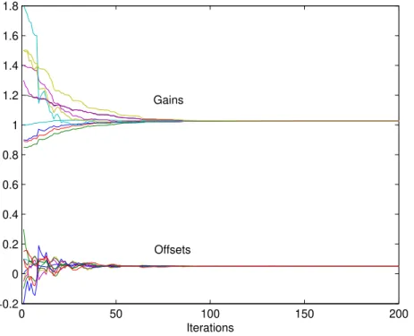
where ˆθi(t) = [aˆi(t) bˆi(t)]T, ǫij(t) = zˆj(t)−zˆi(t), ˆzi(t) = aˆi(t)yi(t) +bˆi(t), and δi(t) > 0 is a time-varying gain whose influence on the convergence properties of the algorithm will be discussed later. The initial conditions are assumed to be ˆθi(0) = [1 0]T,i=1, . . . ,n. We expect that the set of recursions (5) asymptotically achieve that all the local estimates of corrected gains ˆgi(t) =aˆi(t)αiand corrected offsets ˆfi(t) =aˆi(t)βi+bˆi(t)converge to the same values ¯gand ¯f, respectively; this implies that the corrected sensor outputs of all the nodes are also equal ˆzj(t) =zˆi(t),i,j=1, . . . ,n.
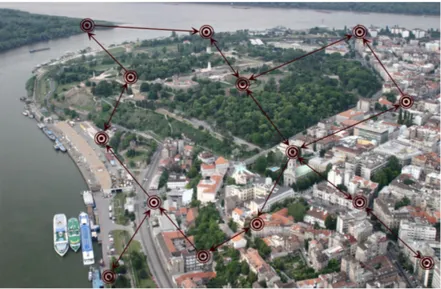
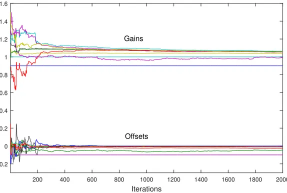
Figure 1.An example sensor network used in smart-city applications with decentralized communication topology. The inter-node communication is performed according to the depicted directed graph. The introduced distributed calibration algorithm achieves asymptotic calibration of all the sensor nodes in the network without using any type of fusion center.
For the sake of compact notations, suitable for convergence analysis of the derived algorithm, let us introduce
ˆ φi(t) =
" ˆ gi(t)
ˆ fi(t)
#
= "
αi 0
βi 1
# ˆ
θi(t), (6)
and
ǫij(t) =
h
x(t) 1i(φˆj(t)−φˆi(t)), (7) so that (5) becomes
ˆ
φi(t+1) =φˆi(t) +δi(t)
∑
j∈NiγijΩi(t)(φˆj(t)−φˆi(t)), (8)
where
Ωi(t) =
"
αiyi(t)x(t) αiyi(t)
[1+βiyi(t)]x(t) 1+βiyi(t)
#
(9)
= "
αiβix(t) +α2ix(t)2 αiβi+α2ix(t)
(1+β2i)x(t) +αiβix(t)2 1+β2i +αiβix(t)
# ,
with the initial conditions ˆρi(0) = [αi βi]T,i=1, . . . ,n. Therefore, the following compact form for the recursions (8) is obtained
ˆ
φ(t+1) = [I+ (∆(t)⊗I2)B(t)]φˆ(t), (10) where ⊗ is the Kronecker product, I is the identity matrix of dimension 2n, I2 is the dimension 2 identity matrix, ˆφ(t) = [φˆ1(t)T· · ·φˆ
n(t)T]T,∆(t) = diag{δ1(t), . . . ,δn(t)}, diag{. . .}denotes the corresponding block diagonal matrix,
B(t) =Ω(t)(Γ⊗I2),
Γ= −
∑
j,j6=1
γ1j γ12 · · · γ1n
γ21 −
∑
j,j6=2
γ2j · · · γ2n
...
γn1 γn2 · · · −
∑
j,j6=n γnj ,
whereγij =0 whenj∈ N/ i, and the initial condition is ˆφ(0) = [φˆ1(0)T· · ·φˆn(0)T]T, according to (8). From the way in which we have constructed the vector ˆφ(t)we conclude that the asymptotic value of
ˆ
φ(t)should be such that all of its odd components are equal, and all of its even components are equal. In the next section, it will be shown that, under certain general assumptions, for any choice of the weightsγij ≥ 0 for j ∈ Ni (and γij = 0 when j ∈ N/ i) the algorithm achieves convergence to consensus. However, if the underlying calibration objective is to achieve absolute calibration of the sensors (i.e., ¯gclose to one and ¯f close to zero), this can be done by trying to exploit sensors that are a priori known to have good characteristics. In a large SN, this can be achieved in two ways: (1) if the large number of sensors are “good” sensors, thenγij-s in all neighborhoodsNishould be approximately the same; or (2) if there is a set of a priori chosen good sensorsj∈ Nf ⊂ N the goal is to enforce their dominant influence to the rest of the nodes. There are two possibilities to achieve this: (a) to set high values ofγijfor allj∈ Nf andi∈ Njout; or (b) to set small values ofγjkfor allj∈ Nf,k∈ Nj,k6=j(which prevents large changes of ˆφj(t)). Section6.3deals with the guidelines on weights tuning, while Section6.4 treats the case in which a set of reference sensors is kept with fixed calibration parameters.
4. Convergence Analysis
In this section we discuss the convergence properties of the calibration scheme presented in the previous section, where it has been assumed that both local sensor measurements and inter-node communications are perfect, i.e., possible communication errors and/or measurement errors are not present. We first analyze this basic scheme in order to focus on structural characteristics of the algorithm; the case of lossy SNs will be treated in the subsequent sections. In the basic setup, without presence of any unreliability, it is sufficient to assume that the step sizesδi(t)are constant:
(A1)δi(t) =δ=const, for alli=1, . . . ,n.
For clearer initial presentation of the convergence results, we now adopt a simplifying assumption: (A2){x(t)}is independent and identically distributed (i.i.d.) sequence, withE{x(t)}=x¯<∞ andE{x(t)2}=s2<∞.
In practice, when the SNs are used to measure certain physical quantities, the assumption that {x(t)}is i.i.d. is almost never satisfied; hence it will be relaxed later.
Based on (A1) and (A2), the expectation of the parameter estimates ¯φ(t) =E{φ(t)}satisfies the following recursion
¯
φ(t+1) = (I+δB¯)φ¯(t), (11) where ¯φ(0) =φ(0), ¯B=Ω¯(Γ⊗I2)and ¯Ω=E{Ω(t)}=diag{Ω¯1. . . ¯Ωn}, with
¯ Ωi =
"
αiβix¯+α2is2 αiβi+α2ix¯
(1+β2i)x¯+αiβis2 1+β2i +αiβix¯
#
. (12)
The following assumption, typical for consensus-based algorithms, is introduced: (A3) GraphGhas a spanning tree.
It implies that the matrixΓhas one zero eigenvalue and the rest eigenvalues with negative real parts, e.g., [54]. Hence, from the structure of matrix ¯B, we directly conclude that it has at least two zero eigenvalues. Its remaining eigenvalues can be characterized starting from the following assumption:
This assumption guarantees that the estimation recursions are sufficiently excited by the signal x(t). Its important consequence is that−Ω¯idefined by (12) is Hurwitz, for alli=1, . . . ,n. Indeed, using some simple algebra it can be derived that−Ω¯iis Hurwitz if and only if (iff)
α2i(s2−x¯2)>0, 2αiβix¯+α2is2+1+β2i >0. (13)
Both inequalities hold iff (A4) holds. This greatly simplifies further derivations which depend on somewhat complicate expression (12) for the 2×2 diagonal blocks of the matrix ¯Ω.
Because of the block structure of matrices ¯Ω and ¯B, the properties of the main recursion (11) cannot be analyzed using standard linear consensus methodologies (see, e.g., [18,54] and references therein). To cope with this problem, a methodology based on the concept of diagonal quasi-dominance of matrices decomposed into blocks has been used [13,17,19–21] to obtain the following important result characterizing all the eigenvalues of the matrix ¯B.
Lemma 1([13,17]). Assume that the assumptions (A3) and (A4) hold. Then, matrixB in (¯ 11) has two zero eigenvalues and the rest eigenvalues have negative real parts.
Observe that vectorsi1= [1 0 1 0 . . . 1 0]T∈R2nandi2= [0 1 0 1 . . . 0 1]T∈R2n, whereR is the set of real numbers, are the right eigenvectors of ¯B corresponding to the eigenvalue at the origin. Letρ1andρ2be the corresponding normalized left eigenvectors, satisfying
ρ 1
ρ2
i1 i2= I2. The following lemma deals with a similarity transformation important for all the remaining derivations throughout the paper.
Lemma 2([13,17]). Let T=hi1 i2 T2n×(2n−2)i, where T2n×(2n−2)is an2n×(2n−2)matrix, such that span{T2n×(2n−2)}= span{B¯}(span{A}denotes a linear space spanned by the columns of matrix A). Then, T is nonsingular and
T−1BT¯ = " 0
2×2 02×(2n−2) 0(2n−2)×2 B¯∗
#
, (14)
whereB¯∗is Hurwitz, and0i×jdenotes a i×j zero matrix.
Notice that
T−1=
ρ1
ρ2 S(2n−2)×2n
, (15)
whereS(2n−2)×2ncan be determined from the definition ofT.
From the structure of the matrices in (11), it can be concluded that the transformationT from Lemma2, when applied to the original matrixB(t), will produce a matrix which has the same structure as the transformed matrix given in Equation (14).
Lemma 3([13,17]). For the matrix B(t)in (10) it holds that, for all t,
T−1B(t)T= " 0
2×2 02×(2n−2) 0(2n−2)×2 B(t)∗
#
, (16)
where B(t)∗is an(2n−2)×(2n−2)matrix and T is given in Lemma2.
Theorem 1([17]). Assume that Assumptions (A1)–(A4) hold. Then there existsδ′>0such that for allδ≤δ′ in (10)
lim
t→∞φˆ(t) = (i1ρ1+i2ρ2)φˆ(0) (17)
in the mean square sense and w.p.1.
Note here that the limit vector in (17)(i1ρ1+i2ρ2)φˆ(0)have all the odd elements equal, and all the even elements equal, which means that the corrected gains of all the nodes converge to the same value, and the corrected offsets of all the nodes converge to the same value. It can be shown [13] that this value only depends on the unknown sensor parametersαiandβi, and the weightsγijinJi, i,j=1, . . .n. For given initial conditions in (5),ρ1φˆ(0)andρ2φˆ(0)are in the form of weighted sums of
αiandβi, 1, . . . ,n, respectively. Assuming that the weightsγijare the same for all the nodes, and that αihave a distribution centered around one, andβiaround zero, these weighted sums will be close to one and zero, respectively.
The value ofδ′ >0 in Theorem1, which ensures convergence, may be restrictive. In practice, the choice of step sizeδin (A1) should be based on the actual properties of the underlying SN; its value needs to be small enough to achieve convergence, but it should also be sufficiently large to achieve acceptable rate of convergence (as in the standard parameter estimation recursions [55]).
After clarifying the main structural properties of the algorithm, we now treat the more realistic case of correlated sequences{x(t)}. We replace (A2) with:
(A2’) The random process{x(t)}is weakly stationary, bounded w.p.1, and with bounded first and second moments, i.e.,|x(t)| ≤ K <∞,E{x(t)}= x¯ <∞,E{x(t−d)x(t)}= m(d) < ∞for all d∈ {0, 1, 2, . . .}(E{·}is a sign of the mathematical expectation),m(0) =s2<∞. It also holds that
(a) |E{x(t)|Ft−τ} −x¯|=o(1), (w.p.1) (18)
(b) |E{x(t−d)x(t)|Ft−τ} −m(d)|=o(1), (w.p.1) (19)
whenτ → ∞, for alld ∈ {0, 1, 2, . . .}, τ > d (Ft−τ denotes the minimalσ-algebra generated by {x(0),x(1), . . . ,x(t−τ)}, ando(1)denotes a function that converges to zero whenτ→∞).
Hence, (A2’) requires stationarity, boundedness, and imposes a mixing condition on the signal {x(t)}. The explicitly used time shift parameterdwill be used later for introducing a new algorithm based on an instrumental variable, capable of dealing with possible measurement noise.
The following theorem examines the convergence of the algorithm (11) under assumption (A2’):
Theorem 2([16]). Assume that the assumptions (A1), (A2’), (A3) and (A4) hold. Then there existsδ′′>0 such that for allδ≤δ′′in (10)limt→∞φˆ(t) = (i1ρ1+i2ρ2)φˆ(0)in the mean square sense and w.p.1.
5. Extensions of the Basic Algorithm
In this section, we introduce several modifications and generalizations of the basic algorithm (5), so that it is possible to achieve distributed calibration under more challenging conditions, typically present in real-life SNs: communication dropouts, additive communication noise, measurement noise, and asynchronous communication. Convergence properties of the introduced modifications are presented in detail.
5.1. Communication Errors
SNs can use analog communication (e.g., when certain types of energy harvesting are used [56]), when additive communication noise is dominant, and dropouts appear less frequently.
The communication errors are formally introduced using the following assumptions:
(A5) The weightsγijin the algorithm (5) are now randomly time-varying, according to stochastic processes given by{γij(t)}={uij(t)γij}, where{uij(t)}are i.i.d. binary random sequences, such that uij(t) =1 with probability pij(pij>0 whenj∈ Ni), anduij(t) =0 with probability 1−pij.
(A6) Instead of receiving ˆzj(t)from the j-th node, thei-th node receives ˆzj(t) +ξij(t), where
{ξij(t)}is an i.i.d. random sequence withE{ξij(t)}=0 andE{ξij(t)2}= (σijξ)2<∞. (A7) Processes{x(t)},{uij(t)}and{ξij(t)}are mutually independent.
Based on the above assumptions, the communication dropout at any iterationt, when nodejis sending to nodei, will happen with probability 1−pij, independently of the additive communication noise process{ξij(t)}and the measured signal{x(t)}.
Denoting
νi(t) =
∑
j∈Ni
γij(t)ξij(t)
"
αiyi(t) 1+βiyi(t)
# ,
andν(t) =hν1(t) . . . νn(t)
i
, one obtains from (10) that
ˆ
φ(t+1) = [I+ (∆(t)⊗I2)B′(t)]φˆ(t) +∆(t)ν(t), (20)
whereB′(t) =Ω(t)(Γ(t)⊗I2), andΓ(t)is obtained fromΓby applying (A5).
Convergence properties of the recursion (20), under the additional assumptions (A5)–(A7), can be derived starting from the results of the previous subsection. Due to the mutual independence of the random variables inB′(t), it can be concluded thatE{B′(t)}=B¯′=Ω¯(Γ¯⊗I2), where ¯Γ=E{Γ(t)}is the same asΓbut withγijreplaced byγijpij. Also, it follows that ˜B′(t)=. B′(t)−B¯′, is a martingale difference sequence (sinceE{B˜′(t)|Ft−1}=0). Furthermore, it can be concluded that ¯B′=Ω¯(Γ¯⊗I2) has the same spectrum as ¯Bin (11): it has two zero eigenvalues and the rest eigenvalues are with negative real part.
Since the additive noise is now present in the recursions (20), (A1) needs to be replaced with the following assumption, typical in the stochastic approximation literature (e.g., [57]):
(A1’)δi(t) =δ(t)>0,∑∞t=0δ(t) =∞,∑∞t=0δ(t)2<∞,i=1, . . . ,n.
Intuitively, (A1’) introduces diminishing gainsδi(t)which converge to zero slowly enough, so that the additive noise can be averaged out while asymptotic convergence to a consensus point is achieved (despite the presence of noise).
Therefore, we have
ˆ
φ(t+1) = (I+δ(t)B¯′)φˆ(t) +δ(t)B˜′(t)φˆ(t) +δ(t)ν(t). (21)
Similarly as in the noiseless case, let as introduce the similarity transformation
T′=hi1 i2 T2′n×(2n−2) i
,
whereT2′n×(2n−2)is an 2n×(2n−2)matrix, such that span{T2′n×(2n−2)}=span{B¯′}. Then,(T′)−1=
ρ′1 ρ′2 S′(2n−2)×2n
, whereρ
′
1andρ′2are the left eigenvectors of ¯B′corresponding to the eigenvalue at the
Theorem 3([13,17]). Let Assumptions (A1’), (A2)–(A7) be satisfied. Then,φˆ(t)generated by (21) converges to i1w1+i2w2in the mean square sense and w.p.1, where w1and w2are scalar random variables satisfying E{w1}=ρ′1φˆ(0)and E{w2}=ρ′2φˆ(0).
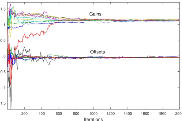
The theorem essentially states that, again, all the corrected drifts converge to the same point, and all the corrected offsets converge to the same point; however, because of the additive communication noise, these points are random and depend on the noise realization. The mean values of these possible convergence points depend on the sensor parametersαiandβi, the design parametersγij, as well as on the dropout probabilitiespij,i,j=1, . . .n.
5.2. Measurement Noise
In this subsection we, in addition to communication errors, assume that the signalx(t)is measured with additive measurement noise. This situation is of essential importance for practical applications since practically all the existing sensors contain certain measurement errors which are typically modeled using stochastic processes [3].
Formally, we model the additive noise stochastic process using the following assumption: (A8) Instead ofyi(t)given by (1), the sensor measurements are now contaminated by noise, and given by
yηi(t) =αix(t) +βi+ηi(t),
where{ηi(t)},i=1, . . .n, are zero mean i.i.d. random sequences withE{ηi(t)2}= (σiη)2, independent of the measured signalx(t).
By replacingyηi(t)instead ofyi(t)in the base algorithm (5), one obtains the following “noisy” version of (8):
ˆ
φi(t+1) =φˆi(t) +δi(t)
∑
j∈Niγij{[Ωi(t) +Ψi(t)][φˆj(t)−φˆi(t)] +Nij(t)φˆj(t)−Nii(t)φˆi(t)}, (22)
where Ψi(t) = ηi(t)
"
αix(t) αi βix(t) βi
#
, Nij(t) =
ηj(t)
αj "
αiyi(t) 0 βiyi(t) 0
# +
ηj(t)ηi(t)
αj 0
0 0
and Nii(t) =
ηi(t)
αi "
αiyi(t) 0 βiyi(t) 0
# +
ηi(t)2
αi 0
0 0
, assumingαi 6= 0, i = 1, ...,n. It is important to observe here that
E{Ψi(t)}=0,E{Nij(t)}=0; howeverE{Nii(t)}=
(σiη)2
αi 0
0 0
.
Assuming again that the step sizesδi(t),i=1, . . . ,n, satisfy (A1’), one can obtain the following equation analog to (10):
ˆ
φ(t+1) = (I+δ(t){[Ω(t) +Ψ(t)](Γ⊗I2) +N˜(t)})φˆ(t), (23)
whereΨ(t) =diag{Ψ1(t), . . . ,Ψn(t)}and ˜N(t) = [N˜ij(t)]with ˜Nij(t) =−∑k,k6=i γikNii(t)fori = j and ˜Nij(t) =γijNij(t)fori6=j,i,j=1, . . . ,n.
In an analogous way as in the previous section, instead of (11), the following equation is obtained for the mean of the corrected calibration parameters
¯
where ¯Bis as in (11) andΣη =−diag{(σ1η)2
α1 ∑jγ1j, 0, . . . ,(σ
η
n)2
αn ∑jγnj, 0}. Because of the additional term Ση, the sums of the rows of the matrix ¯B+Σηare not equal to zero anymore, so that the convergence to consensus (as in Theorem1) cannot be achieved in this case.
However, it can be seen from the structure of the recursion (24) that, if we assume that the measurement noise variances (σiη)2 are a priori known, we can use them to modify the basic algorithm (5) in the following way, ensuring again the asymptotic convergence to consensus:
ˆ
θi(t+1) =θˆi(t) +δ(t){
∑
j∈Niγijǫηij(t)
" yηi(t)
1 #
+
(σiη)2
∑
j∈Ni
γij 0
0 0
θˆi(t)}, (25)
whereǫijη(t) =zˆηj(t)−zˆηi(t)and ˆzηi(t) =aˆi(t)yηi(t) +bˆi(t),i=1, . . . ,n.
The following theorem deals with the convergence of the above modification of the basic algorithm, when the measurement noise is present together with the communication errors. The convergence points will again depend on the measurement and communication noise realizations, in a similar way as in Theorem3.
Theorem 4([17]). Assume that the assumptions (A1’), (A2)–(A8) hold. Then,φˆ(t), given by (25), converges to i1w1+i2w2in the mean square sense and w.p.1, where w1and w2are scalar random variables satisfying E{w1}=ρ′1φˆ(0)and E{w2}=ρ′2φˆ(0).
Notice that the above theorem was based on assumption (A2): indeed, when both{x(t)}and {ηi(t)}are i.i.d. sequences, it is not surprising that the asymptotic consensus is achievable only providedσiη,i=1, . . . ,n, are known. However, we can replace the unrealistic assumption (A2) with (A2’) (introduced in Section4in the noiseless case) allowing correlated sequences{x(t)}which is almost always the case in practice. In such a way, the correlatedness problem present in the algorithm (24) can be overcame, without requiring any a priori information about the measurement noise process. The idea is to introduce instrumental variables in the basic algorithm in the way analogous to the one often used in the field system identification, e.g., [60,61]. Instrumental variables have the basic property of being correlated with the measured signal, and uncorrelated with noise. If{ζi(t)}is the instrumental variable sequence of thei-th agent, one has to ensure thatζi(t)is correlated withx(t)and uncorrelated withηj(t),j=1, . . . ,n. Under A2’) a logical choice is to take the delayed sample of the measured signal as an instrumental variable, i.e., to takeζi(t) =yηi(t−d), whered≥1. Consequently, we present the following general calibration algorithm based on instrumental variables able to cope with measurement noise:
ˆ
θi(t+1) =θˆi(t) +δ(t)
∑
j∈Niγijǫηij(t)
"
yηi(t−d) 1
#
, (26)
where d ≥ 1 and ǫijη(t) = zˆjη(t)−zˆηi(t), ˆzηi(t) = aˆi(t)yηi(t) +bˆi(t), i = 1, . . . ,n. Following the derivations from Section3, one obtains from (26) the following relations involving explicitlyx(t)and the noise terms:
ˆ
φi(t+1) =φˆi(t) +δ(t)
∑
j∈Niγij{(Ωi(t,d) +Ψi(t,d))(φˆj(t)−φˆi(t))
+Nij(t,d)φˆj(t)−Nii(t,d)φˆi(t)}, (27)
where
Ωi(t,d) =
"
αiβix(t) +α2ix(t)x(t−d) αiβi+α2ix(t−d)
(1+β2i)x(t) +αiβix(t)x(t−d) 1+β2i +αiβix(t−d)
Ψi(t,d) =ηi(t−d)
"
αix(t) αi βix(t) βi
# ,
Nij(t,d) = ηj(t)
αj
"
αiyi(t−d) 0 βiyi(t−d) 0
#
+
ηj(t)ηi(t−d) αj 0 0 0 and
Nii(t,d) = ηi( t)
αi
"
αiyi(t−d) 0 βiyi(t−d) 0
#
+
ηi(t)ηi(t−d) αi
0
0 0
.
In the same way as in (23), we have
ˆ
φ(t+1) = (I+δ(t){[Ω(t,d) +Ψ(t,d)](Γ⊗I2) +N˜(t,d)})φˆ(t), (28)
where Ω(t,d) = diag{Ω1(t,d), . . . ,Ωn(t,d)}, Ψ(t,d) = diag{Ψ1(t,d), . . . ,Ψn(t,d)}, ˜N(t,d) = [N˜ij(t,d)], where ˜Nij(t,d) = −∑k,k6=i γikNii(t,d) for i = j and ˜Nij(t,d) = γijNij(t,d) for i 6= j, i,j=1, . . . ,n.
To formulate a convergence theorem for (28), the following modification of (A4) is needed: (A4’)m(d)>x¯2for somed=d0≥1.
This assumption implies that the correlationm(d0)should be large enough. Similarly as in the case of (A4), it can be concluded that (A4’) implies that−Ω¯(d) =−E{Ωi(t,d)}is Hurwitz. Similarly as in the above cases, let as introduce the similarity transformation
T′′=hi1 i2 T2′′n×(2n−2)i,
where T2′′n×(2n−2) is an 2n×(2n−2) matrix, such that span{T2′′n×(2n−2)} = span{B¯(d)′′}. Then,
(T′′)−1 =
ρ′′1 ρ′′2 S(2′′n−2)×2n
, where ρ′′1 and ρ′′2 are the left eigenvectors of ¯B(d)′′ = E{Ω(t,d)(Γ(t)⊗
I2)} = Ω¯(d)(Γ¯ ⊗I2)corresponding to the zero eigenvalue. The following theorem deals with the convergence of the instrumental variable algorithm (26). The convergence point, again, depends on the noise realization.
Theorem 5([16]). Assume that the assumptions (A1’), (A2’), (A3), (A4’), (A5)–(A8) hold. Thenφˆ(t), given by (28) with d=d0, converges to i1w1+i2w2in the mean square sense and w.p.1, where w1and w2are scalar random variables satisfying E{w1}=ρ′′1φˆ(0)and E{w2}=ρ2′′φˆ(0).
5.3. Asynchronous Broadcast Gossip Communication
in which there is less traffic in the city. These types of situations are rigorously treated in the rest of this subsection.
Instead of the problem setup introduced in Section3, assume now that the sensors are measuring a continuous-time signalx(t)at discrete pointstk,tk ∈ R+,k = 1, 2, . . .,tk+1 > tk, producing the sensor outputs
yi(tk) =αix(tk) +βi+ηi(tk), (29) where theαiandβiare the same unknown parameters as in the previous subsections, and we also assume that the measurement noiseηi(tk),i=1, . . . ,n, is present in the sensor readings.
Furthermore, since the goal is to remove dependence on a common global clock, it is now assumed that every nodej∈ Nhas its own local clock. For the sake of compact notation and simpler derivations, a single clock, called global virtual clock, is introduced, which ticks when any of the local clocks ticks. Hence,tkin (29) can be considered as the time in which thek-th tick of the virtual clock happend. To have a well defined situation, it is formally assumed that the ticks of the local clocks are independent, and that the intervals between any two consecutive ticks are finite w.p.1. It is also assumed, for the sake of simpler derivations, that the unconditional probability that thej-th clock ticked at an instance tkisqj>0, independently ofk. It is easy to verify that these conditions are satisfied for a typical model used in SNs, where it is assumed that the local clocks tick according to independent Poisson processes with ratesµj (as in, e.g., [62,63]). This case will be adopted throughout this subsection. It directly follows that, in this case, the virtual global clock ticks according to a Poisson process with the rate ∑nj=1µj.
According to the above assumptions, let us denote withtjlthe ticks of the local clockj,l=1, 2, . . .. The communication protocol can then be defined in the following way. At each local clock tick, a node
jmakes the local sensor measurement, calculates the corrected sensor outputzj(tlj)(based on the current estimates of calibration parametersajandbj), and broadcasts it to its out-neighborsi∈ Njout. We assume also that communication dropouts can happen, i.e., each nodei ∈ Njout receives the transmitted message with probabilitypij >0. For the sake of clarity of presentation, we do not treat additive communication noise in this subsection. It is also assumed that the communication delay is negligible, so that, practically at the same time instant all the nodes which have received the broadcast, perform the local sensor reading, calculate their corrected outputszi(tjl), and update the local estimates of their calibration parametersaiandbi. This procedure is repeated for any local clock tick. The index of the node whose clock has ticked at instanttkis denoted by j(k), and letJ(k)be the subset of the out-neighborsi∈ Njout(k)which have received the broadcast message. Also, letx(k) =x(tk) =x(tlj(k)), yi(k) = yi(tk) = yi(tlj(k)),yj(k) = yj(tk) = yj(k)(tjl(k)),zi(k) = zi(tk) = zi(t
j(k)
l ),zj(k) = zj(tk) = zj(k)(t
j(k)
l ),ηi(k) =ηi(tk) =ηi(t j(k)
l )andηj(k) =ηj(tk) =ηj(k)(t j(k)
l )for somel.
The measurement noise is treated as in the previous subsection, by using the delayed measurement yi(di(k))as the instrumental variable
ζi(k) =yi(di(k)), (30)
wheredi(k)is the global iteration number that corresponds to the closest past measurement of the nodei. By using the same local criteria as in (3) and gradients as in (4), the following new recursion for updating the calibration parameters at nodeiis formulated:
ˆ
θi(k) =θˆi(k−1) +δi(k)γi,j(k)ǫi,j(k)(k)
yi(di(k)) 1
, (31)
where:
• δi(k)is the step size given by δi(k) = νi(k)−c, whereνi(k) = ∑km=1I{i ∈ J(m)}is the number of parameter updates of node i up to the iteration k, with 1/2 < c ≤ 1 (I{·} denotes the indicator function),
• ǫi,j(k)(k) =zˆj(k)(k)−zˆi(k), where
ˆ
zj(k)(k) =aˆj(k)(k−1)yj(k)(k) +bˆj(k)(k−1), (32) ˆ
zi(k) =aˆi(k−1)yi(k) +bˆi(k−1) (33)
are the corrected outputs of nodej(k)and nodei.
The initial conditions are adopted to be ˆθi(0) = [1 0]T. Note that, according to the problem setup, at a given iterationkonly the nodesi∈ J(k)perform the above parameters update; for the rest of the nodes it holds that ˆθi(k) =θˆi(k−1).
Computationally, the algorithm is as simple as the basic one, requiring only a few additions and multiplications in one iteration. Information needed at nodeiare: the local sensor measurement, the local instrumental variable, and the current output sent by an in-neighborj. Knowledge of the global iteration indexk(ordi(k)) is not needed.
From the above definition of the step sizeδi(k)it can be concluded that it depends only on the number of local clock ticks, which makes the algorithm completely decentralized.
It should also be noticed that the instrumental variables in (31) can be selected in several ways. For example, instead of choosing (30), it can be practical to chooseζi(k) =yi(t¯lj,i), where ¯t
j,i
l is the time instant of a supplementary measurement of nodei, just after the last step of the recursion (31) has been locally performed. This scheme is not assumed in the sequel, because of much more complicated notation; all the results can be easily transferred to this case.
Similarly as in the synchronous case, we introduce:
ˆ φi(k) =
" ˆ gi(k)
ˆ fi(k)
#
= "
αi 0
βi 1
# ˆ
θi(k), (34)
and
ǫi,j(k)(k) = h
x(k) 1i(φˆj(k)(k)−φˆi(k)) +aˆj(k)(k)ηj(k)(k)−aˆi(k)ηi(k). (35)
Consequently, we have
ˆ
φi(k) =φˆi(k−1) +δi(k)γi,j(k){(Ωi(k) +Ψi(k))(φˆj(k)(k−1)−φˆi(k−1))
+Ni,j(k)(k)φˆj(k)(k−1)−Nii(k)φˆi(k−1)}, (36)
where
Ωi(k) =
"
αiβix(k) +α2ix(k)x(di(k)) αiβi+α2ix(di(k))
(1+β2i)x(k) +αiβix(k)x(di(k)) 1+β2i +αiβix(di(k))
#
Ψi(k) =ηi(di(k))
"
αix(k) αi βix(k) βi
# ,
Ni,j(k)(k) =
ηj(k)(k)
αj(k) "
αiy0i(di(k)) 0 βiy0i(di(k)) 0
# +
ηj(k)(k)ηi(di(k)) αj(k)
0 0 0 and
Nii(k) = ηi(k) αi
"
αiy0i(di(k)) 0 βiy0i(di(k)) 0
# +
ηi(k)ηi(di(k)) αi
0
0 0
wherey0i(k) =αix(k) +βi, with the initial conditions ˆφi(0) = [αi βi]T,i∈ J(k). Recursions (36) fori=1, ...,n, can be written compactly as
ˆ
φ(k) ={I+ [Ω(k) +Ψ(k)](∆(k)Γ(k)⊗I2) + (∆(k)⊗I2)N˜(k)}φˆ(k−1), (37)
where:
• φˆ(k) = [φˆ1(k)T. . . ˆφn(k)T]T,
• ∆(k) =diag{δ1(k), . . . ,δn(k)},
• Ω(k) =diag{Ω1(k), . . . ,Ωn(k)},
• Γ(k) = [Γ(k)lm], withΓ(k)ll =−γl,j(k)andΓ(k)l,j(k)=γl,j(k)for alll∈ J(k),Γ(k)lm=0, otherwise,
• Ψ(k) =diag{Ψ1(k), . . . ,Ψn(k)},
• N˜(k) = [N˜lm(k)], where ˜Nll(k) = −γl,j(k)Nll(k)and ˜Nl,j(k)(k) =γl,j(k)Nl,j(k)(k), for alll ∈ J(k), ˜
N(k)lm=0, otherwise.
The initial condition is ˆφ(0) = [φˆ1(0)T. . . ˆφn(0)T]T= [[α1β1]T. . .[αn βn]T]T.
Since we have formulated a slightly different problem setup than in Section3, we introduce a new set of assumptions, and denote them using letter B:
(B1){x(k)}is a stationary random sequence, bounded w.p.1, and satisfying theφ-mixing condition. (B2) Let {ti,l}, l = 1, 2, ... represent time instants in which node i performs measurements. Then, minir¯i>m2, wherem=E{x(k)}and ¯ri =E{x(ti,l)x(ti,l−1)},i=1, . . . ,n.
(B3) GraphGhas a spanning tree.
(B4){ηi(k)},i =1, . . .n, are zero-mean sequences of independent and bounded w.p.1 random variables. {ηi(k)}is independent of the process{x(t)}, withE{ηi(k)2}= (σiη)2for allk.
Assumptions (B3) and (B4) are essentially the same as (A3) and (A8).
Theφ-mixing condition (B1) represents one of the strong mixing conditions, usually satisfied for sensory signals [64–66].
Assumption (B2) represents an extension of the assumption (A4), adapted to the presence of the instrumental variableyi(di(k))in (31). It guarantees the persistence of excitation in the sense that the variance ofx(k)must be greater than zero (for allk, because of stationarity) so that constant signals are not allowed [13,55]. However, it also ensures sufficent correlation between the instrumental variable and the current measurement, so that e.g., white noise signals are also not allowed. It can be easily derived [14] that (B2) is satisfied if the autocovariance function ofx(t)is positive in a sufficiently large interval around zero. Also, if the ratesµjare adjustable we can chooseµmin=minj∈Nµjlarge enough, such that (B2) is always satisfied. Therefore, (B2) is, in general, not restrictive for processes having dominant low frequency spectrum, which is typical in practical applications of SNs.
Based on the above modified problem definition, the following result was proved in ref. [14], stating that both corrected gains and corrected offsets will converge to consensus points (which depend on the realizations of the stochastic processes) for all the nodes.
Theorem 6([14]). Let Assumptions (B1)–(B4) be satisfied. Thenφˆ(k)given by (37) converges toφˆ∞=χ1i1+
χ2i2in the mean square sense and w.p.1, whereχ1andχ2are random variables with bounded second moments.
6. Discussion
6.1. Rate of Convergence
Theorem 7([17]). Under the assumptions of any of the Theorems3, 4or5, together withlimt→∞(δ(t+
1)−1−δ(t)−1) =d ≥0, there exists such a positive numberσ′ <1that for all0<σ<σ′the asymptotic consensus is achieved by the presented algorithms with the convergence rate o(δ(t)σ).
It might be problematic to obtain the precise value ofσ′in concrete applications. However, it can be shown that it directly depends on the sensor and network properties (encoded by matrixB(t) orB(t,d)) and on the connectivity of the underlying communication graph [67]. On one hand, if the number of nodes is increased without increasing network connectivity, the rate of convergence will decrease; however, if the graph connectivity is increased, the convergence rate will also increase. For example, if the graph is fully connected, the convergence rate will be high at the expense of very large number of communication links. In practice, a compromise between the rate of convergence and the network complexity needs to be found.
Another compromise to be found is between algorithm’s noise immunity and convergence rate. Indeed, according to [68], assuming thatδ(t)is given asδ(t) =m1/(m2+tµ),m1,m2>0, 1
2<µ≤1, the values ofµcloser to12 give larger rate of convergence but higher sensitivity to noise; the values of µcloser to 1 give the opposite effect.
6.2. Stationarity of the Measured Signal
In the previous section, we made comments about all the introduced assumptions, explaining their practical applicability. Let us make some additional comments on the stationarity assumption for the random process{x(t)}, introduced in (A2), (A2’) and (B1). From the point of view of applications, it cannot be considered restrictive, since it encompasses a large variety of quickly and slowly varying real signals. This assumption is not essential for proving convergence of the presented algorithms: it has been introduced primarily for the sake of focusing on the essential structural aspects of the algorithm and avoiding complex notation [13,14,17]. Notice, according to Lemmas2and3, that the similarity transformationTcan be applied even in the case of time varying matrix ¯B(t), owing to its
specific structure; namely, we haveT−1B¯(t)T= " 0
2×2 02×(2n−2) 0(2n−2)×2 B¯(t)∗
#
, where ¯B(t)∗is Hurwitz and
Tis obtained from ¯B(t)for any selectedt=t′. Moreover, notice that the conclusions of Theorem1 hold, in general, provided the following unrestrictive condition holds: limt∏τ(I−B¯(t−τ)∗) =0.
Also, it is possible to conclude directly that the results of the above theorems hold for changes of ¯B(t)∗ sufficiently slow. Moreover, it is not difficult to prove that the above convergence results exactly hold when the signal is asymptotically stationary.
6.3. Network Weights Design
As already discussed in the previous subsections, the implicit goal of the presented calibration scheme is to exploit the sensors with a priori good calibration properties by enforcing their dominating effect in the final consensus value to which all the nodes converge. This can be done in two ways, by adjusting the design weightsγij: (1) if the majority of sensors are “good”, we can set allγijfor the neighborhood of any nodeito the same value; or (2) if there is a smaller subsetNf ⊂ N of a priori “good” sensors in the network we should appropriately tune the values ofγij. For this scenario, in this subsection, we give a more detailed analysis of the weights adjusting problem for the case of asynchronous communications treated in Section5.3.
According to the theoretical results presented in detail in ref. [14], the dominant component of the random variables[χ1χ2]in Theorem6is given by a weighted sum of the unknown sensor parameters
1. By reducing the values of all the elements in thei-th row of ¯Γ, or
2. By increasing the values γji, j 6= i, from the i-th column (keeping in mind that ¯Γ must be row stochastic).
Probabilitiesqjcan in certain situations also be adjusted since they depend on the rate of the local clock of nodej. By increasing the clock rate of the nodej, the influence of that node on the asymptotic calibration parameter values achieved at consensus, is also increased. Adjusting dropout probabilities 1−pjimight also be possible in certain situations: by decreasing the probability of a nodeiof receiving a message from a neighbor, we increase its influence on the asymptotic consensus. Hence, there are several design variables which can be adjusted so that the desired convergence point is achieved.
6.4. Macro Calibration for Networks with Reference Nodes
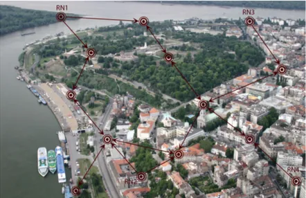
As discussed in the previous subsection, the selection of the weights in the matrix ¯Γis important for attaining the calibration goal of emphasizing a priori selected “good” sensors (“leaders”). Besides the described methods, this can be ultimately done by leaving the nodes from a setNf ⊂ N with unchanged calibration parameters (reference nodes), and only apply the recursions (31) (or (5), or (26)) to the rest of the nodesi∈ N − Nf. An example of a SN with such topology corresponding to the smart city example in Figure1is shown in Figure2.
Figure 2.An example sensor network used in smart-city applications with multiple (four) reference nodes. The reference nodes (RNs) have fixed calibration parameters: only the rest of the nodes implement the given distributed sensor calibration recursions.
In practice, this situation emerges, for example, when a SN needs to be expanded, i.e., when several uncalibrated sensors needs to be added to an already calibrated SN. In this subsection, the convergence results for this case are presented assuming asynchronous calibration algorithm [14].
First, we treat the special case in which|Nf|=1, i.e., there is only one reference sensor, and we want to calibrate the rest of the SN so that their calibrated outputs converge to the output of the reference sensor. For this case, all of the above results still hold, since the resulting communication graph will again have a spanning tree (with the reference node as a center node), which implies that (B3) (and (A3)) holds. Therefore, by applying the above convergence theorems, one concludes that the corrected gains and offsets ˆφi(k),i=1, . . . ,n, will converge to the same value, dictated by the “leader”.
In the general case, assume, without loss of generality, thatNf ={1, 2, . . . ,n
f},nf =|Nf|>0, is the set of reference senors which have fixed parameters: φif =
gif fif
, i ∈ Nf. Assume that ¯