Application of Empirical Mode Decomposition (EMD) to
chronological series of active fires from MODIS satellite
Ana Raquel Dias Tomás
Dissertação para obtenção do Grau de Mestre em
Engenharia Florestal e dos Recursos Naturais
Orientador: Doutor José Miguel Oliveira Cardoso Pereira
Co-Orientador: Licenciado Bernardo Wildung Cantante Mota
Júri:
Presidente: Doutor Manuel Lameiras de Figueiredo Campagnolo, Professor Associado do Instituto Superior de Agronomia da Universidade Técnica de Lisboa
Vogais: Doutor José Miguel Oliveira Cardoso Pereira, Professor Catedrático do Instituto Superior de Agronomia da Universidade Técnica de Lisboa
Doutor Carlos Portugal da Câmara, Professor Associado da Faculdade de Ciências da Universidade de Lisboa
i
ABSTRACT
Fire is a global phenomenon, acting as an important disturbance process. Africa is one of the continents that has higher fire density, particularly in savanna regions, making it the subject of innumerous studies about fire regime and behavior. Here, a new method of time series analysis called Empirical Mode Decomposition (EMD) was applied to monthly fire counts time series from MODIS Terra/Aqua sensors. The goals were to analyze the differences between the time series from the two instruments (MODIS Terra and Aqua), the differences in the behavior of the active fire time series from the north and south parts of Africa and they‟re relationships with climatic modes (ENSO and IOD). For most of the time series, the application of the EMD resulted in four IMF‟s and a residue. Although there is always an IMF related with seasonality, the physical meaning of the other isn‟t clear. This may be due to various reasons, some related with intrinsic problems of the method, other with the applicability of the method to this type of series.
ii
RESUMO
O fogo é um fenómeno global, actuando como um importante processo de perturbação. África é dos continentes que tem maior densidade de fogos a nível global, particularmente nas regiões de savana, tornando-o objecto de inúmeros estudos sobre regimes e comportamentos de fogo. Aplicou-se um novo método de análise de séries temporais, Decomposição de Modo Empírico (EMD), a séries mensais de contagens de fogos activos do sensor MODIS Terra/Aqua. O objectivo passou pela análise das diferenças entre as séries temporais dos dois instrumentos, Terra e Aqua, das diferenças entre o comportamento das séries de fogos activos no norte e sul de África, as relações com modos climáticos, particularmento o ENSO e o IOD, a existência de uma tendência. A aplicação do EMD resultou em quatro IMFs e um resíduo para a maioria das séries. Apesar de haver sempre uma IMF relacionada com a sazonalidade, o significado físico das restantes não é claro. Isto pode ser devido a diversas razões, algumas relacionadas com problemas intrínsecos do método, outras com a própria aplicabilidade do método a este tipo de séries.
iii
RESUMO ALARGADO
O fogo é um fenómeno global, actuando como um importante processo de perturbação. Recentemente, a utilização de informação de detecção remota tem permitido o seu estudo a uma maior escala, revelando novos aspectos do regime de fogo em diversas zonas do planeta. África, em particular, é um dos continentes com maior densidade de fogos, principalmente nas regiões de savana. Caracteriza-o um padrão temporal onde a época de fogos se inicia progressivamente mais tarde de norte para sul no hemisfério norte, enquanto no hemisfério sul progride num movimento de oeste para este. Os dados utilizados são séries de contagens de fogos activos do sensos MODIS Terra/Aqua, e o objectivo do trabalho passou pela análise da diferença entre as séries temporais produzidas pelos dois instrumentos, diferenças nas séries entre o norte e o sul do continente, a existência de relações com modos climáticos como o El Niño-Southern Oscillation (ENSO), através do Southern Oscillation Index (SOI) e Indian Ocean Dipole (IOD), através do Dipole Mode Index (DMI), e de alguma tendência. Para isso procedeu-se à caracterização da época de fogos (começo, pico, duração e fim) para cada região considerada, e à aplicação de um novo método de análise de séries temporais, Decomposição de Modo Empírico (EMD).
A época de fogos para as savanas do hemisfério norte inicia-se em Outubro e termina em Maio do ano seguinte, com pico de actividade em Dezembro. Para as savanas do hemisfério sul, o pico dá-se em Agosto, estendendo-se entre Maio e Novembro. A fracção do total de fogos captados pelo satélite Aqua é de cerca de 70% face aos captados pelo Terra, indicando que a hora de passagem do Aqua se aproximará mais do pico diário do ciclo de fogo. A aplicação do método resultou em quatro Funções de Modo Intrínseco (IMFs) e um resíduo para a maioria das séries. Apesar de haver sempre uma IMF relacionada com a sazonalidade, o significado físico das restantes não é claro. A relação com modos climáticos só se revelou, e de forma fraca, entre o SOI e a segunda IMF do bioma de savanna do hemisfério norte, com o valor de -0.522. Isto pode dever-se a diversas razões, entre problemas intrínsecos do método (ainda em desenvolvimento, muitos parâmetros a considerar, falta de software disponível), outras com a própria aplicabilidade do método a este tipo de séries (já que qualquer dataset representa apenas uma fracção do total de fogos que ocorrem durante o dia, questões relacionadas com o período de passagem do satélite, questões com a detectabilidade dos fogos, entre outros).
iv
INDEX
Abstract ... i
Resumo ... ii
Resumo Alargado ... iii
List of Tables ... vi
List of Figures ... vii
1. Introduction ... 1
1.1. Role of fire ... 1
1.2. Satellite imagery in fire study and analysis ... 1
1.3. Fire in Africa ... 3
1.4. Objectives for this work ... 4
2. Data ... 5
2.1. MODIS ... 5
2.2. Climate data ... 6
3. Methods ... 7
3.1. DETERMINATION OF DIFFERENT FIRE REGIMES PARAMETERS ... 7
3.1.1. Defining the study areas ... 7
3.1.2. Fire season length and peak month of fire activity ... 8
3.1.3. Diurnal fire cycle ... 9
3.1.4. Interannual variability ... 9
3.2. APPLYING THE EMD METHOD TO THE FIRE COUNTS TIME SERIES ... 9
3.2.1. Empirical mode decomposition (EMD) ... 9
3.2.2. Applying the EMD ...11
3.3. RELATING THE IMF‟S TO VARIABLES INFLUENCING FIRE ...11
4. Results and Discussion ...12
4.1. DETERMINATION OF DIFFERENT FIRE REGIMES PARAMETERS ...12
4.1.1. Fire season length and peak month of fire activity ...12
v
4.1.3. Interannual variability ...15
4.2. APPLYING THE EMD METHOD TO THE FIRE COUNTS TIME SERIES ...17
4.3. RELATING THE IMF‟S TO VARIABLES INFLUENCING FIRE ...22
5. Conclusion ...24
vi
LIST OF TABLES
Table 1 - MODIS channels used for active-fire detection and characterization (Justice et al.,
2006) ... 6
Table 2 – Spatial windows considered for the fire counts time series analysis. ... 8
Table 3 – TSGSS fire season calendar ( fire season, peak month) ...13
Table 4 – Tiles A to D fire season calendar ( fire season, peak month) ...14
Table 5 - Percentage of the total fire counts observed only by Aqua satellite MODIS sensor. ...15
Table 6 – Number of IMFs produced by applying EMD to each of the series ...17
Table 7 – Percentages of variance explain by each IMF and residue, and correlations of each mode with the signal, for AFRICA_NH EMD dataset. ...18
Table 8 – Percentages of variance explain by each IMF and residue, and correlations of each mode with the signal, for TSGSS_SH EMD dataset. ...19
Table 9 – Percentages of variance explain by each IMF and residue, and correlations of each mode with the signal, for TSGSS_SH EMD dataset. ...20
Table 10 – Percentages of variance explain by each IMF and residue, and correlations of each mode with the signal, for TSGSS_NH (T+A) EMD dataset. ...23
vii
LIST OF FIGURES
Figure 1 - Schematic of the Aqua orbit, with labels for nine consecutive passes over the equator (Parkinson, 1993) ... 5 Figure 2 – „Tropical and Subtropical Grasslands, Savannas and Shrublands‟ biome (Olson et al., 2001), north and south hemispheric parts (TSGSS_NH, TSGSS_SH) ... 7 Figure 3 – Spatial representation of tiles A to D. Details in Table 2. ... 8 Figure 4 – MODIS Terra/Aqua monthly fire counts time series for the totality of the African continent (first panel), and for the northern (second) and southern (third) parts. ...12 Figure 5 – MODIS Terra/Aqua monthly fire counts time series for the TSGSS biome northern (first panel) and southern (second) parts. ...13 Figure 6 – MODIS Terra/Aqua monthly fire counts time series for the tiles A, B, C and D (first, second, third and fourth panel, respectively). ...14 Figure 7 – MODIS Terra (x-axis) versus Aqua (y-axis) fire counts time series, with linear relation represented ...16 Figure 8 – The 12-month autocorrelation values for each area and series...17 Figure 9 – Correlations between Terra and Aqua time series, values for all areas (individual plots in Figure 7). ...17 Figure 10 – MODIS Terra/Aqua fire counts monthly time series EMD output for AFRICA_NH. ...18 Figure 11 – MODIS Terra/Aqua fire counts monthly time series EMD output for TSGSS_SH. ...19 Figure 12 – MODIS Terra/Aqua fire counts monthly time series EMD output for Tile B. ...20 Figure 13 – MODIS Terra + Aqua fire counts monthly time series EMD outputs for AFRICA (solid lines) and the sum between AFRICA_NH and AFRICA_SH individual IMFs (dashed lines). ...21 Figure 14 – Deseasonalisation of Tile D fire counts time series, by subtracting to the signal the corresponding IMF 2 ...22 Figure 15 – Relation between the Southern Oscillation Index (SOI) and the IMF 2 of TSGSS_NH: SOI series for the study period (a); the second IMF from the TSGSS_NH EMD output (b); the cross-correlations values for the two series for several lags (c); overlap between the two series, constrained to [0, 1], with SOI represented horizontally inverted (for ease of comprehension, since the correlation had a negative value) and with a 10-month lag (d). ...22
1
1. INTRODUCTION
1.1. Role of fire
Fire can be seen as a global phenomenon, and a permanent one, since there is always some part of the planet burning (Carmona-Moreno et al., 2005). It is an ecological disturbance process, as it is an important driver of climate, a globally significant source of greenhouse gas emissions (Barbosa et al., 1999; van der Werf et al., 2003, 2006, 2010; Williams et al., 2007;), partly responsible for the current distribution, structure and composition of vegetation (Bond et al., 2005), among so many other factors (Justice and Korontzi, 2001; Bowman et al., 2009; Krawchuk et al., 2009; Flannigan et al., 2009).
Fire is controlled by three main factors (Dwyer et al., 1999; Flannigan et al., 2009; Krawchuk et al., 2009; Archibald et al., 2010c; Sá et al., 2010): climate, vegetation and ignitions. These can be depicted in several other variables. Climate, for example, is related to precipitation, temperature, relative humidity, wind, etc. Vegetation can be characterized by its type, distribution, quantity, density, vertical structure, fire sensitivity, moisture content, etc. And ignitions are mainly due to lightning strikes and human action. This could become a endless list of factors, all related in some form with each other, but what really turns the study of fire really challenging are the interactions that occur between all the variables. Climate influences the resources available to burn, in the sense that there has to be precipitation enough for fuel production, but this has to occur in a specific timing, or else it can have a negative effect by raising furls moisture. Also, high temperatures will increase evapotranspiration, drying the vegetation fuels, facilitating its combustion, and lead to a lengthening of the fire season. Vegetation characteristics vary due the soil type and fertility, landscape morphology, presence of herbivores, and population density. Actually, through landscape management and fragmentation, intensive land use and land use change, reduction of fuel loads, and as a source of ignitions (for land preparation, hunting, pest control, regrowing grass), humans have turned to be real fire modellers (Archibald et al., 2008, 2010b).
1.2. Satellite imagery in fire study and analysis
Understanding the relative influence of these factors on fire regimes is an ongoing focus in fire research (Krawchuk et al., 2009). Fire monitoring becomes important, revelling fire regimes altered by a changing climate with increased climate variability, changing frequency of extreme events and decadal climate trends, and changing human population and land use practices (Justice and Korontzi, 2001). Many recent works deal with satellite information in the study of fire, some of them analyse specifically the African continent.
2 At a global scale, Dwyer et al. (1999) used a global 1 km AVHRR data set for each day of the study period, from April 1992 to December 1993, which represents one complete fire cycle season, to characterize the spatio-temporal distribution of vegetation fires. They used two methods, one was the empirical orthogonal function analysis, and another that involved the definition and extraction of spatial and temporal parameters (fire number, fire agglomeration size, fire season start, season end, mid season and season duration) using them in a cluster analysis. Dwyer et al. (2000) used the same dataset to analyse the geographical distribution of vegetation fires, as well as the vegetation types (defined by the IGBP-DIS land cover map) affected by burning. Carmona-Moreno et al. (2005) characterized the variations in location and timing of fire events over a 17-year period, spanning 1982-1999, using daily observations from the AVHRR. Also, Giglio et al. (2006), who made a similar analysis as Dwyer et al. (1999), used the Collection 4 Terra and Aqua MODIS monthly CMG fire product for the period from November 2002 (Terra) and July 2002 (Aqua) through October 2005. They described the fire pixel density, peak month, season length and annual periodicity, as well as showing the global distribution of the fire radiative power (FRP) and the existence of a strong diurnal fire cycle in the tropical and subtropical latitudes. This same diurnal fire cycle was characterized, for the tropics and subtropics, by Giglio (2007), using TRMM VIRS and Terra MODIS observations.
To observe light sources on the Earth‟s surface in the region of Africa, Cahoon et al. (1992) used DMSP (Defense Meteorological Satellite Program) Block 5 satellites during 1986 and 1987, local midnight imagery. They produced mosaic images showing light from the time-varying sources averaged over each month, and examined the daily spatial distribution of fires for each month to check that each mosaic is representative of the actual burning throughout the month. Also in Africa, but for a study area in Central Africa Republic, Eva & Lambin (1998a) study was to design and test a method to determine the areas affected by biomass burning at a regional scale, using temporal spectral profiles from the 1km spatial resolution ATSR-1 sensor, nighttime fire counts therefore, from 15 October 1994 to 10 March 1995 (which corresponds to a burning season).
Barbosa et al. (1999) estimated burned biomass and trace gas and aerosol emissions produced by vegetation fires in Africa for the period 1985 – 1991, using eight annual burned area maps derived from daily AVHRR-GAC 5 km images. They presented the first publish time series of burned area maps of Africa, covering an eight year period. Related also with burned area, Silva et al. (2003) mapped it in southern Africa during the 2000 dry season on a monthly basis from May to November using SPOT-VEGETATION satellite imagery at 1 km spatial resolution.
3 To what concerns relations between fire and other variables, van der Werf et al. (2008) investigated relations between climate, NPP, and fire activity in the tropics and subtropics, with 10 years of satellite-derived fire activity and precipitation from the TRMM satellite, and burned area derived from MODIS. Specifically for Africa, Archibald et al. (2008), based on only one year (2003) of data, investigate the factors controlling the annual fraction of the landscape that burns across Africa south of the equator. Archibald et al. (2010b) aimed at derive simple relationships between climate drivers and annual burned area, and test how these relationships hold across different landscapes in southern Africa. For that, they used field data of the occurrence and location of all fires in the protected areas studied, and the collection 5 MODIS Global Burnt Area Product from April 2000 to March 2008. Sá et al. (2010) made a continental-scale analysis of African pyrogeography, studying the relationship between fire incidence and some environmental factors (land cover, anthropogenic and climatic variables) using geographically weighted regression.
1.3. Fire in Africa
Most global fires are set in the African continent, specifically in the savanna regions (Dwyer et al., 1999, 2000). It is the continent that most contributes to global biomass burning (Silva et al., 2003; van der Werf et al., 2003, 2006, 2010). Here, most fires are concentrated in just a few months of the year, beginning at the onset of the dry season (Eva and Lambin, 1998b). As a consequence of the opposite phase in the timing of the African dry season, there‟s a six-month difference in timing of greatest fire activity in Africa north and south of the Equator, (Giglio et al., 2006). In the African tropical regions, the climate is characterized by high temperatures, large quantities of rainfall and a dry season from three to six months, making these ideal conditions for vegetation growth and its subsequent desiccation, making the fire return interval being very short, with the same area being burned year after year (Dwyer et al., 1999).
For African savanna burning north of the Equator, which stretches in a band from Senegal to Ethiopia, fire season begins in November till April, with peak activity in late December and early January (Dwyer et al., 2000). Pack et al. (2000) refer a January/February peak activity instead, while Carmona-Moreno et al. (2005) reached a higher probability of fire occurrence for the December-February trimester. During the first half of the year, the dry season shifts from the northern hemisphere to the southern hemisphere, and with it, shifts the burning season as well. In southern hemisphere Africa, from May through to early November it moves in a west to east direction (Dwyer et al., 2000), from northern Angola and southern Democratic Republic of Congo in June-July, to Tanzania and Mozambique in
September-4 October (Silva et al., 2003), with peak activity in July and August (Pack et al, 2000). Fire is common throughout most of southern Africa, with the exception of arid regions in the west and southwestern interior (Silva et al., 2003).
So, to resume this temporal pattern of fire activity in Africa, there is a progressively later onset of the fire season, linked with the passage of the dry season, from north to south in the north hemisphere, while there is a west to east movement south of the equator.
1.4. Objectives for this work
This work aims at using a new time series analysis technique applying it to fire counts time series. For this is used MODIS Active-Fire Product for a study period going from July 2002 to December 2009. At a first stage, the fire regime of the African continent, and of selected regions within it, is characterized in terms of fire season length and peak month of fire activity. Also, some considerations relatively to the Terra fire counts series versus Aqua‟s are made. Secondly, the EMD is applied, and the datasets obtained analysed. The final stage will be to associate every intrinsic function obtained with a possible physical meaning, trying to find some clear influences over the fire occurrences pattern. Ideally, is expected to get good correlations between some IMFs and some variables that would not be obtained between those same variables and the original signal, showing the potential of this technique to uncover “hidden” influences over the signal.
5
2. DATA
2.1. MODIS
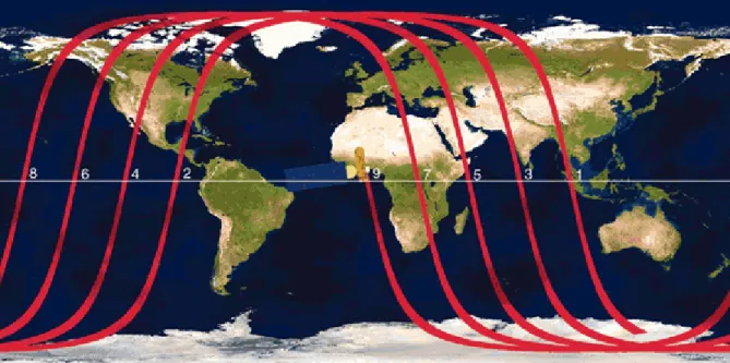
The Moderate Resolution Imaging Spectroradiometer (MODIS) instrument, on board of Earth Observing System (EOS) Terra (launched 18 December 1999) and Aqua (launched 4 May 2002) satellites, was designed to include characteristics specifically for fire detection. It has a sun-synchronous, near-polar, circular orbit, with a swath of 2330 km (cross track) by 10 km (along track at nadir) (Figure 1). With 36 spectral bands, the spatial resolution varies, being 250 m for bands 1-2, 500 m for bands 3-7 and 1000 m for bands 8-36 (Justice et al., 1998).
Figure 1 - Schematic of the Aqua orbit, with labels for nine consecutive passes over the equator (Parkinson, 1993)
There are two fire related products: MODIS Active-Fire Product and MODIS Burned Area Product. They provide information on the location of a fire, its emitted energy, the flamming and smoldering ratio, and an estimate of area burned. Fire observations are made four times a day from the Terra (10:30/22:30) and Aqua (13:30/01:30) satellites, and the detection is performed using a contextual algorithm that exploits the strong emission of mid-infrared radiation from fires (Justice et al., 2006; Giglio, 2010).
The algorithm examines each pixel of the MODIS swath, and ultimately assigns to each one of the following classes: missing data, cloud, water, non-fire, fire, or unknown. The algorithm uses essentially the difference between brightness temperatures derived from the MODIS 4 μm and 11 μm channels, the application of temperature thresholds, and the comparison with the brightness temperatures of neighbour pixels. The 12 μm channel is used for cloud masking. The 250 m resolution red and near-infrared channels, aggregated to 1 km, are
6 used to reject false alarms and mask clouds. The 500 m 2.1 μm band, also aggregated to 1 km, is used to reject water-induced false alarms (Giglio et al., 2003).
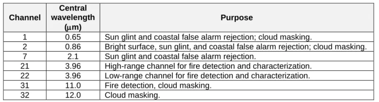
Table 1 resumes the MODIS channels used for active-fire detection.
Table 1 - MODIS channels used for active-fire detection and characterization (Justice et al., 2006)
Channel
Central wavelength
(m)
Purpose
1 0.65 Sun glint and coastal false alarm rejection; cloud masking.
2 0.86 Bright surface, sun glint, and coastal false alarm rejection; cloud masking. 7 2.1 Sun glint and coastal false alarm rejection.
21 3.96 High-range channel for fire detection and characterization. 22 3.96 Low-range channel for fire detection and characterization.
31 11.0 Fire detection, cloud masking.
32 12.0 Cloud masking.
For this work, the analysis period spanned from July 2002 to December 2009 (90 months, 7.5 years), the period for which there is information from both MODIS Terra and Aqua. The data was previously screened based on a product filtering, described by Mota et al. (2006) and Oom et al. (2008), with the objective of eliminating commission errors. This procedure consists of three phases: first, a series of spatial masks were used to classify false alarms and non-vegetation fires generated by specific types of land cover, gas flares, and volcanic activity; secondly, several spatial statistical techniques were applied as to detected space and time anomalies that may be associated with non-vegetation fires; finally, the data were visually analyzed to classify erroneous observations not detected in the other stages.
2.2. Climate data
For this study, data from the NOAA National Center for Environmental Prediction (NCEP), NCEP/NCAR Reanalysis monthly means (Kalnay et al., 1996), were used. Specifically, air temperature, relative humidity and precipitation water, with a spatial coverage of 2.5º 2.5º global grid, and for the period January 2000 to December 2009.
Two indexes from climate phenomena were also used:
- ENSO (El Niño-Southern Oscillation): Southern Oscillation Index (SOI), sea level pressure anomaly, from NOAA/Climate Prediction Center
(http://www.cpc.ncep.noaa.gov/data/indices/)
- IOD (Indian Ocean Dipole): Dipole Mode Index (DMI), SST DMI dataset derived from HadISST dataset, from JAMSTEC/FRCGC
7
3. METHODS
3.1. DETERMINATION OF DIFFERENT FIRE REGIMES PARAMETERS 3.1.1. Defining the study areas
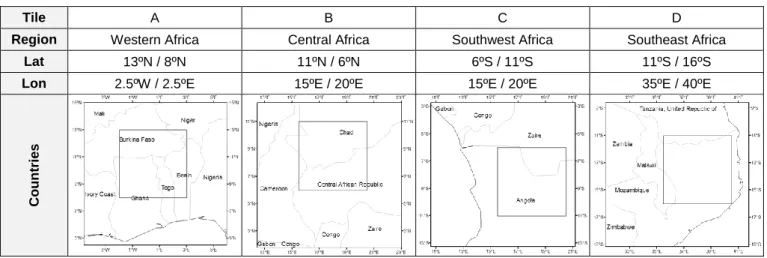
Having global information on fire counts, the first step was to extract fire counts time series for specific locations. The analysis was restricted to the African continent, since it is the one that burns the most and has very different fire behaviours all around (Dwyer et al., 1999; Carmona-Moreno et al., 2005; van der Werf et al., 2006, 2010). From this were established three regions: the totality of the continent (AFRICA), the north and the south hemispheric parts (AFRICA_NH, AFRICA_SH), given that fire regime is very different above and below the equator. Secondly, knowing that savannas, grasslands and shrublands are the cover types with more representative area, with high fire frequency, density burning and short fire-return interval (Dwyer et al., 1999, 2000; Silva et al., 2003; van der Werf et al., 2008), it was used the „Tropical and Subtropical Grasslands, Savannas and Shrublands‟ biome, taken from the „WWF Terrestrial Ecoregions of the World‟ (Olson et al., 2001), also divided by hemispheres (TSGSS_NH, TSGSS_SH, Figure 2). Finally, four spatial windows (Figure 3, Table 2), with an area of 5º 5º, were selected from this biome, in order to represent smaller regions.
Figure 2 – ‘Tropical and Subtropical Grasslands, Savannas and Shrublands’ biome (Olson et al., 2001), north and south hemispheric parts (TSGSS_NH, TSGSS_SH)
8
Figure 3 – Spatial representation of tiles A to D. Details in Table 2.
Table 2 – Spatial windows considered for the fire counts time series analysis.
Tile A B C D
Region Western Africa Central Africa Southwest Africa Southeast Africa
Lat 13ºN / 8ºN 11ºN / 6ºN 6ºS / 11ºS 11ºS / 16ºS
Lon 2.5ºW / 2.5ºE 15ºE / 20ºE 15ºE / 20ºE 35ºE / 40ºE
Coun
trie
s
3.1.2. Fire season length and peak month of fire activity
As to characterize the fire frequency in the study areas some parameters were explored for each of them (and individually for the Terra, Aqua and Terra + Aqua fire counts time series). A simple analysis of each series was made as to understand the start, peak, end and length of the fire season in each region. Following Giglio et al. (2006), the fire season duration is the number of months during which the average monthly fire counts is at least 10% of the average annual fire counts, and the peak month of fire activity is the calendar month during which the maximum number of average monthly fire counts was detected.
9
3.1.3. Diurnal fire cycle
Another aspect that was considered was the existence of a diurnal fire cycle. The Terra and Aqua satellites have orbits with local equatorial crossing times of 10.30/22.30 and 01.30/13.30, respectively, which offer the opportunity to examine different points of the diurnal fire cycle. A simple analysis of the fraction of the total fire counts (Terra + Aqua) detected by the Aqua satellite can give an idea of the magnitude of the difference between fires detected in the midmorning (Aqua, 10:30) and early afternoon (Terra, 13:30).
3.1.4. Interannual variability
To study the interannual variability of fire activity, a 12-month lagged autocorrelation was calculated for all series. According to Giglio et al. (2006, 2009), this provides a measure of interannual variability and periodicity of fire activity, where regions of high anthropogenic fire activity and low interannual rainfall variability should exhibit a very high temporal autocorrelation. Conversely, regions of low anthropogenic fire activity and high interannual rainfall variability should exhibit a very low temporal autocorrelation. Also, the correlation between the Terra and Aqua fire counts time series was considered to evaluate the consistency in seasonality, since it is sensitive to differences in the timing of fire activity (fire season length, location and number of peaks), but relatively insensitive to differences in the magnitude of the time series. The better the relationship, the most similar behaviour have the two series, or else, the more similar would be the seasonality of the two series.
3.2. APPLYING THE EMD METHOD TO THE FIRE COUNTS TIME SERIES 3.2.1. Empirical mode decomposition (EMD)
This topic is largely based on the publications Huang et al. (1998), Huang et al. (1999), Huang et al. (2003) and Huang & Wu (2008).
Huang et al. (1998) firstly introduced this new method of time series analysis. The authors presented it as an “intuitive, direct, a posteriori and adaptive method, with the basis of the decomposition based on, and derived from, the data” (Huang et al., 1998: pp. 917). The decomposition has implicitly a simple assumption that, at any given time, the data may have many coexisting simple oscillatory modes of significantly different frequencies, one superimposed on the other. Each of the modes is defined as an intrinsic mode function (IMF), satisfying two conditions:
10 (1) in the whole data set, the number of extrema and the number of zero crossings must
either equal or differ at most by one; and
(2) at any point, the mean value of the envelope defined by the local maxima and the envelope defined by the local minima is zero.
The decomposition of any function through the sifting process is meant to extract IMFs level by level, to identify the intrinsic oscillatory modes by their characteristic time scales in the data empirically, and then decompose the data accordingly. First, the IMF with the highest frequency, finest scale, shortest-period oscillation is extracted, then the next one from the difference between the data and the extracted IMF, and so on. The sifting process serves two purposes:
(1) to eliminate background waves on which the IMF is riding (2) to make the wave profiles more symmetric.
The procedure, starting with the data x(t) to be decomposed, can be resumed as follows: 1. Initialize: r0(t) = x(t), i = 1
2. Extract the ith IMF:
2.1. Initialize: h0(t) = ri-1(t), k = 1
2.2. Identify all the local extrema (maxima and minima) of hk-1(t)
2.3. Connect them to form the upper (emax(t)) and lower (emin(t)) envelopes
2.4. Calculate the mean: m(t) = [emax(t) + emin(t)]/2
2.5. Get the first component: hk(t) = hk-1(t) – m(t) 2.6. Check if hk(t) satisfies the definition of IMF.
i. If so: hk(t) = IMFi(t)
ii. If not: repeat the sifting as many times as required to make the extracted signal satisfy the condition of an IMF; k = k + 1, go to 2.2. 3. ri+1(t) = ri(t) – IMFi(t)
4. If the residue:
i. still contains longer-period variations, so it is treated as the new data and submitted to the same sifting process as to obtain a lower frequency IMF; i = i + 1, go to 2.
ii. becomes a monotonic function, or one with only one extreme from which no more IMFs can be extracted, the decomposition stops; the final ri+1(t) is the trend of x(t)
5. x(t) can be represented as:
x(t) = IMFi(t) + IMFi+1(t) + ... + IMFn(t) + ri+1(t), with n as the number of IMFs produced
11 This method has been applied widely. Huang & Shen (2005) discussed applications in various scientific fields, and Huang & Attoh-Okine (2005) discussed applications for engineering. Other works referred to series of global temperature (Zhen-Shan & Xian, 2007), climate anomalies (Wu et al., 2001, 2008; Salisbury & Wimbush, 2002), solar cycle and insolation (Coughlin & Tung, 2004a, 2004b; Lin and Wang, 2006), meteorological datasets (Duffy, 2004), crude oil price (Zhang et al., 2007, 2009), and so on.
3.2.2. Applying the EMD
Having the fire counts time series for each defined area characterized, the second part of the work consisted in apply the EMD method to them. Within the method terminology, these series are called „signal‟, that is, the original time series that will be decomposed.
For this was used an EMD algorithm available as an R package, created and maintain by Kim & Oh (2009a, 2009b). The function that performs empirical mode decomposition is
emd(), which has the following relevant arguments:
emd(xt, tt, max.sift=10, stoprule="type2", boundary="wave", max.imf=10)
where xt is the signal, tt the time index, max.sift the maximum number of sifting (100 steps was chosen to unsure that there was not an overshifting of the data, but there was significant space for the IMFs to appear), stoprule for the sifting process was defined as
type2 (the Cauchy like convergence criterion), boundary was set as wave (as was used by Huang et al. (1998)), and max.imf the maximum number of IMFs (left as 10, not having influence since there was always lesser IMFs produced; in the procedure explained before, the decomposition would stop if i > max.imf).
An observational analysis was made, as to try to discern the possible significance of each function in each set. It was followed by some algebraic manipulation of the functions, for example, extracting from the signal the IMF correspondent to the seasonality as to try and understand what other factors influence the time series besides the periodic behaviour of it, and so on.
3.3. RELATING THE IMF’S TO VARIABLES INFLUENCING FIRE
First, we tried to simply correlate precipitation, air temperature and relative humidity time series with the various IMFs obtained, experimenting with multiple lags. The same was done with the SOI and DMI indexes. Secondly, precipitation was accumulated for different time periods and related with the sum of fire occurrences in the fire season, as well as the sum of the intrinsic functions series values for the same period. A 24, 18 and 12-month accumulation of precipitation, prior to the fire season start, were used.
12
4. RESULTS AND DISCUSSION
4.1. DETERMINATION OF DIFFERENT FIRE REGIMES PARAMETERS 4.1.1. Fire season length and peak month of fire activity
Accounting for the 9 study areas, in which there will be three different fire counts series (for each of the satellites, Terra and Aqua series, and for the sum of all counts, Terra + Aqua series), there is a total of 27 monthly fire counts time series to study. The first batch of defined areas, related to the continent (AFRICA, AFRICA_NH and AFRICA_SH) are presented in Figure 4, where solid lines represent the Terra + Aqua series, dotted and dashed lines the Terra and Aqua series, respectively, for the period from July 2002 to December 2009. The same information in displayed in Figure 5 for the TSGSS_NH and TSGSS_SH, and in Figure 6 for each of the four tiles selected (Table 2).
Figure 4 – MODIS Terra/Aqua monthly fire counts time series for the totality of the African continent (first panel), and for the northern (second) and southern (third) parts.
Comparing the first panel of Figure 4 to the other two, it can be easily spotted that the African continent time series, with its two-peak fire activity, is a mix of two different fire behaviours, from the northern and the southern parts. Looking to Figure 5 as well, other simple evidence is the similitude of the fire counts time series of each part of the TSGSS biome when compared with the respective African northern and southern parts. Actually, TSGSS_NH fire counts represent 83.65% of the AFRICA_NH fire counts, and TSGSS_SH 83.33% of the AFRICA_SH. Since, as mentioned before, TSGSS is the most representative biome in Africa, and the one with more fire events, this was already expected.
AFRICA_NH AFRICA 0 100000 200000 300000 400000 0 100000 200000 300000 400000 0 100000 200000 300000 400000 AFRICA_SH Ju l-02 Oct -02 Ja n -03 A p r-03 Ju l-03 Oct -03 Ja n -04 A p r-04 Ju l-04 Oct -04 Ja n -05 A p r-05 Ju l-05 Oct -05 Ja n -06 A p r-06 Ju l-06 Oct -06 Ja n -07 A p r-07 Ju l-07 Oct -07 Ja n -08 A p r-08 Ju l-08 Oct -08 Ja n -09 A p r-09 Ju l-09 Oct -09
MODIS Terra/Aqua Fire Counts Series for AFRICA, AFRICA_NH and AFRICA_SH
13
Figure 5 – MODIS Terra/Aqua monthly fire counts time series for the TSGSS biome northern (first panel) and southern (second) parts.
Table 3 – TSGSS fire season calendar ( fire season, peak month)
Area Series Months Season
length J F M A M J J A S O N D TSGSS_NH T+A 8 T 7 A 8 TSGSS_SH T+A 7 T 7 A 6
For the African continent and TSGSS biome, there are two distinct behaviours depending on the hemispheric part in evaluation. As already reported, the onset of the dry season highly changes between northern and southern Africa, being associated with it two very different fire seasons. In the north, as can be seen in Table 3 for TSGSS_NH, and later in Table 4 for tiles A and B, fire season starts in October and ends around April, with December/January as peak months of fire activity. As for the south, TSGSS_SH in Table 3, the fire season stretches from May through November. Here, there‟s another observation to be made: the fire season also varies from west to the east of Africa, settling first in the west (tile C in Table 4) around April/May, and later in the east (tile D in Table 4) on May/June. It then ends in September and November, having peak months in July and September, respectively. This temporal pattern of fire activity in Africa is in line with previous works.
TSGSS_SH TSGSS_NH 0 100000 200000 300000 400000 0 100000 200000 300000 400000 Ju l-02 Oct -02 Ja n -03 A p r-03 Ju l-03 Oct -03 Ja n -04 A p r-04 Ju l-04 Oct -04 Ja n -05 A p r-05 Ju l-05 Oct -05 Ja n -06 A p r-06 Ju l-06 Oct -06 Ja n -07 A p r-07 Ju l-07 Oct -07 Ja n -08 A p r-08 Ju l-08 Oct -08 Ja n -09 A p r-09 Ju l-09 Oct -09
MODIS Terra/Aqua Fire Counts Series for the TSGSS_NH and TSGSS_SH
14
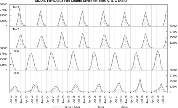
Figure 6 – MODIS Terra/Aqua monthly fire counts time series for the tiles A, B, C and D (first, second, third and fourth panel, respectively).
Table 4 – Tiles A to D fire season calendar ( fire season, peak month)
Tile Series Months Season
length J F M A M J J A S O N D A T+A 6 T 5 A 6 B T+A 6 T 7 A 6 C T+A 5 T 6 A 5 D T+A 7 T 6 A 7
4.1.2. Diurnal fire cycle
By discriminating Terra and Aqua fire counts time series, other aspects of the fire behaviour can be studied. Terra captures much lesser fire events than Aqua, making the passing time of the satellites in these areas a key factor for the study of fire activity, allowing the examination of different points of the diurnal fire cycle. Actually, the fraction of all fire counts (Terra + Aqua) observed by the Aqua satellite (Table 5) rounds 70%, with higher percentages for the southern parts of Africa, making its passing time probably more nearer the peak of daily fire activity than the Terra passing time.
0 12500 25000 37500 50000 0 12500 25000 37500 50000 Tile D Tile C Tile B Tile A 0 12500 25000 37500 50000 0 12500 25000 37500 50000 Ju l-02 O c t-02 Ja n -03 A p r-03 Ju l-03 O c t-03 Ja n -04 A p r-04 Ju l-04 O c t-04 Ja n -05 A p r-05 Ju l-05 O c t-05 Ja n -06 A p r-06 Ju l-06 O c t-06 Ja n -07 A p r-07 Ju l-07 O c t-07 Ja n -08 A p r-08 Ju l-08 O c t-08 Ja n -09 A p r-09 Ju l-09 O c t-09
MODIS Terra/Aqua Fire Counts Series for Tiles A, B, C and D
15 Various authors already had mentioned the possible existence of this cycle, like Langaas (1993), Eva and Lambin (1998b) and Giglio et al. (2006). Pack et al. (2000) and particularly Giglio (2007) studied this cycle, and arrived to the conclusion that the peak of fire activity in this region occurs in the afternoon, around 2 p.m. local time. As Aqua satellite passing time is 13:30/01:30, against Terra‟s 10:30/22:20, it is natural that the MODIS sensor aboard of Aqua satellite captures much more fire occurrences then Terra‟s MODIS sensor.
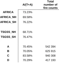
Table 5 - Percentage of the total fire counts observed only by Aqua satellite MODIS sensor.
A/(T+A) Total number of fire counts AFRICA 73.23% AFRICA_NH 69.58% AFRICA_SH 76.22% TSGSS_NH 68.71% TSGSS_SH 76.47% A 70.45% 542 394 B 70.05% 625 915 C 83.58% 940 308 D 70.29% 417 193 4.1.3. Interannual variability
When applying 12-month autocorrelations, to study year-to-year variability, to the 27 fire counts fire series, the lower values of autocorrelation obtained (Figure 8) were for AFRICA Tile A, and Tile D. In general, Terra time series have slightly lower values than the Aqua time series. Even so, all values were above 0.743. This makes this a continent with very little interannual variation in its fire activity.
As for the correlations between Terra and Aqua time series (summary of all correlations in Figure 9, and individual plots of the series in Figure 7), all were above 0.9176, except AFRICA with 0.6923, making them consistent with each other.
16 MOD IS A q u a f ire c o u n ts s e rie s ( 10 3 )
MODIS Terra fire counts series ( 103)
Figure 7 – MODIS Terra (x-axis) versus Aqua (y-axis) fire counts time series, with linear relation represented
y = 2,1476x + 31685 R² = 0,6923 0 100 200 300 0 100 200 300 AFRICA y = 2,157x + 3596,9 R² = 0,9689 0 100 200 300 0 100 200 300 AFRICA_NH y = 3,2734x - 1805,6 R² = 0,9193 0 100 200 300 0 100 200 300 AFRICA_SH y = 2,1649x + 738,55 R² = 0,9702 0 100 200 300 0 100 200 300 TSGSS_NH y = 3,3808x - 2843,1 R² = 0,9176 0 100 200 300 0 100 200 300 TSGSS_SH y = 2,416x - 57,597 R² = 0,9673 0 10 20 30 0 10 20 30 Tile A y = 2,429x - 187,05 R² = 0,9767 0 10 20 30 0 10 20 30 Tile B y = 4,6357x + 782,27 R² = 0,9509 0 10 20 30 40 0 10 20 30 40 Tile C y = 2,419x - 72,714 R² = 0,9445 0 10 20 30 0 10 20 30 Tile D
17
Figure 8 – The 12-month autocorrelation values for each area and series.
Figure 9 – Correlations between Terra and Aqua time series, values for all areas (individual plots in Figure 7).
4.2. APPLYING THE EMD METHOD TO THE FIRE COUNTS TIME SERIES
Using the EMD package from R, the method was applied to all series, resulting in various IMFs sets for each one. In Table 6 is listed the number of IMF‟s produced for each series. There is also a residue per set. Furthermore, the datasets represented in the following figures are highlighted in the table for easier understanding.
Table 6 – Number of IMFs produced by applying EMD to each of the series
T+A Terra Aqua
AFRICA 4 4 4 AFRICA_NH 4 4 4 Figure 10 AFRICA_SH 4 4 4 TSGSS_NH 2 3 2 TSGSS_SH 3 3 3 Figure 11 A 2 4 2 B 4 4 4 Figure 12 C 4 4 3 D 4 4 5
Most of the series originated four IMFs (and a residue). Represented next are the datasets for the AFRICA_NH, TSGSS_SH and Tile B (located in central Africa, northern hemisphere) fire counts monthly time series EMD outputs. These series, now called the signals for each dataset, were plotted earlier in the second panel of Figure 4, Figure 5 and Figure 6, respectively. These were chosen because they all have the same number of IMFs, making it possible to compare the modes originated by the Terra and Aqua individual time series.
0,7 0,75 0,8 0,85 0,9 A FR IC A A FR IC A _ N H A FR IC A _ S H TS GSS _ N H TS GSS _ S H Til e A Til e B Til e C Til e D
12-Month Lagged Autocorrelation
Terra + Aqua Terra Aqua 0,832 0,984 0,959 0,985 0,958 0,984 0,988 0,975 0,972 0,8 0,85 0,9 0,95 1 A FR IC A A FR IC A _ N H A FR IC A _ S H TS GSS _ N H TS GSS _ S H Til e A Til e B Til e C Til e D Correlation
18
Figure 10 – MODIS Terra/Aqua fire counts monthly time series EMD output for AFRICA_NH.
Table 7 – Percentages of variance explain by each IMF and residue, and correlations of each mode with the signal, for AFRICA_NH EMD dataset.
% Variance of the signal % Variance of the dataset (IMFs + residue)
Correlation with the signal T+A T A T+A T A T+A T A IMF 1 28,21 % 30,25 % 26,69 % 19,03 % 22,58 % 19,41 % 0,18 0,24 0,16 IMF 2 114,45 % 102,88 % 117,96 % 77,20 % 76,81 % 77,13 % 0,84 0,85 0,84 IMF 3 3,84 % 0,55 % 3,57 % 2,59 % 0,41 % 2,34 % - 0,02 0,04 - 0,01 IMF 4 0,53 % 0,25 % 0,55 % 0,36 % 0,19 % 0,36 % 0,04 0,03 0,04 Residue 1,22 % 0,02 % 1,17 % 0,83 % 0,01 % 0,77 % 0,00 0,01 0,00 Total 148,25 % 133,95 % 152,94 % 100,00 % 100,00 % 100,00 %
For the AFRICA_NH EMD output dataset (Figure 10), IMF 2 clearly represents the annual cycle, the seasonality, accounting for more than 70% of the total variance, and with a correlation of 0,84 with the signal (Table 7). The amplitude of this IMF is larger for the Aqua than for the Terra time series. The next IMF that contributes most for the total variance is the IMF 1, associated with noise. IMF 3, 4 and the residue all have very low correlations with the signal, and low percentages of explained variance, showing that these functions contribute very little to the signal.
-15000 -7500 0 7500 15000 -60000 -30000 0 30000 60000 -200000 -100000 0 100000 200000 RES IMF 4 IMF 3 IMF 2 IMF 1 20000 45000 70000 95000 120000 -130000 -65000 0 65000 130000 Ju l-02 Oct -02 Ja n -03 A p r-03 Ju l-03 Oct -03 Ja n -04 A p r-04 Ju l-04 Oct -04 Ja n -05 A p r-05 Ju l-05 Oct -05 Ja n -06 A p r-06 Ju l-06 Oct -06 Ja n -07 A p r-07 Ju l-07 Oct -07 Ja n -08 A p r-08 Ju l-08 Oct -08 Ja n -09 A p r-09 Ju l-09 Oct -09
EMD output for the MODIS Terra/Aqua fire counts series for AFRICA_NH
19
Figure 11 – MODIS Terra/Aqua fire counts monthly time series EMD output for TSGSS_SH.
Table 8 – Percentages of variance explain by each IMF and residue, and correlations of each mode with the signal, for TSGSS_SH EMD dataset.
% Variance of the signal % Variance of the dataset (IMFs + residue)
Correlation with the signal
T+A T A T+A T A T+A T A
IMF 1 16,03 % 13,81 % 17,54 % 13,86 % 11,59 % 14,84 % 0,36 0,28 0,35
IMF 2 95,21 % 98,64 % 96,39 % 82,28% 82,78 % 81,58 % 0,88 0,90 0,88
IMF 3 1,00 % 6,51 % 1,01 % 0,87 % 5,47 % 0.86 % - 0,03 0,01 - 0,03
Residue 3,47 % 0,20 % 3,22 % 3,00 % 0,17 % 2,72 % - 0,02 - 0,03 - 0,03
Total 115,72% 119,16 % 118,16 % 100,00 % 100,00% 100,00%
In the dataset for TSGSS_SH (Figure 11), similar comments can be made. Again, IMF 2 represents an annual cycle, most probably related with seasonality, accounting for more than 80% of the total variance (Table 8), and IMF 1 related with noise. This first function starts with smaller amplitude that increases and stabilizes in the middle years (2004-07), increasing even more at the end. This has to be approached carefully: because of some end effects problems associated with this method, the boundary type selection can have some influence in the beginning and ending of the modes, not truly associated with intrinsic properties of the signal. IMF 3 and the residue have little significance in the set, with very low negative correlations with the signal.
-25000 -13750 -2500 8750 20000 -160000 -77500 5000 87500 170000 RES IMF 3 IMF 2 IMF 1 10000 40000 70000 100000 130000 -100000 -50000 0 50000 100000 Ju l-02 Oct -02 Ja n -03 A p r-03 Ju l-03 Oct -03 Ja n -04 A p r-04 Ju l-04 Oct -04 Ja n-05 A p r-05 Ju l-05 Oct -05 Ja n -06 A p r-06 Ju l-06 Oct -06 Ja n -07 A p r-07 Ju l-07 Oct -07 Ja n -08 A p r-08 Ju l-08 Oct -08 Ja n -09 A p r-09 Ju l-09 Oct -09
EMD output for the MODIS Terra/Aqua fire counts series of TSGSS_SH
20
Figure 12 – MODIS Terra/Aqua fire counts monthly time series EMD output for Tile B.
Table 9 – Percentages of variance explain by each IMF and residue, and correlations of each mode with the signal, for TSGSS_SH EMD dataset.
% Variance of the signal % Variance of the dataset (IMFs + residue)
Correlation with the signal
T+A T A T+A T A T+A T A
IMF 1 41,73 % 36,83 % 43,43 % 26,83 % 25,54 % 26,99% 0,22 0,24 0,21 IMF 2 113,38 % 106,69 % 116,78 % 72,87 % 73,99 % 72,57 % 0,81 0,82 0,80 IMF 3 0,34 % 0,56 % 0,33 % 0,22 % 0,39 % 0,21 % 0,01 0,03 - 0,03 IMF 4 0,09 % 0,09 % 0,20 % 0,06 % 0,06 % 0,12 % 0,01 0,01 0,00 Residue 0,03 % 0,02 % 0,17 % 0,02 % 0,02 % 0,11 % 0,01 0,05 - 0,03 Total 155,58 % 144,19 % 160,92 % 100,00 % 100,00 % 100,00 %
As for tile B EMD dataset, the same things can be said. As AFRICA_NH (where tile B is located), four IMFs were obtained. Of special attention is the very regular behaviour of the seasonal mode (IMF 2), that has the same seasonal pattern as AFRICA_NH (with peaks around December/January), and the residue that is almost constant (not showing any particular trend for this area). In addition, both IMFs 4 are similar, but IMF 3 has somewhat of an inverse appearance: with bigger waves at the end of the time period for AFRICA_NH, where in tile B the bigger waves are in the beginning, slowly decreasing in amplitude.
-800 -400 0 400 800 -1500 -750 0 750 1500 -20000 -10000 0 10000 20000 RES IMF 4 IMF 3 IMF 2 IMF 1 1000 2500 4000 5500 7000 -15000 -7500 0 7500 15000 Ju l-02 Oct -02 Ja n -03 A p r-03 Ju l-03 Oct -03 Ja n -04 A p r-04 Ju l-04 Oct -04 Ja n-05 A p r-05 Ju l-05 Oct -05 Ja n -06 A p r-06 Ju l-06 Oct -06 Ja n -07 A p r-07 Ju l-07 Oct -07 Ja n -08 A p r-08 Ju l-08 Oct -08 Ja n -09 A p r-09 Ju l-09 Oct -09
EMD output for the MODIS Terra/Aqua fire counts series for Tile B
21
Figure 13 – MODIS Terra + Aqua fire counts monthly time series EMD outputs for AFRICA (solid lines) and the sum between AFRICA_NH and AFRICA_SH individual IMFs (dashed lines).
Some arithmetic operations can be made between the IMFs obtained. In Figure 13 is a comparison between the IMFs of the AFRICA EMD output and the sum of the individual IMFs obtained for AFRICA_NH and AFRICA_SH, that is, AFRICA_NH IMF 1 + AFRICA_SH IMF 1, and so on. Given that the sum of all the IMFs plus the residue gives us the original signal, and since the AFRICA series is a sum of the NH and SH parts series, mathematically, the sum of the IMFs of the NH and SH should result in the original AFRICA signal. That is true. Only, the sum of each IMF does not equal the correspondent IMF of the AFRICA dataset, as can be noted in Figure 13.
Another option, taken into account in the next section, was to take from the signal the IMF correspondent to the seasonality, to examine only the perturbations to the signal. An example for Tile D series is plotted in Figure 14.
-40000 -22500 -5000 12500 30000 -80000 -40000 0 40000 80000 -170000 -90000 -10000 70000 150000 RES IMF 4 IMF 3 IMF 2 IMF 1 190000 202500 215000 227500 240000 -170000 -70000 30000 130000 230000 Ju l-02 Oct -02 Ja n -03 A p r-03 Ju l-03 Oct -03 Ja n -04 A p r-04 Ju l-04 Oct -04 Ja n -05 A p r-05 Ju l-05 Oct -05 Ja n -06 A p r-06 Ju l-06 Oct -06 Ja n -07 A p r-07 Ju l-07 Oct -07 Ja n -08 A p r-08 Ju l-08 Oct -08 Ja n -09 A p r-09 Ju l-09 Oct -09
EMD output for the MODIS T + A fire counts series for AFRICA and AFRICA_NH + AFRICA_SH
22
Figure 14 – Deseasonalisation of Tile D fire counts time series, by subtracting to the signal the corresponding IMF 2
4.3. RELATING THE IMF’S TO VARIABLES INFLUENCING FIRE
The best correlation value obtained between the Southern Oscillation Index, the Dipole Mode Index and all the IMFs produced earlier, was between the SOI (Figure 15a) and the second IMF from the TSGSS_NH EMD output (Figure 15b). For a 10-month lag applied to the SOI series, a cross-correlation value of -0.522 was obtained (Figure 15c). The two series (the IMF 2 and the lagged and inverted SOI) are represented in Figure 15d, Although there seems to be a relation between them, when analysing the importance of this IMF 2 for the TSGSS_NH (T+A) signal (Table 10), the contribution is very low. If accounts for less than 1% of the variance, with a very low correlation with the signal (-0.01).
a) b)
c) d)
Figure 15 – Relation between the Southern Oscillation Index (SOI) and the IMF 2 of TSGSS_NH: SOI series for the study period (a); the second IMF from the TSGSS_NH EMD output (b); the cross-correlations values for the two series for several lags (c); overlap between the two series, constrained to [0, 1], with SOI represented horizontally inverted (for ease of comprehension, since the correlation had a negative value) and with a 10-month lag (d).
-10000 0 10000 20000 30000 40000 Ju l-02 Ou t-02 Ja n -03 A b r-03 Ju l-03 Ou t-03 Ja n -04 A b r-04 Ju l-04 Ou t-04 Ja n -05 A b r-05 Ju l-05 Ou t-05 Ja n -06 A b r-06 Ju l-06 Ou t-06 Ja n -07 A b r-07 Ju l-07 Ou t-07 Ja n -08 A b r-08 Ju l-08 Ou t-08 Ja n -09 A b r-09 Ju l-09 Ou t-09
Tile D fire counts time series: original signal and signal deseasonalised
Signal Signal - IMF 2
-8 -4 0 4 8 Ju l-02 Dec -02 M ay -03 Oct -03 M a r-04 A u g -04 Ja n -05 Ju n -05 Nov -05 A p r-06 S e p -06 F e b -07 Ju l-07 Dec -07 M ay -08 Oct -08 M a r-09 A u g -09
Southern Oscillation Index (SOI)
-15000 -10000 -50000 5000 10000 15000 Ju l-02 Dec -02 M ay -03 Oct -03 M a r-04 A u g -04 Ja n -05 Ju n -05 Nov -05 A p r-06 S e p -06 F e b -07 Ju l-07 Dec -07 M ay -08 Oct -08 M a r-09 A u g -09 TSGSS_NH: IMF 2 -15 -10 -5 0 5 10 15 -0 .4 -0 .2 0 .0 0 .2 Lag A C F SOI & TN_2 0 0,2 0,4 0,6 0,8 1 TSGSS_NH: IMF 2 SOI [x+10]
23
Table 10 – Percentages of variance explain by each IMF and residue, and correlations of each mode with the signal, for TSGSS_NH (T+A) EMD dataset.
% Var. of the signal % Var. of the dataset (IMFs + residue)
Correlation with the signal IMF 1 100,52 % 98,05 % 1,00 IMF 2 0,55 % 0,53 % - 0,01 IMF 3 0,77 % 0,75 % 0,02 Residue 0,68 % 0,67 % 0,01 Total 102,52 % 100,00 %
24
5. CONCLUSION
In view of the fact that no relevant results have been obtained, some considerations are made relatively to the method itself and its application to this type of time series:
i. Empirical mode decomposition is a very recent method in the analysis of time series. Since 1998, it has been suffering many improvements and developments (Huang and Wu, 2008). But still, many of them remain in the theoretical field, and there‟s a lack of user-oriented software applications. Of my knowledge, there‟s only available a packaged for R [Kim and Oh, 2009], with limited functions, and another for MATLAB made by Zhaohua Wu, one of the authors, and also dealing with limited options. Many of the more recent studies deal with many mathematical subtleties, in a language hard to follow by more lay people, as myself. This makes it hard to autonomously implement the method fully.
ii. Also, because of its youth, it is still a technique in need of further exploration, mainly due to the several parameters passive of being manipulated. As Huang et al. (2003: pp. 2319) puts it “There are many possible selections of free parameters, such as the maximum number of sifting times and the stopping criteria for extracting each intrinsic mode function (IMF). Each of the parameters can be selected independently of the others, and there are few, if any, solid guidelines to follow in the selection of these parameters. The obvious (yet critical) question is which set of the many possible choices of sifting parameters gives a meaningful result. This also leads to further questions: how can the goodness or the reliability of any result be measured?” This can make the method very variable.
iii. With new findings, always comes a new reality, and many times there‟s not a mental instrumentation to readily keep up with it. Concerning the interpretation of the outputs generated, we are looking at them through knowledge we already have, trying to find events and relationships that we already know about. But actually, the potential of this technique resides in the fact that it doesn‟t rely on a priory knowledge, but instead, gives us only the intrinsic properties of the signal. So, what is probably happening is that much of the information that is given in the form of IMFs isn‟t actually uncovered, information that we are still unable to fully comprehend.
iv. To work, EMD needs complete, continuous, series. This can arise as another possible answer to the lack of results. Any global fire product only represents a
25 fraction of the total fires which actually take place. This is due to bias related with low revisit frequencies by the satellites (detecting only a fraction of the fires, given that they usually last only a few hours), nonoptimal overpass time (related with the existence of a diurnal fire cycle), coarse spatial resolution, atmospheric opacity, false alarms, and intrinsic differences in Terra and Aqua MODIS instruments (Eva and Lambin, 1998a, 1998b; Giglio et al., 1999, 2003, 2006, 2007; Mota et al., 2006; Oom et al., 2008). For these reasons, the fire counts time series used are not full series of all the fire events that occurred for a specific region over the study period, thus making them somewhat of incomplete, and not true representations of the actual continuous fire. As a result, when applying the method, we are getting IMFs related with only part of the real fire counts series. This may signify that they will not have a real physical meaning.
v. Ignoring the previous constrain, and assuming that even with the current fire series relevant IMFs are obtained, other limitations come up. Fire is influenced by numerous factors, already described in the introduction. Precipitation, temperature, relative humidity, wind, topography, vegetation, herbivores, humans... the list of influencing variables over fire is endless. And these don‟t even represent isolated variables: they all interact with each other, and those interactions don‟t always work in a regular fashion, making it truly impossible to discern what influences, when, where and how. As such, assuming that a single IMF could correspond to a specific factor, demonstrating its individual contribution for the number of fire occurrences, seems quite improbable. Furthermore, trying to discover what mixture of variables behaviours are masked in each intrinsic function turns this into a much more complex problem. More, even, when we consider that there is not a very large consensus in the scientific community relatively to what the main influencing variables are, and how they act on fire. This would need a more in-depth multivariate statistical analysis.
vi. If, again, we do not consider the previous problem, there‟s also something to say about the climatic variables used in this study. The study period, which spanned from July 2002 to December 2009, does not include any strong climatic event, not ENSO or IOD. So, these would not exert any particular influence in the climate that would translate in a significant change in fire behaviour. Also, precipitation, temperature and relative humidity, all had low interannual variations, again, showing that this time period didn‟t had any remarkable event.
26 vii. As till today, no application of EMD to fire related series has been made, or at least, to my knowledge. This work became somewhat of a blind, but interesting, journey to what concerns the EMD application and output comprehension, making the discussion limited due to the lack of comparable studies. Of course, there are various applications of EMD on other fields, and some extrapolations can be made, but nothing to do with the interpretation of the IMFs meaning. Also, on a personal note, just my co-supervisor was familiarized with the more specific aspects of this technique, but not with the most recent developments, so, I was limited as to the people I could reach to when having more technical problems.
Even so, in the future, some possibilities may be considered, as:
- Instead of satellite derived fire information, maybe use some fire information derived from regional monitoring, possibly in a daily time step, which would be more accurate as to the fraction of fire events counted.
- Trying to make this analysis for other region, perhaps Australia, since Africa is known for its very regular fire behaviour, with low interannual variability, showing that it doesn‟t suffer many alterations from external variables to that seasonality.
- Something interesting would be to apply some of the most recent developments, for example, use the image analysis version of EMD, as to try and find some sort of geographical patterns of disturbance.
27
BIBLIOGRAPHY
Archibald, S., Roy, D.P., van Wilgren, B.W., Scholes, R.J. (2008) What limits fire? An examination of drivers of burnt area in Southern Africa. Global Change Biology 15(3): 613-630
Archibald, S., Kirton, A., Scholes, R.J., Schulze, R. (2010a) Defining an appropriate measure of accumulated rainfall to estimate fuel loads and derive burnt area. in Archibald, S. Fire Regimes
in Southern Africa - Determinants, Drivers and Feedbacks. PhD thesis. University of the
Witwatersrand
Archibald, S., Nickless, A., Govender, N., Scholes, R.J., Lehsten, V. (2010b) Climate and the inter-annual variability of fire in southern Africa: a meta-analysis using long-term field data and satellite-derived burnt area data. Global Ecology and Biogeography 19(6): 794-809
Archibald, S., Scholes, R.J., Roy, D.P., Roberts, G., Boschetti, L. (2010c) Southern African fire regimes as revealed by remote sensing. International Journal of Wildland Fire 19(7): 861-878 Barbosa, P.M., Stroppiana, D., Grégoire, J.-M., Pereira, J.M.C. (1999) An assessment of vegetation
fire in Africa (1981–1991): Burned areas, burned biomass, and atmospheric emissions. Global
Biogeochemical Cycles 13(4): 933-950
Bond, W.J., Woodward, F.I., Midgley, G.F. (2005) The global distribution of ecosystems in a world without fire. New Phytologist 165: 525-538
Bowman, D.M.J.S., Balch, J.K., Artaxo, P., Bond, W.J., Carlson, J.M., Cochrane, M.A., D‟Antonio, C.M., DeFries, R.S., Doyle, J.C., Harrison, S.P., Johnston, F.H., Keeley, J.E., Krawchuk, M.A., Kull, C.A., Marston, J.B., Moritz, M.A., Prentice, C., Roos, C.I., Scott, A.C., Swatnam, T.W., van der Werf, G.R., Pyne, S.J. (2009) Fire in the Earth system. Science 324, 481–484
Carmona-Moreno, C., Belward, A., Malingreau, J.-P., Hartley,A., Garcia-Alegre, M., Antonovskiy, M., Buchshtaber, V., Pivovarov, V. (2005) Characterizing interannual variations in global fire calendar using data from Earth observing satellites. Global Change Biology 11: 1537–1555 Cahoon, D.R., Stocks, B.J., Levine, J.S., Cofer, W.R., O‟Neill, K.P. (1992) Seasonal distribution of
African savanna fires. Nature 359(6398): 812-815
Coughlin, K., Tung, K.K. (2004a) Eleven-year solar cycle signal throughout the lower atmosphere.
Journal of Geophysical Research 109
Coughlin, K.T., Tung, K.K. (2004b) 11-Year solar cycle in the stratosphere extracted by the empirical mode decomposition method. Advances in Space Research 34:323–329
Duffy, D.G. (2004) The Application of Hilbert–Huang Transforms to Meteorological Datasets. Journal
of Atmospheric and Oceanic Technology 21: 599-611
Dwyer, E., Pereira, J.M.C., Grégoire, J.-M., DaCamara, C.C. (1999) Characterization of the spatio-temporal patterns of global fire activity using satellite imagery for the period April 1992 to March 1993. Journal of Biogeography 27: 57–69
28
Dwyer, E., Pinnock, S., Grégoire, J.-M., Pereira, J.M.C. (2000) Global spatial and temporal distributions of vegetation fire as determined from satellite observations. International Journal of
Remote Sensing 21(6 & 7): 1289-1302
Eva, H., Lambin, E.F. (1998a) Burnt area mapping in Central Africa using ATSR data. International
Journal of Remote Sensing 18: 3473-3497
Eva, H., Lambin, E.F. (1998b) Remote sensing of biomass burning in tropical regions: sampling issues and multisensory approach. Remote Sensing of Environment 64: 292-315
Flannigan, M.D., Krawchuk, M.A., de Groot, W.J., Wotton, B.M., Gowman, L.M. (2009) Implications of changing climate for global wildland fire. International Journal of Wildland Fire 18: 483–507 Giglio, L., Descloitres, J., Justice, C.O., Kaufman, Y.J. (2003) An Enhanced Contextual Fire Detection
Algorithm for MODIS. Remote Sensing of Environment 87: 273-282
Giglio, L., Csiszar, I., Justice, C.O. (2006) Global distribution and seasonality of active fires as observed with the Terra and Aqua Moderate Resolution Imaging Spectroradiometer (MODIS) sensors. Journal of Geophysical Research 111, G02016
Giglio, L. (2007) Characterization of the tropical diurnal fire cycle using VIRS and MODIS observations. Remote Sensing of Environment 108: 407-421
Giglio, L. (2010) MODIS Collection 5 Active Fire Product User's Guide Version 2.4
Huang, N.E., Shen, Z., Long, S.R., Wu, M.C., Zheng, Q., Yen, N., Tung, C.C., Liu, H.H. (1998) The empirical mode decomposition and the Hilbert spectrum for nonlinear and non-stationary time series analysis. Proc. R. Soc. Lond. A 454(1971): 903-995
Huang, N.E., Shen, Z., Long, S.R. (1999) A new view of nonlinear water waves: The Hilbert Spectrum.
Annual Review of Fluid Mechanics 31: 417-457
Huang, N.E., Wu, M.-L.C., Long, S.R., Shen, S.S.P., Qu, W., Gloersen, P., Fan, K.L. (2003) A confidence limit for the empirical mode decomposition and Hilbert spectral analysis. Proc. R.
Soc. Lond. A 459: 2317-2345
Huang, N.E., Attoh-Okine, N.O. (eds) (2005) The Hilbert-Huang Transform in Engineering. CRC Taylor & Francis
Huang, N.E., Shen, S.S.P. (eds) (2005) Hilbert-Huang Transform and its applications. World Scientific Huang, N.E., Wu, Z. (2008) A review on the Hilbert-Huang transform: method and its applications to
geophysical studies. Reviews of Geophysics 46
Justice, C.O., Vermote, E., Townshend, J.R.G., Defries, R., Roy, D.P., Hall, D.K., Salomonson, V.V., Privette, J.L., Rigss, G., Strahler, A., Lucht, W., Myneni, R.B., Knyazikhin, Y., Running, S.W., Nemani, R.R., Wan, Z., Huete, A.R., van Leeuwen, W., Wolfe, R.E., Giglio, L., Muller, J.-P., Lewis, P., Barnsley, M.J. (1998) The Moderate Resolution Imaging Spectroradiometer (MODIS):