FACULDADE DE
ENGENHARIA DA
UNIVERSIDADE DO
PORTO
A MapReduce Construct for Yap Prolog
Joana Côrte-Real
Mestrado Integrado em Engenharia Eletrotécnica e de Computadores Supervisors: Prof. Inês Dutra and Prof. Ricardo Rocha
c
Resumo
Neste trabalho, desenhou-se e implementou-se uma primitiva de alto nível para Prolog, baseada no paradigma de programação MapReduce. MapReduce é um modelo de programação funcional popularizado pela Google em 2008, apesar de ter raizes consideravelmente mais antigas. Este modelo é constituído por duas operações simples, map e reduce, que podem ser facilmente apli-cadas a um vasto número de algoritmos. Prolog, por sua vez, é uma linguagem assente em lógica de predicados de primeira ordem, com elevado poder declarativo, o que permite ao programador focar-se no algoritmo de resolução de um dado problema em vez de nos seus detalhes de mais baixo nível. Prolog é um modelo de programação vocacionado para o armazenamento e trata-mento de dados, havendo mesmo aplicações que estão preparadas para fazer inferências sobre esses dados. Um construtor MapReduce aplicado neste cenário permitiria escalar eficientemente todo o processo, reduzindo muito significativamente o tempo de execução.
A criação de uma primitiva de programação baseada em MapReduce para Prolog apresenta três contribuições principais: (i) proporciona ao utilizador uma construção de alto nível de ab-stração no modelo funcional MapReduce, mantendo a característica declarativa dos programas; (ii) disponibiliza ao utilizador uma construção não existente em Prolog e que é representativa de aplicações em várias áreas; (iii) permite paralelização, acelerando a execução de programas que utilizam esta primitiva. Este último ponto é particularmente relevante dado que os processadores de vários núcleos se têm tornado a escolha dominante em equipamentos informáticos, mesmo aqueles destinados a uso pessoal. Este facto, aliado à crescente quantidade de dados que, cada vez mais, são produzidos diariamente, faz com que uma ferramenta que utilize arquiteturas multi-processador – eficientemente – para processamento de dados, suscite interesse.
O foco de MapReduce para Prolog são as arquiteturas multi-processador, apesar de a nossa primitiva estar preparada para suportar ambientes híbridos (memória distribuída e memória partil-hada), de forma implícita e transparente para o utilizador. MapReduce para Prolog foi implemen-tado no sistema Yap e é constituído por uma arquitetura do tipo mestre-escravo, onde o mestre é responsável pela divisão do trabalho e os escravos pelo processamento das tarefas que lhes são atribuídas. A interface do construtor dispõe ainda de vários níveis de customização, e um dos objetivos deste trabalho é a integração do nosso contrutor MapReduce com o sistema Yap sob a forma de uma biblioteca. O nosso sistema foi testado com sucesso através da construção de quatro aplicações distintas comuns na literatura: duas contendo dados numéricos, e as restantes contendo termos de Prolog. Os testes foram feitos com duas implementações para a mesma interface de programação, uma para um cluster de máquinas e outra para uma arquitetura multi-processador. Determinou-se que o construtor escalou consistentemente o tempo de execução de forma quase ideal para todas as aplicações, quer em memória partilhada, quer distribuída. Desenvolveram-se e analisaram-se quatro técnicas de escalonamento de trabalho, das quais as mais eficazes serão disponibilizadas na versão final da biblioteca. Finalmente, avaliou-se ainda o efeito da variação do tamanho das unidades de trabalho distribuídas aos escravos a fim de establecer os parâmetros por defeito para MapReduce para Prolog.
Abstract
This work’s aim was to design and implement a high-level Prolog primitive, based on the MapRe-duce programming paradigm. MapReMapRe-duce is a programming model made popular by Google in 2008, even though its origins are more remote. It is composed by two simple operations, map and reduce, which can easily be applied to numerous algorithms. On the other hand, Prolog is a first-order logic predicate language with significant declarative power. This allowing the programmer to focus on the resolution strategies for a problem in preference to the execution technicalities. Prolog is also especially suited for data storage and processing; in fact, ILP deals with making inferences from that data. A MapReduce construct applied in these circumstances would be able to efficiently scale that process and thus significantly reduce execution times.
Including a MapReduce programming primitive in Prolog has three major benefits: (i) to make available a high-level abstract construct which implements the MapReduce functional model main-taining the declarative nature of the programs; (ii) to give access to a previously non-existent Pro-log construct which is relevant to applications in numerous fields of knowledge; (iii) to allow for parallelism, thus speeding-up the execution of programs using this construct. The latter is par-ticularly relevant now that multicore processors have become the favourite choice to assemble machines, even those for personal use. This, along with the fact that there are increasingly larger data processing requirements in everyday life, renders a framework using multicore architectures for efficient data processing highly relevant.
MapReduce for Prolog’s focus are multicore architectures, but our primitive supports hybrid environments (shared and distributed memory), implicitly and transparently. MapReduce for Pro-log was implemented in the Yap system and it follows a master-slave paradigm, in which the master is responsible for dividing and assigning the work and the slaves for processing the chunks dispatched to them. This construct’s interface has various customisation levels, and our aim is that it will come to integrate the Yap Prolog system as built-in construct. Our system was successfully tested using four distinct applications common in the literature: two of these were numeric, and the other two were composed of Prolog terms. The test were made using two implementations for the same programming interface, one for a cluster of machines and another for a multicore architecture. It was determined that our construct scaled almost ideally for these datasets, both in shared and distributed memory. Four scheduling methods were also developed and assessed, and the two more efficient ones will be made available in the final version of the library. An evalu-ation of the effect of the chunk size varievalu-ation for different datasets and scheduling methods was performed as well, in order to define standard parameters for MapReduce for Prolog.
Acknowledgements
Firstly and foremost, I would like to thank my supervisors Inês Dutra and Ricardo Rocha for their constant attention and support. Professor Inês sat tirelessly at my workstation, helping me overcome problems, and Professor Ricardo always gave me sharp and very pertinent advice, at just the right moment. I am most grateful to both for their time and interest, which contributed greatly towards the quality of this thesis work.
I am grateful to Hugo Ribeiro, for readily providing all the technical support I needed, and still teaching me while doing it. I would like to thank PhD student Miguel Areias for helping me track down an elusive issue, that surely would have been much more so without his help. I am also grateful to Professor Vítor Santos Costa, for showing me around the Yap Prolog system when I was just getting started, and for supporting me the for the remainder of this work. I would like to thank Joana Dumas, the CRACS secretary, for making all the bureaucracy simpler for me.
I am grateful to project LEAP (PTDC/EIA-CCO/112158/2009) and to Fundação da Ciência e Tecnologia for their support, under the research grant BI/120048/Leap_CRACS, from which I have profited during the development of this thesis.
To PhD student João Santos, Rui Vieira and Hugo Sousa, my colleagues at the DCC, thank you for all the moments well spent. To my colleagues at FEUP I am grateful for five wonderful years, full of new experiences and lasting friendship. To Paulo Alcino and Joana Grifo, both physicists and currently residing in London, may you be both there and here.
I am grateful to my family, for constant and unfaltering support; my mother Paula, my aunt Isabel and my grandmother Maria Emília even offered to read this document. Bless you! To my boyfriend Luís I would like to thank his continual reminder that I can surpass myself.
I am deeply indebted to you all, thank you again.
Joana Côrte-Real
“Once you eliminate the impossible, whatever remains, no matter how improbable, must be the truth.”
Sir Arthur Conan Doyle
Contents
Resumo i Abstract iii Acknowledgements v 1 Introduction 1 1.1 Thesis Purpose . . . 2 1.2 Thesis Outline . . . 32 Background and Related Work 5 2.1 Logic Programming . . . 5
2.1.1 The Prolog Language . . . 6
2.1.2 Parallelism in Prolog . . . 8
2.1.3 The Yap System . . . 9
2.2 The MapReduce Framework . . . 10
2.2.1 MapReduce Implementations . . . 12
2.2.2 MapReduce Applied to Prolog . . . 14
3 MapReduce in Prolog 17 3.1 Architecture . . . 17 3.2 File System . . . 19 3.3 Scheduling Methods . . . 19 3.4 User Interface . . . 22 3.4.1 Usage Examples . . . 23 4 Methodology 25 4.1 The Yap System in Detail . . . 25
4.1.1 Yap Threads . . . 26
4.1.2 Yap Statistics . . . 28
4.1.3 Yap Message Passing Interface . . . 29
4.2 MapReduce for Prolog Implementation . . . 30
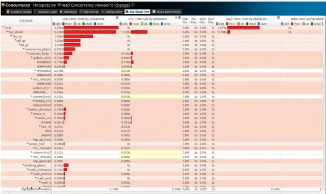
4.3 Intel VTune Amplifier . . . 32
4.4 Materials . . . 34
4.5 Datasets . . . 38
4.6 Known Issues . . . 42
x CONTENTS
5 Results 43
5.1 Initial Measurements . . . 43
5.1.1 Loading Data Files . . . 43
5.1.2 Sequential Execution Times . . . 44
5.2 Scheduling Methods Evaluation . . . 44
5.2.1 Varying Scheduling Strategies . . . 45
5.2.2 Load Balancing . . . 49
5.2.3 Varying Chunk Sizes . . . 50
5.3 Varying Data Sizes . . . 51
6 Conclusions and Future Work 61 6.1 Main Contributions . . . 61
6.2 Further Work . . . 62
6.3 Final Remark . . . 63
A Walltime Data 65 A.1 Dynamic Scheduling . . . 65
A.1.1 MAMMO . . . 65
A.1.2 BLOG . . . 68
A.1.3 PROB . . . 69
A.1.4 ODD . . . 70
A.2 Static Scheduling . . . 73
A.2.1 MAMMO . . . 73
A.2.2 BLOG . . . 74
A.2.3 PROB . . . 77
A.2.4 ODD . . . 78
A.3 Single-step Scheduling . . . 79
A.3.1 MAMMO . . . 79
A.3.2 BLOG . . . 82
A.3.3 PROB . . . 83
A.3.4 ODD . . . 84
A.4 Workpool Scheduling . . . 87
A.4.1 MAMMO . . . 87
A.4.2 BLOG . . . 87
A.4.3 PROB . . . 88
A.4.4 ODD . . . 89
B Load Balancing Data 91 B.1 Dynamic Scheduling . . . 91
B.2 Static Scheduling . . . 96
B.3 Single-step scheduling . . . 100
C Variation of Chunk Size 105 C.1 Dynamic Scheduling . . . 105
C.2 Static Scheduling . . . 108
C.3 Workpool Scheduling . . . 109
List of Figures
2.1 Example of basic Prolog program . . . 7
2.2 Example of basic Prolog queries and answers. . . 8
2.3 Pseudocode for map and reduce operations . . . 11
2.4 Graphic example of a MapReduce operation. . . 12
2.5 Example of MapReduce master-slave architecture . . . 13
3.1 Framework architecture . . . 17
3.2 Single-step scheduling method. . . 20
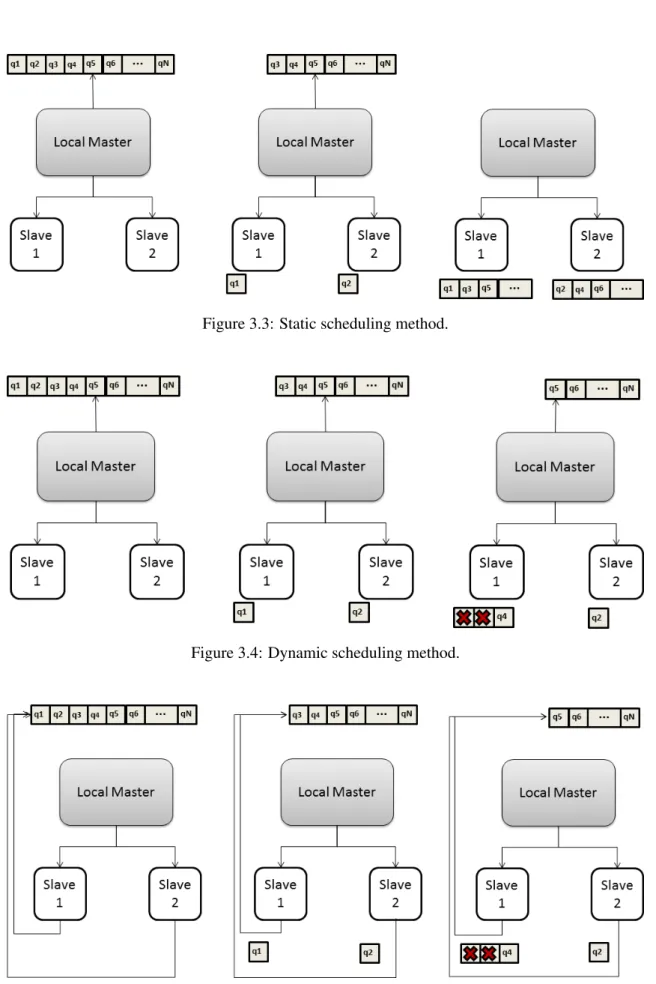
3.3 Static scheduling method. . . 21
3.4 Dynamic scheduling method. . . 21
3.5 Workpool scheduling method. . . 21
3.6 MapReduce for Prolog predicates in shared memory architectures. . . 22
3.7 MapReduce for Prolog usage example for shared memory architecture . . . 23
3.8 MapReduce for Prolog usage example for distributed memory architecture . . . . 23
4.1 Organization of the Yap system (courtesy of Ricardo Rocha, from [1]). . . 25
4.2 Organization of the Yap database (courtesy of Ricardo Rocha, from [1]). . . 26
4.3 Blocking predicate to receive a message from a queue. . . 27
4.4 Non-blocking predicate to receive a message from a queue. . . 28
4.5 Time measuring predicates kindly made available by Miguel Areias. . . 28
4.6 Example of an MPI program in Yap. . . 29
4.7 map_reduce/5implementation details. . . 30
4.8 Auxiliar predicates in work distribution. . . 31
4.9 Dynamic scheduling implementation details. . . 32
4.10 Intel VTune Amplifier Hotspot analysis. . . 33
4.11 Intel VTune Amplifier lock detection. . . 33
4.12 Machines’ storage facility, located in DCC. . . 35
4.13 Machines’ front view. . . 36
4.14 Machines’ front view - detailed. . . 36
4.15 DellTMPowerEdgeTMR905 Architecture, from [2] . . . 37
4.16 Map and reduce operations for dataset ODD. . . 38
4.17 Map and reduce operations for dataset PROB. . . 39
4.18 Map and reduce operations for dataset MAMMO. . . 40
4.19 Map and reduce operations for dataset BLOG. . . 41
5.1 Comparison of scheduling methods for ODD dataset (600,000 queries and 1,000 elements per chunk) . . . 45
5.2 Comparison of scheduling methods for PROB dataset (600,000 queries and 1,000 elements per chunk) . . . 46
xii LIST OF FIGURES
5.3 Comparison of scheduling methods for MAMMO dataset (600,000 queries and 1,000 elements per chunk) . . . 47
5.4 Comparison of scheduling methods for BLOG dataset (600,000 queries and 1,000 elements per chunk) . . . 48
5.5 Load balancing for different scheduling methods (1,200,000 queries and 1,000 elements per chunk) . . . 49
5.6 Effect of chunk size variation in dynamic scheduling (1,200,000 queries) . . . 50
5.7 Effect of chunk size variation in static scheduling (1,200,000 queries) . . . 51
5.8 Effect of variation of queries size with dynamic scheduling in ODD dataset (1,000 elements per chunk) . . . 52
5.9 Effect of variation of queries size with dynamic scheduling in PROB dataset (1,000 elements per chunk) . . . 53
5.10 Effect of variation of queries size with dynamic scheduling in MAMMO dataset (1,000 elements per chunk) . . . 54
5.11 Effect of variation of queries size with dynamic scheduling in BLOG dataset (1,000 elements per chunk) . . . 55
5.12 Effect of variation of queries size with static scheduling in ODD dataset (1,000 elements per chunk) . . . 56
5.13 Effect of variation of queries size with static scheduling in PROB dataset (1,000 elements per chunk) . . . 57
5.14 Effect of variation of queries size with static scheduling in MAMMO dataset (1,000 elements per chunk) . . . 58
5.15 Effect of variation of queries size with static scheduling in BLOG dataset (1,000 elements per chunk) . . . 59
List of Tables
4.1 Data type and background knowledge file size . . . 38
5.1 Set-up times (in seconds) for varying dataset sizes . . . 44
5.2 Sequential execution times (in milliseconds) for SMA and varying dataset sizes . 44 5.3 Sequential execution times (in milliseconds) for DMA and varying dataset sizes . 44 A.1 MAMMO DMA 300k (1000 elems/chunk) . . . 65
A.2 MAMMO SMA 300k (1000 elems/chunk) . . . 66
A.3 MAMMO DMA 600k (1000 elems/chunk) . . . 66
A.4 MAMMO SMA 600k (1000 elems/chunk) . . . 66
A.5 MAMMO DMA 1200k (1000 elems/chunk) . . . 66
A.6 MAMMO SMA 1200k (1000 elems/chunk) . . . 67
A.7 BLOG DMA 300k (1000 elems/chunk) . . . 68
A.8 BLOG SMA 300k (1000 elems/chunk) . . . 68
A.9 BLOG DMA 600k (1000 elems/chunk) . . . 68
A.10 BLOG SMA 600k (1000 elems/chunk) . . . 68
A.11 BLOG DMA 1200k (1000 elems/chunk) . . . 69
A.12 BLOG SMA 1200k (1000 elems/chunk) . . . 69
A.13 PROB DMA 300k (1000 elems/chunk) . . . 69
A.14 PROB SMA 300k (1000 elems/chunk) . . . 69
A.15 PROB DMA 600k (1000 elems/chunk) . . . 70
A.16 PROB SMA 600k (1000 elems/chunk) . . . 70
A.17 PROB DMA 1200k (1000 elems/chunk) . . . 70
A.18 PROB SMA 1200k (1000 elems/chunk) . . . 70
A.19 ODD DMA 300k (1000 elems/chunk) . . . 71
A.20 ODD SMA 300k (1000 elems/chunk) . . . 71
A.21 ODD DMA 600k (1000 elems/chunk) . . . 71
A.22 ODD SMA 600k (1000 elems/chunk) . . . 71
A.23 ODD DMA 1200k (1000 elems/chunk) . . . 72
A.24 ODD SMA 1200k (1000 elems/chunk) . . . 72
A.25 MAMMO DMA 300k (1000 elems/chunk) . . . 73
A.26 MAMMO SMA 300k (1000 elems/chunk) . . . 73
A.27 MAMMO DMA 600k (1000 elems/chunk) . . . 73
A.28 MAMMO SMA 600k (1000 elems/chunk) . . . 74
A.29 MAMMO DMA 1200k (1000 elems/chunk) . . . 74
A.30 MAMMO SMA 1200k (1000 elems/chunk) . . . 74
A.31 BLOG DMA 300k (1000 elems/chunk) . . . 74
A.32 BLOG SMA 300k (1000 elems/chunk) . . . 75
xiv LIST OF TABLES
A.33 BLOG DMA 600k (1000 elems/chunk) . . . 75
A.34 BLOG SMA 600k (1000 elems/chunk) . . . 75
A.35 BLOG DMA 1200k (1000 elems/chunk) . . . 75
A.36 BLOG SMA 1200k (1000 elems/chunk) . . . 76
A.37 PROB DMA 300k (1000 elems/chunk) . . . 77
A.38 PROB SMA 300k (1000 elems/chunk) . . . 77
A.39 PROB DMA 600k (1000 elems/chunk) . . . 77
A.40 PROB SMA 600k (1000 elems/chunk) . . . 77
A.41 PROB DMA 1200k (1000 elems/chunk) . . . 78
A.42 PROB SMA 1200k (1000 elems/chunk) . . . 78
A.43 ODD DMA 300k (1000 elems/chunk) . . . 78
A.44 ODD SMA 300k (1000 elems/chunk) . . . 78
A.45 ODD DMA 600k (1000 elems/chunk) . . . 79
A.46 ODD SMA 600k (1000 elems/chunk) . . . 79
A.47 ODD DMA 1200k (1000 elems/chunk) . . . 79
A.48 ODD SMA 1200k (1000 elems/chunk) . . . 79
A.49 MAMMO DMA 300k (1000 elems/chunk) . . . 80
A.50 MAMMO SMA 300k (1000 elems/chunk) . . . 80
A.51 MAMMO DMA 600k (1000 elems/chunk) . . . 80
A.52 MAMMO SMA 600k (1000 elems/chunk) . . . 80
A.53 MAMMO DMA 1200k (1000 elems/chunk) . . . 81
A.54 MAMMO SMA 1200k (1000 elems/chunk) . . . 81
A.55 BLOG DMA 300k (1000 elems/chunk) . . . 82
A.56 BLOG SMA 300k (1000 elems/chunk) . . . 82
A.57 BLOG SMA 600k (1000 elems/chunk) . . . 82
A.58 BLOG SMA 600k (1000 elems/chunk) . . . 82
A.59 BLOG DMA 1200k (1000 elems/chunk) . . . 83
A.60 BLOG SMA 1200k (1000 elems/chunk) . . . 83
A.61 PROB DMA 300k (1000 elems/chunk) . . . 83
A.62 PROB SMA 300k (1000 elems/chunk) . . . 83
A.63 PROB DMA 600k (1000 elems/chunk) . . . 84
A.64 PROB SMA 600k (1000 elems/chunk) . . . 84
A.65 PROB DMA 1200k (1000 elems/chunk) . . . 84
A.66 PROB SMA 1200k (1000 elems/chunk) . . . 84
A.67 ODD DMA 300k (1000 elems/chunk) . . . 85
A.68 ODD SMA 300k (1000 elems/chunk) . . . 85
A.69 ODD DMA 600k (1000 elems/chunk) . . . 85
A.70 ODD SMA 600k (1000 elems/chunk) . . . 85
A.71 ODD DMA 1200k (1000 elems/chunk) . . . 86
A.72 ODD SMA 1200k (1000 elems/chunk) . . . 86
A.73 MAMMO SMA 300k (1000 elems/chunk) . . . 87
A.74 MAMMO SMA 600k (1000 elems/chunk) . . . 87
A.75 MAMMO SMA 1200k (1000 elems/chunk) . . . 87
A.76 BLOG SMA 300k (1000 elems/chunk) . . . 88
A.77 BLOG SMA 600k (1000 elems/chunk) . . . 88
A.78 BLOG SMA 1200k (1000 elems/chunk) . . . 88
A.79 PROB SMA 300k (1000 elems/chunk) . . . 88
LIST OF TABLES xv
A.81 PROB SMA 1200k (1000 elems/chunk) . . . 89
A.82 ODD SMA 300k (1000 elems/chunk) . . . 89
A.83 ODD SMA 600k (1000 elems/chunk) . . . 89
A.84 ODD SMA 1200k (1000 elems/chunk) . . . 90
B.1 MAMMO DMA 1200k 16 slaves (1000 elems/chunk) . . . 91
B.2 PROB DMA 1200k 16 slaves (1000 elems/chunk) . . . 92
B.3 BLOG DMA 1200k 8 slaves (1000 elems/chunk) . . . 92
B.4 ODD DMA 1200k 16 slaves (1000 elems/chunk) . . . 93
B.5 MAMMO SMA 1200k 16 slaves (1000 elems/chunk) . . . 93
B.6 PROB SMA 1200k 16 slaves (1000 elems/chunk) . . . 94
B.7 BLOG SMA 1200k 16 slaves (1000 elems/chunk) . . . 94
B.8 ODD SMA 1200k 16 slaves (1000 elems/chunk) . . . 95
B.9 MAMMO DMA 1200k 16 slaves (1000 elems/chunk) . . . 96
B.10 PROB DMA 1200k 16 slaves (1000 elems/chunk) . . . 96
B.11 BLOG DMA 1200k 8 slaves (1000 elems/chunk) . . . 97
B.12 ODD DMA 1200k 16 slaves (1000 elems/chunk) . . . 97
B.13 MAMMO SMA 1200k 16 slaves (1000 elems/chunk) . . . 98
B.14 PROB SMA 1200k 16 slaves (1000 elems/chunk) . . . 98
B.15 BLOG SMA 1200k 16 slaves (1000 elems/chunk) . . . 99
B.16 ODD SMA 1200k 16 slaves (1000 elems/chunk) . . . 99
B.17 MAMMO DMA 1200k 16 slaves (1000 elems/chunk) . . . 100
B.18 PROB DMA 1200k 16 slaves (1000 elems/chunk) . . . 100
B.19 BLOG DMA 1200k 8 slaves (1000 elems/chunk) . . . 101
B.20 ODD DMA 1200k 16 slaves (1000 elems/chunk) . . . 101
B.21 MAMMO SMA 1200k 16 slaves (1000 elems/chunk) . . . 102
B.22 PROB SMA 1200k 16 slaves (1000 elems/chunk) . . . 102
B.23 BLOG SMA 1200k 16 slaves (1000 elems/chunk) . . . 103
B.24 ODD SMA 1200k 16 slaves (1000 elems/chunk) . . . 103
C.1 MAMMO DMA 1200k (16 slaves) . . . 105
C.2 MAMMO SMA 1200k (16 slaves) . . . 105
C.3 BLOG DMA 1200k (8 slaves) . . . 106
C.4 BLOG SMA 1200k (16 slaves) . . . 106
C.5 PROB DMA 1200k (16 slaves) . . . 106
C.6 PROB SMA 1200k (16 slaves) . . . 106
C.7 ODD DMA 1200k (16 slaves) . . . 106
C.8 ODD SMA 1200k (16 slaves) . . . 107
C.9 MAMMO DMA 1200k (16 slaves) . . . 108
C.10 MAMMO SMA 1200k (16 slaves) . . . 108
C.11 BLOG DMA 1200k (8 slaves) . . . 108
C.12 BLOG SMA 1200k (16 slaves) . . . 108
C.13 PROB DMA 1200k (16 slaves) . . . 109
C.14 PROB SMA 1200k (16 slaves) . . . 109
C.15 ODD DMA 1200k (16 slaves) . . . 109
C.16 ODD SMA 1200k (16 slaves) . . . 109
C.17 MAMMO SMA 1200k (16 slaves) . . . 110
C.18 BLOG SMA 1200k (16 slaves) . . . 110
xvi LIST OF TABLES
Abbreviations
API Application Programming Interface
DCC Departamento de Ciência de Computadores DMA Distributed Memory Architecture
GM Global Master
HDFS Hadoop Distributed File System ILP Inductive Logic Programming IP Internet Protocol
LM Local Master
Prolog PROgrammation en LOGique MPI Message Passing Interface SL Slave
SLD Selective Linear Definite SMA Shared Memory Architecture WAM Warren Abstract Machine Yap Yet Another Prolog
Chapter 1
Introduction
In the modern world there is a growing need for the efficient processing of immense amounts of data in a simple and incisive way. Hardware is becoming increasingly more complex and pow-erful, as well as much more affordable, due to competitive manufacturing processes and greater economies of scale. In particular, the vulgarization of multicore processors presents a clear oppor-tunity for taking advantage of these components’ architecture in order to significantly shorten task processing times using parallelism, even in a common personal laptop. As such, there is an emerg-ing demand for straightforward parallel interfaces for otherwise computationally taxemerg-ing tasks, in which users will not necessarily have an extensive programming background.
Logic Programming is strongly based on mathematical and logical concepts, making it an accessible tool for users with relatively little programming experience but a relevant scientific background, and allows for implicit parallelization by hiding implementation details from the pro-grammers. The distinct declarative style of Prolog makes it an ideal tool for analysing, processing or making inferences about data, having applications on a wide range of areas of knowledge, such as machine learning [3], natural language processing [4] or program analysis [5], among many oth-ers. The Prolog language also presents an interesting alternative to standard relational databases, having some relevant applications in this area as well [6]. Furthermore, declarative languages are typically very high level languages, meaning that the Prolog’s syntax is mostly independent of its low level implementation. This allows users to detach their algorithms from almost any concern with technical detail, since compilers already implement effective translation mechanisms.
In addition to ease-of-use, Prolog’s non-determinism allied to its declarative semantics invite the use of parallelism as a tool to improve program efficiency, without increasing the program’s complexity whatsoever. The aim of this work is then to introduce a widely known parallel pro-gramming model - MapReduce - into the Prolog language, by designing and implementing an API native to the Yap Prolog system [1]. The original MapReduce model [7] allows for handling data throughout a cluster of machines, thus processing it in parallel and under a distributed architecture. This system is composed of two user-defined operations - Map and Reduce - which conduce to an extremely flexible programming model due to their structure.
Prolog is a programming language specially suited to store and analyze data, and even to make 1
2 Introduction
inferences based on that data. This is a feature that is increasingly more requested by programmers, but the scalability of the existing data analyzing tools in Prolog has often been questioned. The aim of this MapReduce for Prolog implementation is to provide the language – and the Yap system in particular – with a flexible and easy-to-use framework for data processing in Prolog, with focus on native data types. The MapReduce programming model is an ideal choice, since it is both well-known and straightforward, presenting programmers with an attractive framework, which hides all parallelization details but whose performance is efficient.
The MapReduce construct presented in this document can not only establish a processing grid within a cluster of machines, but it can also take advantage of multicore processors in each machine, if they exist. The latter feature is found to be especially relevant now that most processors being built already incorporate at least two physical cores. Our implementation of a MapReduce construct is aimed at relatively modest computing capabilities, and small to medium dataset sizes. Under these conditions, it has proved to be agile and flexible, as well as highly efficient in terms of speeding-up process executions for both computing and logical applications.
1.1
Thesis Purpose
Due to the vulgarization and growing affordability of computers, it is now common for people to have access to more than one machine. In the last decade these machines were often equipped with multicore processors, which have gained increasing significance as a standardized and inex-pensive option. Both these facts combined provide ample possibilities for software designers to take advantage of this emerging type of architecture composed of several machines with multicore processors but relatively modest capabilities.
This thesis’ contribution lies in the fact that the MapReduce Construct for Prolog is applicable to both multicore processors and clusters of machines, thus attaining high efficiency and much shorter processing times in running tasks, while still using a straightforward declarative semantic which implements the MapReduce model. This model is composed of two very basic operations which are widely suitable for the processing of data concerning various applications [8]. It could be argued that the lack of complexity of this model renders it trivial research-wise, nevertheless we find that its simplicity is one of the key features which makes the paradigm so widely accepted and used.
Logic Programming could be considered an unusual choice to implement a MapReduce model since its focus is not on implementation details such as basic parallel constructs (threads or pro-cesses); however, it presents an unique suitability to store facts in a background knowledge form and draw conclusions from them, whilst it can still efficiently process most other forms of data. Some criticisms have been made to logic programming languages regarding the reduced autonomy of the programmer in terms of system definition and parallel optimization. This work addresses that issue by implementing several possible levels of customization, from basic usage of the con-struct to the definition of a grid of machines with their respective IP addresses and multicore ar-chitectures. We hope this will effectively accommodate needs from users with strikingly different
1.2 Thesis Outline 3
goals and backgrounds.
1.2
Thesis Outline
This document is structured in 6 chapters, reflecting the different stages of the work. A brief description for each one is provided below.
Chapter 1: Introduction. The current chapter.
Chapter 2: Background and Related Work. Presents relevant information on both logic pro-gramming and MapReduce systems. In the first section, Prolog language basics such as first order logic and Horn clauses are briefly described, followed by some examples of Prolog syntax and semantics and an explanation regarding the various types of parallelism that can be exploited in this language. This section also includes an overview of the Yap Prolog sys-tem and of declarative programming in general. The latter section defines the MapReduce model and addresses several implementations described in the literature. It then details the most relevant works to this thesis, providing an in-depth analysis of their features.
Chapter 3: MapReduce in Prolog. The design of the system is detailed in this chapter, both for clusters and for multicore architectures. The interface is also presented, as well as some relevant examples of usage.
Chapter 4: Methodology. This chapter includes a thorough description of the datasets used to validate the implementation. There is also an account of the machines used, as well as the evaluation parameters for the results presented in the following chapter. In addition, the Yap Prolog file system is introduced and a number of modifications and difficulties encountered are detailed here. Some of the most relevant Yap Prolog libraries are briefly mentioned as well.
Chapter 5: Results. This section contains firstly a quantitative account of the results from the experiments with the system. Here are included the speedup plots and other measurements considered pertinent to the systems’ assessment. The second part of this chapter contains a qualitative description and discussion of the results, in order to provide some insight on relevant points.
Chapter 6: Conclusions and Future Work. The work is summed up and some suggestions for the future are detailed.
Chapter 2
Background and Related Work
This chapter contains a summary of relevant state-of-the-art for both Logic Programming and the MapReduce model. The Prolog language is introduced in some detail, and examples of usage are provided. An explanation on how different forms of parallelism can be applied, with reference to those examples, serves as preamble for the description of the MapReduce model. A number of MapReduce implementations are presented and finally, an application of MapReduce to Logic Programming is described in some detail, since it is a pertinent start point for this work.
2.1
Logic Programming
Since the mid-1900’s until the present time numerous programming languages have been devel-oped. As such, a need arose to identify common features amongst the programming languages so as to classify them accordingly. Therefore, four main paradigms have emerged from this pro-cess, matching every programming language to one of these categories: imperative programming, functional programming, logic programming or object-oriented programming. Imperative pro-gramming’s semantic is composed of strict translations from machine language to a set of user commands, whilst functional programming is concerned with features such as recursion or pat-tern matching. Object oriented languages are the most recent paradigm and are versatile and very complete in terms of functionalities. Declarative languages are also a relatively recent paradigm – stemming from functional programming – and they aim at creating a dettachment between a pro-gram’s goal and its execution details by enhancing the functional characteristics of the language in preference to its technicalities. This allows the programmer to focus on the way in which the program should be executed rather than how the actual computation is performed; the program-ming task then becomes both easier and more efficient, as stated by J. W. Lloyd in [9]. Logic programming languages are a subset of declarative languages, meaning that the programmer is only required to specify what a program should do, and the language is responsible for executing the specification in a fairly efficient way. It is evident that this paradigm of programming allows for a detachment between the logic goals of the program and its execution goals, which can be ex-plored towards greater efficiency. There are various languages in the logic programming category
6 Background and Related Work
(such as the Datalog [10] or Godel [11] languages), but only the Prolog family will be discussed here since the remaining languages are out of the scope of this work. Prolog first appeared in 1972 [12], in result of extensive research on an experiment whose aim was to develop a strategy for computers to interpret natural language. Since then, it has evolved and branched out into a number of distributions such as SWI-Prolog [13], SICStus Prolog [14] or Yap [1].
2.1.1 The Prolog Language
In 1969, Cordell Green developed an automatic theorem proving procedure [15] applicable to first-order logic systems, from where stem the numerous declarative programming languages in existence today. Prolog’s syntax, in particular, is composed of clauses that can be expressed as a conjunction of literals, also known as Horn clauses. This type of logical construction is a subgroup of first-order logic, and as such it is not only resoluble and complete given a set of axioms but it is also closed: the resolvent of two Horn clauses is also a Horn clause. This fact makes it possible and convenient to recursively solve these clauses using resolution methods based on SLD [15].
In 1983, David Warren introduced a memory architecture and an instruction set, later named the Warren Abstract Machine [16], meant to efficiently translate Prolog instructions to lower level code, then to be resolved. The WAM still presently sets a relevant standard amongst Prolog com-pilers [17]. It is important to note that whilst the order of the terms in a clause is mathematically indifferent, it can be computationally taxing. More recent additions have been made to WAM and other abstract machines in order to decrease the side-effects caused by parallel term computation, deriving from the use of Or and And parallelism, to be described later.
Prolog is then a language composed of rules and terms, and their mutual interaction. It has been argued that the logic programming paradigm should have been named the relational program-ming paradigm [9] since that terminology better describes the nature of the language. A term is the basic Prolog language entity, and it can be an atom (starts with lower-case letters or is enclosed in single quotation marks), a number (float, integer), or a compound term (also named a functor). An example of the latter would be a Prolog list such as [L1, L2, ..., LN]. A term can also be a free variable (its name starts with an uppercase letter or an underscore) which is type-less until it is unified, meaning that a value is then assigned to the variable. Since Prolog has no destructive assignment of variables, unification for each variable can occur only once. However, backtracking allows for unbinding already unified variables, since Prolog stores choicepoints and can restore a previous program state so as to explore all possible solutions.
A rule in Prolog is necessarily a Horn clause, composed by a head and a body, and follows the structure presented in Equation2.1.
head: −body_clause1, body_clause2, ...body_clauseN. (2.1)
2.1 Logic Programming 7
true, the body must also be true. A rule can have no body – the equivalent to2.2.
head: −true. (2.2)
In these cases the rule is named a fact and represents a logical tautology in the program’s scope. The set of rules and facts of a Prolog program is called its clauses. The rule names in a program are also called predicates, and a predicate can have several clauses with different arity (number of predicate arguments). The body of a rule is composed of a sequence of goals, interacting with one another through connectives, or operators; in this case ,/2 corresponds to the AND connective. Each goal represents a call to a predicate, which is then determined to be true or false. It is thus evident that the execution of a Prolog program requires both a goal selection rule to determine which goal is to be called next, and a search rule to choose which alternative of a goal to explore, if several exist. Prolog’s resolution employs left-to-right goal selection and an depth-first search strategy, and each resolution step taken is called reduction or logical inference. Since Prolog is a programming language and thus not purely logical, it requires meta and extra-logical predicates such as input/output operations, arithmetic operations or the cut operator. The latter must be used under some circumstances for program correction, and it can also be helpful in expediting execution by pruning the search tree and thus set aside unexploited alternatives. This operator is an example of a non-logic predicate since it is sensitive to the order in which the goals are exploited. Figure2.1gives an example of a basic Prolog program illustrating most of these concepts. In cat ( tom ).
mouse ( jerry ). cheese ( roquefort ). cheese ( emmental ).
eats (X ,Y):- cat (X) , mouse (Y). eats (X ,Y):- mouse (X) , cheese (Y).
Figure 2.1: Example of basic Prolog program
this program there are four assertions, or facts: tom is a cat, jerry is a mouse and roquefort and emmental are both cheese. There is also a rule, or predicate, composed of a head eats(X,Y) and a body containing the definition of eating. This rule expresses the fact that either cats eat mice (first clause of eats/2) or mice eat cheese (second clause of eats/2). Figure2.2contains some queries one could now pose regarding the program above (see Figure2.1).
When analysing Figures 2.1 and 2.2 it becomes evident that the two parts - or clauses - of the predicate eats(X,Y) are independent from each other in the sense that they do not have side effects on one another. The fact that tom is a cat is detached from the fact that emmental is a type of cheese, and so it follows that these calculations could be made simultaneously and that would not alter the final answer of the query. This simple example serves to demonstrate the fitness of Prolog languages to the application of implicit parallel execution, which will be discussed in more
8 Background and Related Work
?- eats ( Anything , tom ). no
?- eats (tom , Anything ). Anything = jerry ? ;
no
?- eats ( jerry , Anything ). Anything = roquefort ? ;
Anything = emmental .
Figure 2.2: Example of basic Prolog queries and answers.
detail in the following section.
2.1.2 Parallelism in Prolog
Parallelism in the Computer Science domain means to split a program in concurrent parts and ex-ecute them simultaneously. This if often done with multi-threading, using only one machine, but it can also support many machines running the same program at once. Also, parallelism can be divided in two categories, depending of how aware the user is of the parallelization mechanism. Implicit parallelism takes place when the programmer writes the code as if it were going to be executed sequentially and the system is responsible for executing the code concurrently, for faster and more efficient execution when compared to the sequential case. Explicit parallelism typically obtains even better results in terms of efficiency, since the user can tune the system for optimum performance. This, however, requires systems to provide a framework in which the user can decide how he/she wants to run the program in a parallel way. These two forms of parallelism have radi-cally different applications and implementations, and the focus of this document is on an explicit parallel model; however, we explore it implicitly by default, hiding the parallelization details from the user. Different levels of explicit parallelism can easily be incorporated in the MapReduce for Prolog construct presented in this document because it provides different levels of customization, rendering it possible for more experienced users to explicitly call parallel predicates in the system. According to [18] there are three ways in which implicit parallelism can be explored in Prolog lan-guages: And-parallelism, Or-parallelism and unification parallelism. A brief description of each follows, with reference to Figs2.1and2.2.
And-parallelism can be used when there is more than one subgoal in a resolvent, meaning that the parallel executions either compete or cooperate to find a solution. This type of parallelism can be dependent or independent, depending on whether there are variables common to the branches which have not been unified prior to the query. Independent and-parallelism could be applied given the following query: ?-eats(Something,Anything)., since it can be broken down as two clauses: cat(Something),mouse(Anything)., which could both
2.1 Logic Programming 9
be executed simultaneously. An example of dependent and-parallelism would be ?-eats( Something,Something)., using the same break-down structure.
Or-parallelism can be applied when more than one rule head unifies with a query. Thus, the tion space is searched concurrently, and in effect each search can lead to different valid solu-tions. This form of parallelism applies when a query such as eats(Something,Anything ).is called, since there are two different clauses corresponding to the eats/2 predicate. Unification parallelism can exist when a term with arity greater than one needs to be unified. In
such a case, the unification of its arguments can be done in parallel: eats(jerry,cheddar )=eats(Mouse,Cheese).. In this case, the variables Mouse and Cheese can be bound to jerryand emmental values concurrently.
Most Prolog systems currenlty available do not support parallelism [18]. The Yap and the SICStus Prolog are two examples of systems that support implicit or-parallelism. Also, some systems such as Yap or SWI Prolog maintain explicit parallel constructs (for instance, thread support).
2.1.3 The Yap System
Yet Another Prolog system [1] first appeared in 1984 in University of Porto and presented a WAM based design with some improvements, namely a very fast emulator written in assembly [1]. How-ever, in the mid 90’s some portability issues regarding the system emulator assembly code raised, forcing the Yap developers to revert to a C-based emulator, which at first proved to be much slower, but whose performance has increased greatly over the past years [19]. Also, at this point, some additions were made to the Yap system so as to support parallelism [20] and tabling mechanisms [21]. Because Yap is meant to provide support not only for small applications, but also for ap-plications which require the manipulation of large and complex databases, in the past few years three very important additions have been made to the system. From [1] a short summary of these features is presented below.
The Just-In-Time Indexer (JITI) allows for indexation of both multiple arguments, compound terms and multiple modes of usage. Even though JITI can have a cost in terms of memory usage, it is generally thought that the advantages in runtime outweigh it [22].
The Sequential Tabling Engine provides runtime support for sequential and dynamic mixed-strategy tabling. This mechanism has proved yield good result when compared to other Prolog systems in the literature [23], [24].
The Or-Parallel Tabling Engine uses incremental stack copying to increase runtime speeds, and it has been shown in [24] that this methodology is successful for systems with medium parallelism.
10 Background and Related Work
Yap is one of the fastest Prolog systems in existence, being highly portable due to its C source code and very complete, integrating several modules of I/O operations, threads and databases. The work described in this document is implemented on top of the Yap system.
2.2
The MapReduce Framework
MapReduce is a programming model developed by Google in the early 2000’s [7] aimed at pro-cessing large amounts of data. As the name suggests, it is composed of two elementary operations: mapand reduce, which are based on primitives originally introduced in functional programming languages such as Lisp. The map operation applies a transformation to a set of key/value pairs, resulting in another set of the same size consisting of pairs with the same key but a mapped value. The reduce operation groups all the mapped pairs with the same key and aggregates their values, usually into one - or no - result. The pseudocode in Figure2.3illustrates the functions described before. The aux_aggregator operation is independent of both the data being processed and the map and reduce operations, rendering it autonomous from the remaining program; this operation allows the user to run different kinds of data on the same MapReduce call and group then using a key. This feature is specific to Google’s MapReduce implementation and it is not included in the MapReduce for Prolog construct because it was found to be unnecessary. The size of the datasets our construct is aimed at does not justify burdening the framework with another mandatory oper-ation and since MapReduce for Prolog can be used iteratively, the user can simply make one call for each data type in a loop.
Figure2.4depicts a very simple MapReduce operation. In that case, the inputs are squares, triangles and circles, either black or white. The colour of the shapes represents their key and the shape itself is the value. The mapping process transforms each shape into the first letter of its name, thus mapping a square to an S, a triangle to a T, and so on. The mapped values are then sorted by colour, corresponding to the aux_aggregator operation, and finally the reduce function is called. This function consists of counting how many T’s there are. Thus, the result of the operation per key is found to be 2 white T’s and 1 black T.
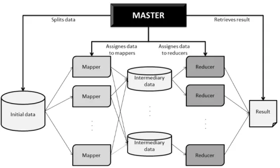
The MapReduce model was primarily developed to be applied onto a large set of machines linked together - also known as a cluster - with the purpose of drastically reducing data processing times by taking advantage of the parallel architecture of this system. Most MapReduce frameworks described in the literature [7,25,26,27,28,29], if not all, use a master-slave architecture, similar to the one presented in Figure2.5. Figure2.5 depicts the flow of data in a generic MapReduce application. The data flows from left to right and is controlled by the Master. The initial data is assigned to one of the Mappers, and through computation is transformed into Intermediary data. The Master then assignes Reducers with some of the Intermediary data and after the reduce operations take place, the result is determined. Given the sometimes huge size of the clusters in which MapReduce frameworks are applied (consider the architecture in [7]), they must be highly fault-tolerant and robust. Amongst other precautions mentioned in the literature, the master node
2.2 The MapReduce Framework 11
map_operation (key , value ) -> (key , mapped_value ) { mapped_value = perform_map_operation ( value ); }
reduce_operation (key , set_of ( mapped_value )) -> (key , reduced_value ) {
reduced_value = perform_reduce_operation ( set_of ( mapped_value ) );
}
aux_aggregator ( set_of (key , mapped_value )) -> set_of (key , set_of ( mapped_value )) {
for each key compute
set_of ( mapped_value ) = aggregate_by_key (key , set_of (key , mapped_value ));
}
Figure 2.3: Pseudocode for map and reduce operations
is usually responsible for pinging the slave nodes, as well as backing up the processed data and rescheduling work in case of slave failure.
So far, the features of the MapReduce paradigm have been superficially described, but nothing has been said regarding its capability to meet real-world data processing requirements. The rele-vance of this model lies in the fact that the map and reduce operations are suitable for expressing a number of classic processing algorithms under a summation form [8]. This form allows for a direct conversion to map and reduce operations, and it has been shown by [8] that algorithms such as lo-cally weighted linear regression, expectation maximization and neural networks, amongst others, can be applied successfully to a MapReduce framework.
Whilst these algorithms can be useful, the MapReduce model is by no means limited to them, as many possible map and reduce operations can be defined for this framework. One needs only to ensure that the operations have no collateral effects on data other than that being used in the operation. Furthermore, it is necessary to guarantee that the operations on the data are associa-tive and commutaassocia-tive, so that they can be executed in parallel and thus benefit from the inherent speeding up of the process. This speed-up is a pertinent indicator to evaluate the performance of a MapReduce framework running in parallel, and in this document the following metrics for system speed-up will be adopted:
Su=
Ts
Tu
(2.3) where
Suis the system speed-up for u processing units. If Suis greater than 1, the system is faster than
12 Background and Related Work
Figure 2.4: Graphic example of a MapReduce operation.
Tsis the time the system takes to run a sequential execution of the problem.
Tuis the time the system takes to run with u processing units.
The number of processing units in a system is considered to be the number of workers running simultaneously during a given call. The ideal and maximum number of processing units for a system can then be calculated as:
U= M
∑
m=1 Pm∑
p=1 Cp (2.4) whereUis the total number of processing units in the system. Mis the number of Machines in the system.
Pmis the number of Processors in machine m.
Cpis the number of Cores in processor p.
2.2.1 MapReduce Implementations
There are presently several MapReduce implementations described in the literature [7,25,26,27,
2.2 The MapReduce Framework 13
Figure 2.5: Example of MapReduce master-slave architecture
1. The HDFS or Hadoop Distributed File System [31] is a fault-tolerant distributed file sys-tem, which is designed to run on low-cost hardware. Its purpose is to meet the requirements of applications which need to manipulate large datasets and it was designed with a batch processing methodology in mind, as opposed to iterative data processing. This system uses data replication for higher reliability but also with the purpose of improving network traf-fic and data accessibility. In [27] Hadoop is compared to other approaches of large-scale data analysis, and whilst its setup time is negligible compared to others, the overall task processing time was found to be 3.2 times slower than the second slower approach tested (an SQL Database Management System) [27]. This highlights that there is still much work to be done if the MapReduce framework is to become a dominant approach in large-scale data-analysis.
2. Twister [29] presents an architecture different from other MapReduce frameworks since it provides efficient support for iterative MapReduce calls. Unlike most systems in the literature, it uses a publish/subscribe messaging protocol and attempts to reduce the amount of communication data to a minimum by increasing the granularity of the map operation. However, it does not feature any form of load balancing, nor is it highly fault tolerant. The only safeguards Twister implements are to back data up at the end of each iteration and to re-send work to slave nodes in case of failure. This approach presents slightly faster results than Hadoop in the situations described in [29].
14 Background and Related Work
3. SAGA [26] is a high level API which executes operations on distributed systems, support-ing various architectures like clusters, clouds or grids. Unlike the two previous frameworks, SAGA is implemented natively in C++, as opposed to Java, and the MapReduce model was recently introduced into it. This approach is slower than most others due to its portability; the fact that it is not optimized for one distributed system only has a cost in terms of effi-ciency. Still, it provides a simple interface for programmers to use the MapReduce model in distributed systems with less conventional architectures.
2.2.2 MapReduce Applied to Prolog
One might wonder about the relevance of creating a MapReduce framework for Prolog, since there are already several portable and flexible implementations for other programming languages in the literature, as described in the previous sections. However, Prolog provides support for features which would be difficult to implement in functional, imperative or object-oriented languages, such as natural language analysis, machine learning and, of course, inductive logic programming. ILP is the preferred Prolog application in this work because it requires intensive and iterative processing of large amounts of data so as to infere rules applicable to it. As such, a MapReduce construct would be a valuable tool to make this process simpler and more efficient. An example of such an application is then briefly described below.
In [32], Ashwin Srinivasan et al. introduce an approach combining Hadoop’s MapReduce framework [33] and the inductive logic programming system Aleph [34]. Their aim was to inves-tigate whether the ILP engine could be applicable to very large datasets, seen as the amount of data available for processing has become so large as not to fit into one machine’s memory. MapRe-duce was the selected framework for this task, due to its abstraction level and the fact that several machine learning algorithms can successfully be implemented on this model [8]. The approach used in this work consisted of two distinct engines, one for running ILP and the other for running the actual MapReduce using the Hadoop framework [31]. Two different sets of map and reduce functions were developed for this system, with different aims. The first of these sets was meant to distribute the background knowledge across the MapReduce cluster, so as to ensure that the second set of functions - which actually perform the relevant calculations for the given examples - had all the necessary clauses to be able to use a greedy algorithm. The Map Reduce and ILP engines communicate and the latter transforms examples not yet covered in MapReduce queries. When the last reduce operation is finished, the minimum cost clause determined is then returned to the ILP engine.
The authors have used both synthetic and real-world datasets, with sizes ranging from tens of thousands up to millions, and their results demonstrated that the MapReduce framework can be efficiently applied in this context. Still, the size of the dataset must be significant (greater than 500,000) in order to obtain some speed-up using this methodology. Also, the speed-ups are not nearly linear until datasets of size 5 million, and for datasets smaller than 500,000 the data processing time actually slows down when compared to sequential time due to the cost of data communication and disk access in the cluster, amongst other factors.
2.2 The MapReduce Framework 15
To the best of our knowledge, there is no MapReduce framework native to Prolog, and so the aim of this document is to describe a fast and versatile implementation of this framework in Yap. The motivation for this lies in the need for a tool for transparent distributed computing in Prolog, whose results present speed-ups even for small datasets, and whose interface would be available as predicates in a Yap library. We believe this would contribute towards more and simpler data processing support in Yap, and find it particularly relevant at an age when multi-core processors are increasingly common and inexpensive.
Chapter 3
MapReduce in Prolog
In this chapter we describe our high-level MapReduce parallel construct for Prolog and present the most relevant implementation details.
3.1
Architecture
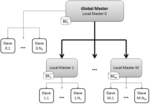
The model’s architecture is loosely based on the architecture described in [7] in the sense that it supports clusters of machines, but it innovates by taking advantage of the parallelism within each machine. Figure3.1shows how our framework can apply to a generic distributed architecture.
Figure 3.1: Framework architecture 17
18 MapReduce in Prolog
There are three hierarchical levels in this architecture: the Global Master (GM), the Local Masters(LMs) and the Slaves (SLs). The GM controls the flow of communications and first-level scheduling, dispatching data to the LMs. There are as many LMs as machines in the cluster and each LM is responsible for local data scheduling and dispatching among the SLs running on that machine. The SLs execute both map and reduce predicates on their data and return the reduced value to the respective LM. Each LM then performs a reduce operation on all its SLs’ reduced values, and similarly the GM executes the last reduce operation of the call. This architecture applies to distributed memory systems composed of multi-core machines.
For shared memory architectures (SMA), our MapReduce for Prolog uses multi-threading while for distributed memory architectures (DMA), it uses MPI [35]. In the SMA implementation, the first thread – LM0 – starts as many threads as the number of machine cores. Each thread runs a slave interface, which waits for thread messages from LM0 and carries out the work. In the DMA implementation, processes are started for each machine core or for each distributed computer node. The SLs can be thought of as resources that LMs manage according to different scheduling methods; the SLs do not keep track of how many operations they have executed, and they do not self terminate. Instead, LMs are responsible for their creation, task assignment and termination.
The system requires a set-up time, in which each LM loads any files that may have been requested by the user, so as to have the necessary information to carry out queries. This infor-mation is named background knowledge; in the case of different LMs, each one can have its own background knowledge. The set-up time is only spent once for each LM and each background knowledge file requested, for the SMA implementation. For the DMA implementation, files need to be read by all LMs. Since the data files are only loaded on LMs during the initialization of the program, this model allows for no communication overheads during runtime. Note that the user is responsible for having a copy of the program source code in each machine, as well as the map and reduce predicates and any other data required to complete the queries.
The MapReduce predicates are user-defined but follow a specific pre-defined signature. The map predicate has two arguments, the first being an element from the list of values to be mapped and the second the mapped result. The reduce predicate also has two arguments, the first being a list of Prolog terms to be reduced and the second the reduced result.
Each MapReduce call receives as arguments the names of predicates to be used to map and re-duce data. As such, the user can specify several different predicates and use them indiscriminately in different MapReduce calls without having to re-initialize the system. The MapReduce predicate also requires a data array as input. This array can be created by the user, or it can be loaded from a file automatically. Our framework includes predicates capable of creating an array of data from a given file. The positions in the array contain the respective line of the file, in the form of a generic Prolog term. We consider this to be a flexible approach, since the user can use data from any other source he/she requires, as long as he/she makes it available to the system under this structure.
3.2 File System 19
3.2
File System
One of the main goals of this implementation is to provide a flexible system, which supports both heavy computations across several machines and lighter iterative runs of MapReduce possibly executing on one machine alone. We have designed a transparent architecture divided in three functional modules as follows:
Initializer Creates a communication grid encompassing the LMs and the SLs, and loads the data for each LM.
MapReduce This module is composed of the master and the slave files. Only one of these files is used at any given time, according to the entity’s hierarchical level. The slave version ex-ecutes the map and reduce predicates, while the master version performs reduce operations and implements communication protocols.
Terminator Terminates the communication grid created by the Initializer and frees the allocated memory.
Additionally, user-defined files are required in order to specify the several map and reduce predicates to be used. The fact that this information is specified as Prolog predicates allows the user to easily reconfigure them – including system architecture and map and reduce predicates; it is also possible to run distinct MapReduce calls simultaneously.
3.3
Scheduling Methods
Most parallel and distributed MapReduce systems are not very concerned with the efficiency of scheduling strategies, rather with their redundancy and fault-tolerance strategies. Conversely, and since MapReduce for Prolog is an implementation for more modest computing capabilities, we concern ourselves with the speedup that this construct achieves, when compared to executing the MapReduce call sequentially. It is then crucial to have a scheduling method which allows for good performance in parallel, and bearing this in mind we developed four scheduling methods: (i) single-step scheduling; (ii) static scheduling; (iii) dynamic scheduling and (iv) workpool schedul-ing.
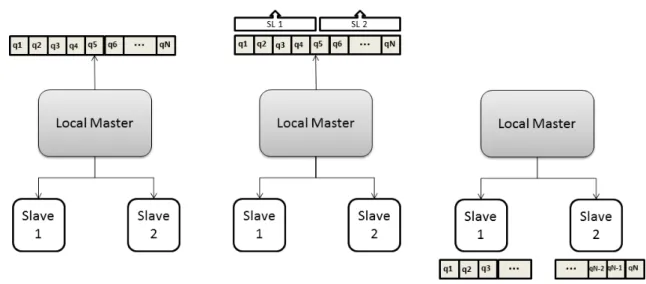
Figures 3.3, 3.4, 3.5 and 3.2 depict the interaction between LMs and SLs on each type of scheduling. This interaction can obviously extrapolate to GMs and LMs, respectively. All figures depict three stages of the scheduling algorithm, temporally from left to right, and the explanatory text is presented below.
Single-step scheduling is used as a base case. It takes the total number of items and distributes them evenly across slaves in just one step. One block of items goes to one slave, another to the second slave and so on, ensuring every SL is assigned the same number of queries, approximately. In stage two of Figure3.2, the method of dividing data is depicted, and in stage three the division is completed.
20 MapReduce in Prolog
Figure 3.2: Single-step scheduling method.
Static scheduling consists of dividing the M data items in chunks of N elements and distributing them in a round-robin fashion by all the slaves. It differs from the single-step scheduling because the queries are distributed in several small chunks, in turns. Figure3.3shows that it first attributes a chunk to each slave and from then all the data is distributed alternately by the slaves.
Dynamic scheduling is more adaptive than the previous method, but also more demanding on the LM in terms of computation time. At first, it also attributes a chunk of data to each slave, in order, but then the LM waits for a reply from one of the SLs, informing that it is free. This algorithm behaves differently from static scheduling because, as shown on stage three of Figure3.4, the LM waits for a reply from one of the SLs. The LM then attributes further work to the free SL and waits again. Ultimately, and if the data granularity is low, the dynamic scheduling converges towards static scheduling, since all SLs take the same time to complete the same number of queries.
Workpool scheduling is similar to the dynamic one, but implements a pool of work that is con-sumed on demand of idle slaves. As depicted in Figure3.5, the SLs have access to a pool of work that is filled by the LM with chunks of data to be processed. The SLs remove one chunk of work when they are finished with their current one, until the pool is empty. The LM is not responsible for distributing the work between SLs, and this can be computation-ally less taxing on the LM entity. However, the access to the workpool is heavily competed for, and more so with a growing number of SLs.
Results and other considerations on the various scheduling methods are presented in further detail in Chapters4and5, as well as some relevant future work, mentioned in Chapter6.
3.3 Scheduling Methods 21
Figure 3.3: Static scheduling method.
Figure 3.4: Dynamic scheduling method.
22 MapReduce in Prolog
3.4
User Interface
The MapReduce for Prolog user interface is composed of six predicates, as illustrated in Fig-ure3.6.
init_communicator (- Comm ).
init_communicator (- Comm ,+ NoCores ). end_communicator (+ Comm ).
data_from_file (+ Filename ,- DataArray ).
map_reduce (+ Comm ,+ MapPred ,+ ReducePred ,+ DataArray ,- Result ). map_reduce (+ Comm ,+ MapPred ,+ ReducePred ,+ DataArray ,- Result ,+
Scheduling ).
map_reduce (+ Comm ,+ MapPred ,+ ReducePred ,+ DataArray ,- Result ,+ Scheduling ,+ NoElements ).
map (+ Value ,- MappedValue ).
reduce (+ ListOfValues ,- ReducedValue ).
Figure 3.6: MapReduce for Prolog predicates in shared memory architectures.
The init_communicator/1 and init_communicator/2 predicates initialize the system: if no NoCores argument is provided, the MapReduce for Prolog determines the number of cores in the machine and starts the corresponding number of slaves. The predicate then returns the slave’s information in the Comm argument. The end_communicator/1 predicate should be used to terminate the communication grid and free memory.
The data_from_file/2 predicate can be used to consult a file and load its lines, as Prolog terms, into an array. The use of this predicate is optional, since the user may build an array from other sources and pass it as argument to the map_reduce() call. This predicate supports three levels of customization. The most basic form – map_reduce/5 – uses the standard scheduling options. The map_reduce/6 and map_reduce/7 allow the user to select a scheduling method and the number of elements per chunk for that method, if applicable. These predicates can be called iteratively and with different map and reduce operations, and they return only the final result.
Finally, the map/2 and reduce/2 are not part of the interface per se, but they are included in the description for completeness and also because even though they are user-defined, their signature must match the one in Figure3.6. These predicates define the specific map and reduce operations and their names are passed as arguments to the map_reduce/5 predicate. This allows for great flexibility, since the user can define several predicates prior to execution, as well as, for instance, specify different behaviours according to the machine the predicates are running in.
Due to the MPI communication protocol usage, the interface differs between shared memory and distributed memory architectures. The predicates for the distributed memory version do not contain the Comm argument, since the program is run as an MPI executable, meaning that the
3.4 User Interface 23
communication grid must be configured in the MPI protocol, outside the MapReduce for Prolog interface. For distributed memory systems, it is assumed that the grid has been configured and is running, and that a copy of the relevant files has been placed in every machine in the cluster. It is also not possible to change the scheduling method to workpool, since the SLs behaviour is radically different from the one exhibited in the other three scheduling methods. Other than that, the interface is very similar in both cases, and the configuration options are common to both cases. Note that the user can abstract from the details of the parallel implementation and machine architecture as we provide interfaces with different levels of transparency.
3.4.1 Usage Examples
Two usage examples are now presented in Figures3.7and 3.8. map (V ,1) :- call (V) ,!.
map (_ ,0) .
reduce ([] ,0) : -!.
reduce ([ H|T], RV ):- reduce (T , Aux ) ,RV is Aux +H. example ( Result
):-init_communicator (8 , Comm ) ,
data_from_file ( ’ queries . pl ’, MyArray ) ,
map_reduce ( Comm ,map , reduce , MyArray , Result1 ) , do_something ( Result1 , MyArray , MyNewArray ) ,
map_reduce ( Comm ,map , reduce , MyNewArray , Result2 ) , do_something ( Result1 , Result2 , Result ) ,
end_communicator ( Comm ).
Figure 3.7: MapReduce for Prolog usage example for shared memory architecture
map (V , MV ):- MV is V mod 2. reduce ([] ,0) : -!.
reduce ([ H|T], RV ):- reduce (T , Aux ) ,RV is Aux +H. example ( Result
):-data_from_file ( ’ queries . pl ’, MyArray ) ,
map_reduce ( Comm , map , reduce , MyArray , Result ) , do_something ( Result ) ,
end_communicator .
Figure 3.8: MapReduce for Prolog usage example for distributed memory architecture The map/2 predicate introduced in Figure 3.7 verifies whether a given call is true and the reduce/2predicate applied in this example sums all the numbers in a list, which calculates how
24 MapReduce in Prolog
many terms are true for map/2. This example is intended to be illustrative of a map operation native to Prolog, but there are many other possible applications for the simple but powerful frame-work we provide, such as run map_reduce/5 calls in a loop, or define map and reduce operations so as to apply the Naïve Bayes algorithm on a dataset, as described in [8], amongst other.
In Figure3.8, the map/2 predicate is an example of a generic computation, and the purpose of that MapReduce call is to determine the number of odd numbers in the queries.pl file. This illustrates the high adaptability of MapReduce for Prolog, and its ease-of-use.
Chapter 4
Methodology
This chapter contains a thorough description of the software used to complete this work, such as the Yap System, the Intel VTune Amplifier tool and openMPI. Also, modifications to the Yap system source code and some known issues are also mentioned. Finally, the datasets used in the experiments and the respective map and reduce operations are presented.
4.1
The Yap System in Detail
Even though the MapReduce for Prolog construct was implemented on the Yap system (version 6.3), some research about its internal structure was made. This was necessary in order to per-form some fine tuning required to improve the efficiency of MapReduce for Prolog; its initial results were not satisfactory. As such, slight modifications to the system have been made, and are described in further detail in Section4.3. The Yap system is then depicted in Figure4.1
Engine OPTYAP YAPOR YAPTAB YAAM Emulator Compiler Assembler JITI Clause Compiler Internal Database Libraries Prolog-Core Libraries SWI Emulation Top-Level C-Core Libraries C-Foreign Interface Threads Library User C File
YAP Prolog
User Prolog FileFigure 4.1: Organization of the Yap system (courtesy of Ricardo Rocha, from [1]).
In this system, there are four main data structures: 25

![Figure 4.1: Organization of the Yap system (courtesy of Ricardo Rocha, from [1]).](https://thumb-eu.123doks.com/thumbv2/123dok_br/18708629.917294/45.892.159.785.807.1046/figure-organization-yap-courtesy-ricardo-rocha.webp)
![Figure 4.2: Organization of the Yap database (courtesy of Ricardo Rocha, from [1]).](https://thumb-eu.123doks.com/thumbv2/123dok_br/18708629.917294/46.892.104.745.436.873/figure-organization-yap-database-courtesy-ricardo-rocha.webp)