Absorption and Emission in the Non-Poisson Case:
The Theoretical Challenge Posed by Renewal Aging
Gerardo Aquino,
Institute for Theoretical Physics, University of Amsterdam Valckenierstraat 65, 1018 XE Amsterdam, The Netherlands
Luigi Palatella,
Istituto dei Sistemi Complessi del CNR, Dipartimento di Fisica dell’Universit `a di Roma “La Sapienza”, P.le Aldo Moro 2, 00185 Roma, Italy
and Paolo Grigolini
Center for Nonlinear Science, University of North Texas, P.O. Box 311427, Denton, Texas 76203-1427 Istituto dei Processi Chimico Fisici del CNR Area della Ricerca di Pisa, Via G. Moruzzi 1,56124 Pisa, Italy
Dipartimento di Fisica dell’Universit`a di Pisa and INFM, via Buonarroti 2, 56126 Pisa, Italy
Received on 6 January, 2005
This short paper aims at clarifying the physical meaning of a previous pubblication [G. Aquino, P. Grigolini, L. Palatella, Phys. Rev. Lett. 93050601 (2004)], using later, although very recent, results. This has to do with the challenges posed to the Kubo-Anderson (KA) theory, and more in general to any form of Liouville-like approach, by the discovery of intermittent resonant fluorescence with a non-exponential distribution of waiting times. We show that to properly address the treatment of these problems the KA theory, valid in the case of aged systems, should be extended to aging systems, aging for a very extended time period or even forever, being a crucial consequence of non-Poisson statistics. This ambitious goal can be realized if we adopt the assumption that real wave-function collapses occur.
1
Introduction
In the last few years, as a consequence of an increasingly faster technological advance, it has become clear that the conditions of ordinary statistical mechanics assumed by the lineshape theory of Kubo and Anderson (KA) [1], are vio-lated by some of the new materials. For instance, the experi-mental research work of Neuhauseret al.[2] has established that the fluorescence emission of single nanocrystals ex-hibits interesting intermittent behavior, namely, a sequence of “light on” and “light off” states, departing from Poisson statistics. In fact, the waiting time distribution in both states is non-exponential, and it shows a universal power law be-havior [3]. In this paper, for simplicity, we assign to both states the same waiting time distribution
ψ(t) = (ν−1) T
ν−1
(t+T)ν, (1)
with1 < ν < ∞. The parameterT > 0is introduced for the purpose of makingψ(t)finite att = 0so as to ensure its normalization. We shall focus on the case whenν < 3. In accordance with Brokmannet al. [4], the experimental conditionν <2implies that the observed waiting time
dis-tribution depends on the time at which observation begins. Let us assume that the probability of the first jump from the “on” (“off”) to the “off” (“on”) state is given by Eq. (1), if the observation begins att = 0. If the observation begins at a later timeta >0, the distribution of the sojourn times,
before the first jump, turns out to be different from Eq. (1): it istadependent and, for this reason, is denoted byψta(t).
This notation reflects the fact thatψta(t)is a property of the
same kind asψ(t), obtained by setting the observation be-ginning at ta > 0, rather than at ta = 0. Consequently,
ψ(t) =ψta=0(t). Note that throughout the theoretical
treat-ment of Section 5 we shall use the notation:
f(t, ta)≡ψta(t) (2)
According to renewal theory, in the non-Poisson case,
ψta(t)becomes slower and slower with increasing ta [4].
This is the property responsible for the breakdown of the or-dinary KA theory: it is the aging effect on which we focus our attention in this paper. It is worth noticing that when
ν > 2, this aging effect is still present, in a less dramatic form, given the fact that a stationary condition exists, even if the regression to it takes a virtually infinite time ifν <3
As argued in Section 2, aging is a challenge to the theoretical treatment based on the ordinary KA approach. This is confirmed by the work of Ref. [6]. These authors showed how to derive the absorption lineshape in the case
ν > 2, when the stationary condition applies, and evalu-ated the form that the spectrum would have, immediately af-ter switching on the radiation field, when the non-stationary condition ν < 2holds true. This means that, although re-markably interesting, this work left unsolved the problem of how to deal with aging dynamics. Here we illustrate a way to evaluate the time evolution of the absorption spectrum, so as to take into account the aging effects of Brokmann et al., withν <2, as well as those of Ref. [5], withν >2.
2
Renewal aging
The statistical analysis made by Brokmannet al[4] on the sequence of “light on” and “light off” signals gives clear indication of aging, thereby providing compelling evidence that blinking quantum dots are renewal processes. It is worth to stress the nature of aging with renewal processes [7]. An important point to discuss is the physical meaning of the brand new condition at t = 0. The renewal theory was born for the practical purpose of solving probability prob-lems connected with the failure and replacement of compo-nents, such as electric bulbs [7]. Let us imagine therefore a sequence{τi}obtained as follows. At timet= 0we switch
on a brand new electric bulb. At timet=τ1a failure occurs, and the electric bulb is immediately replaced by another one, totally identical, but brand new, lasting for a timeτ2, and so on. To establish a connection with the physics of blinking quantum dots, we assumeτ1to denote the time duration of a “ligth on” state,τ2to denote the time duration of a “light off” state, and so on. The prescription of alternating a “light off” to a “light on” state is correct, thanks to the assumption made in Section 1, about the statistical equivalence between “light on” and “light off” states. In conclusion, the second electric bulb, representing the “light off” state, fails at time
t =τ1+τ2and it is immediately replaced by a third one, representing the “light on” state. The third electric bulb fails at timet=τ1+τ2+τ3and it is immediately replaced by a forth one, which represents the new “light off” state, and so on.
According to Cox [7], in addition to the waiting time distributionψ(t), which is here assumed to have the analyt-ical form of Eq. (1), it is convenient to use also the survivor functionΨ(t), defined by
Ψ(t) =
Z ∞
t
dt′ψ(t′), (3) which, withψ(t)given by Eq. (1) gets the simple analytical expression
Ψ(t) =
· T
(t+T)
¸ν−1
. (4)
Cox [7] introduces also the age-specific failure rate, r(t), which is proven to be related toΨ(t)by
r(t) =− 1 Ψ(t)
dΨ(t)
dt . (5)
With the choice of Eq. (1) we get
r(t) = r0
(1 +r1t), (6)
where
r0≡
(ν−1)
T (7)
and
r1≡
1
T. (8)
We can alternativel say that the inverse power law indexνis determined by the ratio of the brand new material rate,r0, to the dynamical rate,r1, as follows
ν= 1 +r0
r1.
(9)
These arguments shed light on the physical meaning of aging. The age-specific failure rate is time independent only in the Poisson case. In the case under discussion in this pa-per, in the time asymptotic limit the decay of the age-specific failure rate is proportional to1/t. This means that there is no time scale, and that our choice of brand new initial con-dition, with all the electric bulbs at the beginning of their function, will not set any significant limitation to the gener-ality of our conclusions. It is evident that even if we switch on the radiation field at a later timeta >0, which is then
assumed to be the time origin for the calculation of the ab-sorption and emission spectrum, the time evolution of the corresponding spectra will not significantly depart from the results of this paper.
As we shall see hereby, and in Sections 4 and 5, we make the assumption that the laser excitation field is turned on at the same time when the Gibbs system is prepared in the brand new condition. In fact, to meet the ordinary require-ment of referring the theoretical investigation to a Gibbs sys-tem, we create a virtually infinite number of sequences{τi},
of the earlier described kind. This Gibbs system is moni-tored by means of the radiation field, with the condition that the radiation field is switched on at timet = 0. This cor-responds to the brand new condition, where all the “electric bulbs” are simultaneously switched on. The radiation field keeps monitoring the system dynamics from timet= 0on. For any system of the Gibbs ensemble, the radiation field acts at timet >0upon an individual sequence, which ist -old. This is a challenging condition for a Liouville-like treat-ment, where the radiation field is expected to act on a density matrix, evolving from initial condition of a given age, rather than on a single trajectory whose age keeps changing with time.
Note that in the case where the sequence{τi} is used
to mimic the fluorescence signal of a blinking quantum dot, we create a dichotomous fluctuationξ(t)with the conven-tion thatξ(t) = W, when tbelongs to the laminar region of a “light on” signal, andξ(t) = −W, whent lies on a “light off” state. In this case, the correlation function of
ξ(t), denoted byΦξ(t1, t2), is non-stationary [8]. In the case
perennial aging condition, at least ideally a stationary state can be defined, and with it a stationary correlation function
Φξ(t1−t2).
It is important to stress that a sequence with the ana-lytical form of Eq. (1) can be created by using the mod-ulation prescription proposed by Beck [9]. Note that this modulation prescription generates distributions of the form of Eq. (1), which is the same as that emerging from the non-extensive thermodynamics of Tsallis [10]. Thus, this modulation approach, under the name of superstatistics has been recently proposed as a way to account for the emer-gence in nature of any form of non-Poisson distribution as well as those of the Tsallis form [11, 12] , which in turn was originally proposed to account for the increasing number of experimental observations
The authors of Ref.[13] have proved that in the case
ν > 2, modulation (superstatistics) not only can yield for
ψ(t)the same analytical form as that of Eq. (1): In this case modulation generates for the stationary correlation function
Φξ(t)the same analytical form as that predicted by renewal
theory. On the other hand, in this case the adoption of the ordinary Liouville-like procedure allows us to describe the time evolution of the electric dipole fluctuating back and forth from the the “light on” to the “light off” condition, us-ing the density formalism [13]. Apparently this result leads to the conclusion that the methods used in the Poisson case [14] can be applied also to the non-Poisson condition. This is not quite correct. This extension is possible if the non-Poisson form emerges from modulation (superstatistics). It is not more legitimate if the non-Poisson properties under study are of genuinely renewal kind.
A transparent explanation of this important fact is given by the recent paper of Ref.[15]. The demonstration of Ref. [15] runs as follows. The construction of the Generalized Master Equation (GME) produced by dichotomous fluctua-tion is made possible by the factorizafluctua-tion condifluctua-tion that, in the case with no bias, for the fourth-order correlation func-tion reads:
hξ(t1)ξ(t2)ξ(t3)ξ(t4)i=hξ(t1)ξ(t2)ihξ(t3)ξ(t4)i. (10) The higher-order correlation functions are analogously defined [15]. The authors of Ref. [15] prove that in the renewal non-Poisson case, this factorization property is vio-lated, thereby yielding the breakdown of the corresponding GME.
To a first sight, the definition of aging through the time dependent rate of Eq. (5) leads to the conclusion that any waiting time distribution departing from the exponential form yields aging. Actually, it is not so. Aging is a property of the distribution of first sojourn times. After the first exit, a rejuvenation effect occurs [16]. The dependence on time of the rater(t)is not, by itself, a compelling proof of aging. In fact, the non-Poisson form produced by modulation stems from the statistical averages over a distribution of Poisson rates, and the time dependence ofr(t)does not reflect the existence of a renewal aging. As a matter of fact, the waiting time distribution depends on the choice of observation time
ta. Ifta > t= 0,t= 0being the time at which the brand
new condition is realized, the corresponding waiting time distribution,ψta(t), turns out to become slower and slower
with increasingta. It has been recently proved [17] that in
the case of infinitely slow modulation, the proper condition behind superstatistics, the functionψta(t)is independent of
ta. In conclusion, superstatistics yields no aging, and can
be ruled out as the correct perspective behind the physics of blinking quantum dots.
On the basis of the earlier remarks we conclude that the correct proposal for the emergence of a departure from the Poisson condition in the case of the blinking quantum dots must rest on renewal theory. An example of model fitting this important requirement is given by the work of Ref. [18]. This model, in turn, is formally equivalent to that proposed years ago by Bouchaud [19, 20], to explain the dynamics of glassy systems. These two models are significant examples of a wider category of renewal models. A very attractive model of this kind is the hierarchical trap model illustrated by Zaslavsky [21]. To explain in words this model, adopt-ing an interpretation makadopt-ing it fit the physics of blinkadopt-ing quantum dots, we say that the electron makes a jump from a state where spontaneous emission of light is possible, to a state that can be thought of as the doorway state of a re-gion where ligth emission is quenched. From this state the electron can jump either back or forward, the forward direc-tion corresponding to a deeper and deeper embedding within the “ligth off” region. The forward and backward jumping rates become smaller and smaller with an increased embed-ding. The electron can come back to the doorway state and from there to the “ligth on” region. This generates a sequel of sojourn times in the “light off” state, with no correlation whatsoever among themselves. The process of slow modu-lation apparently fits the condition of no corremodu-lation among different sojourn times. Actually, in this case large portions of the sequence{τi}would correspond to drawing random
numbers from the same Poisson distribution, thereby imply-ing a subtle form of correlation.
In this paper we illustrate the procedure to follow when no direct recourse can be made to the density methods. This is a challenging request that we shall address in the next sec-tions.
3
The Kubo stochastic oscillator
We use the following stochastic equation:
d
dtµ(t) =i(ω0+ξ(t))µ(t). (11)
The quantity µ(t)is a complex number, corresponding to the operator|eihg|of the more rigorous quantum mechan-ical treatment [22], |ei and |gibeing the excited and the ground state, respectively, ω0 is the energy difference be-tween the excited and the ground state, andξ(t)denotes the energy fluctuations caused by the cooperative environment of this system. The fluctuationξ(t)is derived from the se-quences{τi}using the procedure described in Section 2. In
the presence of the coherent excitation, Eq. (11) becomes
d
where ω denotes the radiation field frequency. It is con-venient to adopt the rotating-wave approximation. Let us express Eq. (12) by means of the transformation µ˜(t) = exp(iωt)µ(t). After some algebra, we get a simple equation of motion forµ˜(t). For simplicity we denoteµ˜(t)with the symbol µ(t) again, thereby making the resulting equation read:
d
dtµ(t) =i(δ+ξ(t))µ(t) +k, (13)
whereδ=ω0−ω. The reader can easily establish the con-nection between this picture and the stochastic Bloch equa-tion of Ref. [22] by setting µ = v +iu. Note that the three components of the Bloch vector in Ref. [22],(u, v, w), are related to the rotating-wave representation of the density matrixρ,v andubeing the imaginary and the real part of
e−iωtρ
ge, andwbeing defined byw≡(ρee−ρgg)/2. Note
that the equivalence with the picture of Ref. [22] is estab-lished by assuming the radiative lifetime of the excited state to be infinitely large and the Rabi frequencyΩ≡k vanish-ingly small.
It is straightforward to integrate Eq. (13), thereby get-ting
µ(t) =k
Z t 0
dt′eiRt t′ξ(t
′′
)dt′′eiδ(t−t′),
(14) with the dipoleµ= 0, when the exciting radiation is turned on. Now we have to address the intriguing issue of averag-ing Eq. (14) over a set of identical systems, in such a way as to take aging effects into account [4, 23, 5]. In fact the averaging process turns Eq. (14) into
hµ(t)i=k
Z t 0
dt′heiRtt′ξ(t
′′ )dt′′i
t′eiδ(t−t ′
), (15)
with the subscriptt′denoting that the system, brand new at
t = 0, ist′-old when we evaluate the corresponding char-acteristic function, thereby implying that the distribution of waiting times before the first jump, is notψ(t), andf(t, t′) has to be used instead.
4
Numerical calculation
Let us now move to the numerical evaluation of the average of Eq.(14). To this purpose we use the Gibbs ensemble de-scribed in Section 2. For clarity sake, let us see again the basic steps of this procedure. Following the distribution of Eq. (1), we run N distinct sequences{τi}, withN ≫ 1.
For any of theseNsequences the sojourn in one of the two states begins exactly a timet = 0and ends at timet =τ1. ForN/2of these sequences we use the “light on” as initial condition, and for N/2 the “light off” state. Let us con-sider the former type of trajectories for illustration purpose. The “light on” state begins at t = 0 and ends att = τ1, at which time the “light off” state begins, ending at time
t=τ1+τ2, and so on. With this numerical method we pro-duce a set of fluctuationsξ(t). Then, we create a set of diffu-sion trajectoriesRtt′ξ(t′′)dt′′, and hence the set of exponen-tialseiRt
t′ξ(t
′′
)dt′′. Since all trajectories of this set aret′-old, the resulting numerical average is automatically equivalent
to evaluatingheiRt t′ξ(t
′′ )dt′′i
t′ with the waiting time distri-butionf(t, t′). We point out that the number of photons emitted at timetis determined byN(t) = hµ(t)µ∗(t)i. It is straightforward to prove that the rate of photons emitted, namely,R(t)≡dN/dt, obeys the relation
R(t) = 2kRehµ(t)i. (16) Thus, we conclude that the real part of µ(t) can be used to denote either emission or absorption at timet. We note that the approximation ensuring the equivalence between our picture and Ref. [22], for large photon count, has also the effect of making the absorption identical to the emission spectrum.
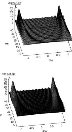
Figure 1 illustrates the rate of absorption changing upon change of time, whenν = 2.5. We see that the spectrum changes from a Lorentzian shape centered atω=ω0to a bi-modal shape at later time, in accordance with earlier theoret-ical work [24, 25]. The authors of Ref. [24] studied the aged conditionf(t,∞)with2 < ν <3, and found that the cor-responding spectrum has two sharp peaks. Klafter and Zu-mofen proved that the same case withf(t, ta = 0) =ψ(t)
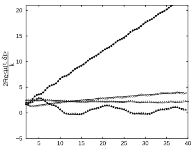
yields L´evy diffusion, thereby implying an exponential char-acteristic function, and consequently a Lorentzian spectrum. It is remarkable that our theoretical perspective establishes a connection between the prediction of Zumofen and Klafter, valid at short times, and that of Ref. [24], valid at large times. Remarkably, we evaluate numerically also the spec-trum time evolution in the caseν < 2, where the process of aging keeps going on forever without ever reaching the stationary condition, which does not exist, in this case (see Fig. 2).
5
Theoretical calculations
Let us show now how to reproduce these numerical results with a proper theoretical treatment. Let us consider as an example a single trajectory starting a timet′withξ= +W and ending at time t with the same positive value aftern
switches of the variableξbetween its two values±W. In this case the integrand of (14), has the following form:
exp[α+(t1−t′) +α−(t2−t1) +...+α+(t−tn)] (17)
whereα± =i(δ±W)andncan only be even.
To determine the contribution tohµ(t)iof Eq. (15) stem-ming from this kind of trajectories, we have to average the term (17) on the set of all possible sequences of the variable
ξ(t)running fromt′totwithnswitches, to sum overnand then to carry out the integration ont′.
δ/W
-1 -0.5 0
0.5 1
5 10 15 20 25 30 35 40
Wt 0 1 2 3 4 5 2Re<µ(t,δ)>
k
δ/W
-1 -0.5 0
0.5 1
5 10 15 20 25 30 35 40
Wt 0 1 2 3 4 5 2Re<µ(t,δ)>
k
Figure 1. The numerical (top) versus the theoretical (bottom) ab-sorption spectrum withν = 2.5,T ·W = 0.4. We assign to the fluctuationξ(t)the intensityW = 1.
k
2
Z t 0
dt′ Ã
F(t−t′, t′)eα+(t−t′)+
∞ X
n=1 Z t
t′
dt1f(t1−t′, t′)
·eα+(t1−t′)
Z t
t1
dt2ψ(t2−t1)eα−(t2−t1) Z t
t2
dt3ψ(t3−t2)
·eα+(t3−t2)· · ·
Z t
t2n−1
dt2nψ(t2n−t2n−1)eα−(t2n−t2n−1)
·Ψ(t−t2n)eα+(t−t2n)
!
,
(18) where, in addition to the crucial probability densityf(τ, t′), we have used
Ψ(τ) = 1−
Z τ 0
ψ(τ′)dτ′, (19)
which is the conventional probability that no switch occurs for a generic interval of timeτ, and
F(τ, t′) = 1− Z τ
0
f(τ′, t′)dτ′, (20)
δ/W
-1 -0.5 0
0.5 1
5 10 15 20 25 30 35 40
Wt -50
5 10 15 20 25 2Re<µ(t,δ)>
k
δ/W
-1 -0.5 0
0.5 1
5 10 15 20 25 30 35 40
Wt -50
5 10 15 20 25 2Re<µ(t,δ)>
k
Figure 2. The numerical (top) versus the theoretical (bottom) ab-sorption spectrum withν= 1.5,T ·W = 0.4. We assign to the fluctuationξ(t)the intensityW = 1.
which is the corresponding aging property, depending on
f(τ, t′), and indicating therefore the conditional probability that, fixedt′, no switch occurs betweent=t′andt=t′+τ. The overall factor of1/2 of the contribution (18) is a con-sequence of the fact that at timet′the fluctuationξ(t), sup-posed to be positive, can get with the same probability the negative value. Let us address now the problem of finding an exact analytical expression for the crucial propertyf(τ, t′). The exact expression forf(τ, t′), is
f(τ, t′) =Z
t′ 0
dτ′G(t′−τ′)ψ(τ+τ′), (21)
where
G(t)≡δ(t) +ψ(t) +
∞ X
n=2 Z t
0
dt1ψ(t1) (22)
·
Z t
t1
dt2ψ(t2−t1)... Z t
tn−2
dtn−1ψ(t−tn−1).
It is straightforward to find the Laplace transform ofG(t). This is given by
ˆ
G(u) =
∞ X
n=0
ˆ
ψ(u)n = 1
whereψˆ(u)denotes the Laplace transform ofψ(t). Thus, the Laplace transform of (21) with respect tot′reads:
ˆ
f(τ, u′) = 1 1−ψˆ(u′)e
u′τ
·
ˆ
ψ(u′)−
Z τ 0
e−u′yψ(y)dy
¸
,
(24) thereby yielding:
f(τ, t′) =L−1[ ˆf(τ, u′)]. (25) where the double Laplace transform, after some algebra, reads
ˆ
f(u, u′) = ψ(u′)−ψ(u)
(u−u′)[1−ψ(u′)]. (26) With this expression the prescription necessary to evaluate the contribution tohµ(t)iof Eq. (15) of the trajectories be-ginning in the “light on” state att′ and ending in the same state att, is completed.
As a last step, we calculate the Laplace transform of (18), and of the equivalent expressions for all the other pos-sible conditions of motion from t′ to t, namely, with the noiseξ(t)moving from+Wto−W, from−W to+Wand, finally, from −W to−W, as well. This procedure yields, as a final result, the Laplace transform ofR(t), denoted by
ˆ
R(u), which is proved to have the following analytical ex-pression:
ˆ
R(u) =kL[hµ(t)+µ∗(t)i] = k
2
2 (A+(u)+A−(u)+C(u)).
(27) The explicit expression forA+(u), which is calculated tak-ing into account the contribution tohµ(t)iof those trajecto-ries ending at timetwith a positive valueξ(t) = +W for the flucuating variable, is
A+(u)≡
ˆ
Ψ(u−α+)[ ˆf+(u) ˆψ(u−α−) + ˆf−(u)]
1−ψˆ(u−α+) ˆψ(u−α−)
+ ˆF+(u),
(28) with:
ˆ
Ψ(u−α±) =L[Ψ(t)eα±t] =
1−ψˆ(u−α±)
u−α±
, (29)
ˆ
f±(u) ≡ L ·Z t
0
dt′f(t−t′, t′)eα±(t−t′)
¸ (30)
= ψˆ(u)−ψˆ(u−α±) −α±(1−ψˆ(u))
and
ˆ
F±(u)≡ L ·Z t
0
dt′F(t−t′, t′)eα±(t−t′) ¸
= 1/u−fˆ±(u) (u−α±)
.
(31)
A−(u)takes into account the contribution of all trajectories ending at timet with the negative valueξ(t) = −W, for the fluctuating variable and is derived from the expression for A+(u)by replacing everywhere α± withα∓ (sending
ˆ
f±,Fˆ± → fˆ∓,Fˆ∓). Thus, k(A+(u) +A−(u))/2 repre-sents the laplace transform ofhµ(t)i. FinallykC(u)/2 is
the Laplace transform ofhµ∗(t)i, and it is derived from the earlier expression fork(A+(u) +A−(u))/2 by replacing everywhereα±with−α±. To establish a comparison with the result of the numerical experiment we have anti-Laplace transformed the analytical expression of Eq. (27) using a Talbot algorithm implemented on Mathematica 5.0. The re-sult of this procedure is illustrated by both Fig. 1 and Fig. 2, where the analytical predictions are compared to the cor-responding numerical experiments. The overall qualitative agreement is remarkably good. Apparently, in Fig. 1 the de-parture of the theoretical calculation from the fine structure of the numerical result is larger than in Fig. 2. Actually, the numerical algorithm produces fluctuations of the same intensity in both cases, although the more detailed scale of Fig. 1 makes them appear larger. To establish beyond any doubt also the quantitative agreement, in Fig. 3 we compare the two predictions for specific values of the de-tuning para-meterδ. This shows that also the quantitative agreement is very satisfactory. Furthermore, when a stationary condition exists, it is straightforward to prove that Eq. (27) recovers, as asymptotic-time limit, the same result as that of [6].
5 10 15 20 25 30 35 40
−5 0 5 10 15 20
<µ(
2Re
t,
W
δ)>
k
t
Figure 3. Comparison between numerical and theoretical absorp-tion spectra for different values of the de-tuning parameterδand of the power indexν. Moving from the top to the bottom in the right hand portion of the figure,δ= 1,ν = 1.5,δ= 1,ν= 2.5,
δ = 0.6,ν = 2.5,δ = 0.6,ν = 1.5. The numerical curves are denoted by black circles, open circles, open triangles and black tri-angles, respectively, and in this scale are almost indistinguishable from the full lines denoting the corresponding theoretical results.
6
Conclusions
We have adopted a procedure based on the observation of single trajectories, along the lines of the pioneering work of Montroll and Weiss on the Continuous Time Random Walk (CTRW) [26]. Rather than building up a master equation, we have studied the action of the radiation field on the sin-gle diffusional trajectory. Note that the field acting at time
the procedure here adopted, yields Eq. (15), with the sub-script t′ working as an age indicator. This formula inter-twines the system to the radiation field, thereby violating the ordinary linear response prescription, which is recovered in fact in the Poisson case. The breakdown of the linear re-sponse theory is a manifestation of the failure of the den-sity method. A GME, of whatsoever origin, including that generated by the condition of being totally equivalent to the CTRW [27], always incorrectly responds to an external per-turbation, as a consequence of missing, by its very nature, the entanglement with the external perturbation. It is im-portant to notice that the breakdown of the density approach method has been independently observed by Sokolov, Blu-men and Klafter [28]. These authors have built up a Fokker-Planck (FP)-like equation that should be equivalent to the CTRW of a given age (the brand new age, in their case). The action at later times of an external perturbation on this FP equation yields result that are distinctly different from those obtained by adopting the single trajectory picture with the external trajectory acting on the single unperturbed tra-jectory.
It is important to stress that we have adopted a vision corresponding to assuming the wave-function collapses to really occur. It is well known, in fact, that according to de-coherence theory [29] the wave-function collapse is mim-icked by a density matrix becoming diagonal in the basis set of the eigenstates of the variable that is measured [30]. This approach implies the adoption of a reduced density matrix, and consequently of the GME that one can derive from a Liouville equation, via the adoption of a convenient projec-tion method (see, for instance, Ref. [31]). We have adopted, on the contrary, a picture based on the assumption of the existence of real trajectories. It is of fundamental impor-tance at this stage to assess whether an equivalent Liouville or Liouville-like approach can be used, to yield the same result. The arguments of Section 2 seem to rule out this pos-sibility.
GA and PG thankfully acnowledge ARO and Welch Foundation for financial support through Grant DAAD19-02-1-0037 and 70525, respectively .
References
[1] R. Kubo, J. Phys. Soc. Japan 9, 935 (1954); Adv. Chem. Phys.15, 101 (1969); P.W. Anderson, J. Phys. Soc. Jpn.9, 316 (1954).
[2] R. G. Neuhauser, K. T. Shimizu, W. K. Woo, S. A. Empedo-cles, and M. G. Bawendi, Phys. Rev. Lett.85, 3301 (2000). [3] M. Kuno, D.P. Fromm, H. F. Hamann, A. Gallagher, and D.J.
Nesbitt, J. Chem. Phys.112. 3117 (2000).
[4] X. Brokmannet al, Phys. Rev. Lett.90, 120601 (2003).
[5] P. Allegrini, G. Aquino, P. Grigolini, L. Palatella, and A. Rosa, Phys. Rev.68, 056123 (2003).
[6] Y.-J. Jung, E. Barkai, R. J. Silbey, Chem. Phys. 284, 181 (2002).
[7] . D.R. Cox, Renewal Theory, Chapman and Hall, London (1962).
[8] P. Allegrini, G. Aquino, P. Grigolini, L. Palatella, A. Rosa, and B. J. West, arXiv:cond-mat/0409600.
[9] C. Beck, Phys. Rev. Lett.87, 180601 (1-4) (2002).
[10] C. Tsallis, J. Stat. Phys.52, 479 (1988).
[11] C. Beck, E.G.D. Cohen, Physica A322, 267 (2003).
[12] C. Beck, Physica A342, 139 (2004).
[13] M. Bologna, P. Grigolini, M. G. Pala, L. Palatella, Chaos, Solitons & Fractals,17, 601 (2003).
[14] P. Grigolini, Chem. Phys.38, 389 (1979).
[15] P. Allegrini, P. Grigolini, L. Palatella, and B. J. West, Phys. Rev. E70, 046118 (2004).
[16] G. Aquino, M. Bologna, P. Grigolini, and B. J. West, Phys. Rev. E70, 036105 (2004).
[17] P. Grigolini, submittted to Physica A.
[18] R. Veberk, A. M. van Ojien, and M. Orrit, Phys. Rev. E B66, 233202 (2002).
[19] J.P. Bouchaud, J. Phys. I (France)2, 1705 (1992).
[20] J. P. Bouchaud and D.S. Dean, Aging on Parisi’s Tree, J. Phys. I France5, 265 (1995).
[21] G.M. Zaslavsky, Phys. Rep.371, 461 (2002).
[22] Y.-J. Jung, E. Barkai, and R. Silbey, Adv. Chem. Phys.123, 199 (2002) (see also: arXiv::cond-mat/0311428).
[23] E. Barkai, Phys. Rev. Lett.90, 104101 (2003).
[24] P. Allegrini, P. Grigolini, B.J. West, Phys. Rev. E54, 4760 (1996).
[25] J. Klafter, G. Zumofen, Physica A,196, 102 (1993).
[26] E.W. Montroll and G.H. Weiss, J. Math. Phys.6, 167 (1965).
[27] V. M. Kenkre, E.W. Montroll, and M.F. Shlesinger, J. Stat. Phys.9, 45 (1973).
[28] I.M. Sokolov, A. Blumen and J. Klafter, Europhys. Lett.56, 175 (2001).
[29] H.D. Zeh, Found. Phys.1, 69 (1970).
[30] Z.H. Zurek, Phil. Trans. Roy. Soc. Lond. A356, 1793 (1998).