Controlling the depth of anesthesia by a novel positive control strategy

Controlling the depth of anesthesia by a novel positive

control strategy

F. N. Nogueiraa,b_{, T. Mendon¸ca}c,b_{, P. Rocha}a,b

a_{Faculdade de Engenharia da Universidade do Porto, Porto, Portugal.}

b_{CIDMA - Center for Research and Development in Mathematics and Applications,}

Department of Mathematics, University of Aveiro, Portugal.

c_{Faculdade de Ciˆencias da Universidade do Porto, Porto, Portugal.}

Abstract

In this paper a positive control law is designed for multi-input positive systems that ensures asymptotic tracking of a desired output reference value. This control law can be viewed as a generalization of another one proposed in the literature for the control of the total mass in SISO compartmental systems, but is suitable for a wider class of positive systems. The controller proposed here is applied to the control of the depth of anesthesia (DoA), by means of the administration of propofol and remifentanil, when using a parameter parsimonious Wiener model recently introduced in the literature. Its performance is illustrated by realistic simulations.

Keywords:

I_{This work was supported by FEDER founds through COMPETE–Operational} Pro-gramme Factors of Competitiveness (“Programa Operacional Factores de Competitivi-dade”) and by Portuguese funds through the Center for Research and Development in

Mathematics and Applications (University of Aveiro) and the Portuguese Foundation for

Science and Technology (“FCT–Funda¸c˜ao para a Ciˆencia e a Tecnologia”), within project PEst-C/MAT/UI4106/2011 with COMPETE number FCOMP-01-0124-FEDER-022690. The authors also acknowledges GALENO - Modeling and Control for personalized drug ad-ministration, Funding Agency: FCT,Programme: FCT PTDC/SAU-BEB/103667/2008. Additionally, Filipa Nogueira acknowledges the support of FCT - Portugal through the grant SFRH/BD/48314/2008.

Please cite this article as: F.N. Nogueira, et al., Controlling the depth of anesthesia by a novel positive control strategy, Comput. Methods Programs Biomed. (2014), http://dx.doi.org/10.1016/j.cmpb.2013.12.016

Positive systems, control, DoA, anesthesia. 1. Introduction

The goal of automatically controlled drug administration is to determine the dosage to be administered to achieve and keep a certain effect of a drug in the patient. In this work, the primary goal is to track the level of the depth of anesthesia, here measured by the bispectral index (BIS), which is trans-formed into a problem of tracking the effect concentration by inverting the generalized Hill equation. This problem can be modeled as an output refer-ence tracking problem. More specifically, after modeling the phenomenon in question by a control system in which the control input is the dosage of drug to be administered and the output is the corresponding effect, one seeks a control law that forces the system output to converge to the desired reference value.

Since the quantities involved in this process are all nonnegative, this prob-lem falls within the realm of positive systems. These systems have gained increasing attention in the control literature during the last decades. See for example Farina and Rinaldi [1], Haddad et al. [2], Roszak and Davison [3], Roszak and Davison [4],Kaczorek [5], Willems [6], Soltesz et al. [7]. In this latter reference, a controller by integral action together with a positivity constraint was proposed, showing that the input is positive provided that the integral gain ‘ > 0 is chosen sufficiently small. This controller does not presuppose a full knowledge of the model, however it does need the a pri-ori knowledge of the steady-state gain matrix, in order to obtain a suitable value for the integral gain ‘. This may take a long time to obtain in case the

process poles are not fast enough. This constitutes a disadvantage for its use in our application. The controller presented in this paper ensures reference tracking independently from the positive value of the design parameter, with-out requiring the knowledge of the steady-state gain matrix. Nevertheless, it does require information about the model parameters and the corresponding state. However, these parameters can be identified in a short preliminary stage, and a state observer can be included in order to estimate the state online. The control law, developed in this work, is considered to be nonlin-ear, not due to use of nonlinear design methods, but rather because of the imposition of positivity constraint on the control variable, which makes it a nonlinear function of the state of the system.

In this paper we consider single output positive systems with multiple inputs and design a nonlinear positive control law that ensures asymptotic tracking of a desired output reference value. This control law can be viewed as a generalization of the one proposed in Bastin and Provost [8] for the control of the total mass in SISO compartmental systems. However, whereas the control law in Bastin and Provost [8] is only designed for compartmental systems, our control law is suitable for a wider class of positive systems as is sustained by the new theoretical results presented in the paper (Section 2).

Our results prove to be useful for the control of the depth of anesthesia, a problem that has lately deserved much attention. For instance, the work developed in Soltesz et al. [7] presents two controllers in parallel for the DoA of a patient based on a PID controller for the administration of propofol and a proportional controller for the input of remifentanil. Here, we present one single multi-output feedback controller for both drugs. A good overview of

the underlying problem may be found in Dumont [9] and in the references there in.

The proposed controller is applied to the control of the depth of anesthesia by means of propofol and remifentanil using the recently proposed parameter parsimonious Wiener model (see Silva et al. [10]). The performance of the controller is analyzed by means of several simulations along with realistic simulations relying on identified real patients data collected in the surgery room during general anesthesia.

The present paper is structured as follows. In Section 2 a control law is designed for output reference tracking in MISO positive systems. The application of the corresponding controller in general anesthesia is presented in Section 3. In Section 4 the performance of the proposed controller is illustrated by means of several simulations, and the results of its application in realistic simulated patients are presented in Section 5. Conclusions follow in Section 6.

2. Output Reference Tracking for MISO Positive Systems

In this section the general problem of reference tracking for multi-input/single-output (MISO) positive systems is presented. The application to the control of anesthesia will be presented in Section 3.

2.1. Problem Description

Consider a positive system with m inputs and a single output described by the state-space model

Y _ ] _ [ ˙x(t) = Ax(t) + Bu(t) y(t) = Cx(t), (1)

where A is a n ◊n Meztler matrix, i.e., a matrix in which all the off-diagonal components are nonnegative, and B and C are matrices with nonnegative entries (see Godfrey [11]) of dimension n ◊ m and 1 ◊ m, respectively. Here, for short, in the sequel (1) is denoted by (A, B, C). Moreover, for a vector

v, the notations v Ø 0 (v > 0) and v Æ 0 (v < 0) mean that all its entries are

respectively positive (strictly positive) and negative (strictly negative). The same applies to matrices.

Given a desired constant reference value yú for the output, a control law

u= Kx + L is sought such that the closed-loop system

Y _ ] _ [ ˙x(t) = (A + BK)x(t) + BL y(t) = Cx(t), (2)

has bounded trajectories and tracks the reference, i.e., such that its output verifies limtæŒy(t) = yú.

2.2. Controller design

Here we solve the problem of output reference tracking, by regarding it as a problem of controlling the system to a level set yú= {x œ Rn₊: Cx = yú}

in the state space, where Rn

+= {x œ Rn : x Ø 0}.

For this purpose, we first design an auxiliary control law, ˜u, and then impose positivity to ˜u in order to obtain a positive control input u. We also make the following assumptions: (A1) A is stable, (A2) CB is a nonzero row matrix and (A3) CA < 0.

Let

˜u(t) = ≠ECAx(t) + E⁄(yú_{≠ y(t)), (3)}

where ⁄ > 0 is a design parameter, and E is a column matrix with nonnega-tive entries such that CBE = 1. Note that such a matrix always exists since

CB has nonnegative entries, at least one of each is strictly positive. The

application of this control input leads to the closed-loop dynamics

˙x(t) = Ax(t) + B(E⁄(yú_{≠ y(t)) ≠ ECAx(t)) (4)}

which implies that

˙y(t) = C ˙x(t) = CAx(t) + ⁄(yú_{≠ y(t)) ≠ CAx(t) (5)}

= ≠⁄(y(t) ≠ yú_{) (6)}

and therefore

˙

‰

y(t) ≠ yú = ≠⁄(y(t) ≠ yú). (7)

Hence, y(t) ≠ yú _{= e}≠⁄t_{(y(0) ≠ y}ú_{) and}

lim

tæŒy(t) = y

ú_{, (8)}

which means that the output reference value is asymptotically tracked. In the sequel it is shown that reference tracking can still be achieved even when a positivity restriction to the control input is imposed. This positivity restriction is made componentwise and corresponds to taking the control input as u = 5 u1 · · · um

6T

with ui = max(˜ui,0), where ˜ui denotes the i≠ th component of ˜u. Note that ˜ui = Ei(≠CAx + ⁄(yú≠ y)), where EiØ 0

is the i ≠ th entry of E. Therefore if ˜ui< 0 then ≠CAx + ⁄(yú≠ y) < 0, and

all the other components ˜uj of ˜u corresponding to nonzero Ej are negative

as well. This allows to conclude that either u = ˜u or u = 0. In this latter case

⁄(yú≠ y) < CAx. (9)

Since, by assumption (A3), CA < 0 and x Ø 0, then CAx Æ 0 and (9) implies that yú_{≠ y < 0.}

To prove that all trajectories converge to yú, we apply the LaSalle’s

in-variance principle (see LaSalle [12], Leine and Wouw [13], Liao et al. [14], Bullo [15]) to the Lyapunov function

V(x) = 1

2(yú≠ y)2 (10)

for the system (1) on Rn

+.

For u = ˜u:

˙V (x) = ≠(yú_{≠ y) ˙y = ≠(y}ú_{≠ y)C ˙x (11)}

= ≠(yú_{≠ y)C (Ax + B [E⁄(y}ú_{≠ y) ≠ ECAx]) (12)}

= ≠⁄(yú_{≠ y)(y}ú_{≠ y) = ≠⁄(y}ú_{≠ y)}2 _{Æ 0 (13)}

For u = 0 (which can only happen when yú_{≠ y < 0, see (3)):}

˙V (x) = ≠(yú_{≠ y)C ˙x = ≠ (y}ú_{≠ y)} ¸ ˚˙ ˝ <0 CAx ¸ ˚˙ ˝ Æ0 Æ 0 (14)

Thus ˙V (x) = Y _ ] _ [

≠⁄(yú_{≠ y)}2 for u = ˜u

≠(yú_{≠ y)CAx for u = 0} (15)

By the LaSalle’s invariance principle, all system trajectories converge to the largest set contained in

W = {x œ Rn

+: ˙V (x) = 0}, (16)

which is forward-invariant under the closed-loop dynamics. It follows from (15) that ˙V (x) = 0 either when u = ˜u and y = yú or when u = 0,which

implies yú_{< y}, and CAx = 0. So we get

W = {x œ Rn₊: y = yú or (yú< y and CAx = 0)}. (17)

Moreover, the set yú of positive states for which the corresponding

out-put y equals yú is forward-invariant under the closed-loop dynamics. In fact,

let F (x) be the vector field associated with the closed-loop system

Y _ ] _ [ ˙x = Ax + Bu u= max(˜u, 0). (18)

When Cx = yú, u = ˜u = ≠ECAx Ø 0 and F(x) = Ax ≠ BECAx. As a

consequence, recalling that CBE = 1, one obtains CF (x) = 0 showing that

F(x) is tangent to yú. So _yú is forward-invariant under the closed-loop

dynamics.

On the other hand, the trajectories starting in a state x for which Cx > yú

Cx > yú ∆ u = 0 (19)

∆ ˙x(t) = Ax(t). (20)

Since A is assumed to be stable, if the control would remain zero, then limtæŒCx(t) would be zero. This implies that at a certain time instant,

say tú, Cx(tú) reaches the value Cx(tú) = yú, i.e. x(tú) œ

yú. From this

instant on the trajectories remain indefinitely in the forward-invariant set

yú. Therefore, the largest invariant subset contained in W is _yú and, by

LaSalles’s invariance principle, all the closed-loop system trajectories con-verge to this set, which means that limtæŒy(t) = yú as desired.

The study just developed leads to the following result.

Theorem 1. Let (A, B, C) be a positive MISO linear system, such that A

is stable, CA < 0 and CB ”= 0. If u = max(˜u, 0), ˜u = ≠ECAx + E⁄(yú_≠

y), with ⁄ > 0, and E Ø 0 such that CBE = 1, then the closed-loop system

output y(t) verifies limtæŒy(t) = yú.

3. CONTROL OF THE DEPTH OF ANESTHESIA

Combinations of drugs are used in general anesthesia because no single drug is able to provide all its necessary components (namely, analgesia, hyp-nosis, areflexia) without seriously compromising hemodynamic and/or res-piratory function, impairing operating conditions, or delaying postoperative recovery. Ideal combination of dosing facilitates optimal therapeutic effect without producing significant side effects.

Here, a control law is designed to administer the hypnotic agent propofol and the opioid analgesic remifentanil to patients during surgery, in order to achieve a desired level of unconsciousness. This is measured in terms of the depth of anesthesia (DoA), usually denoted by z(t), which is a feature that can be related to the quantities of administered drugs as explained next.

In what concerns DoA, the response to the administration of hypnotics and analgesics is commonly modeled as a high order pharmacokinetic/phar-macodynamic (PK/PD) Wiener model (see Bailey and Haddad [16]). How-ever, a new Wiener model (parameter parsimonious Wiener model) with a reduced number of parameters describing the join effect of propofol and of

remifentanil as been introduced in Silva et al. [10]. Here, the main goal of

this section is to design a controller for the DoA based on this parameter parsimonious Wiener model.

The effect concentration of propofol (cp

e) and of remifentanil (cre) can be

modeled by the parameter parsimonious Wiener model developed by Silva et al. [10]. According to this model

cp e(s) = k1k2k3–3 (k1–+ s)(k2–+ s)(k3–+ s)u p(s), (21) cr_e(s) = l1l2l3÷ 3 (l1÷+ s)(l2÷+ s)(l3÷+ s)u r(s), (22) where cp

e(s), cre(s) denote the Laplace transforms of cpe(t) and cre(t),

respec-tively, and up(s) and ur(s) are the Laplace transforms of the administered

the transfer functions in (21) and (22) has three aligned poles, more con-cretely, the first one has poles (≠k1,≠k2,≠k3)– and the second one has poles

(≠l1,≠l2,≠l3)÷. The parameters kj, lj, j = 1, 2, 3 were chosen in Silva et al.

[10] according to the collected patient data and fixed at the values k1 = 10,

k₂ = 9, k₃ = 1, l₁ = 3, l₂ = 2, l₃ = 1. The parameters – and ÷ are patient

dependent.

The joint effect of the concentrations of propofol and remifentanil on the BIS level is modelled in Silva et al. [10] by the generalized Hill equation:

z(t) = z0

1 + (µUp+ Ur)“, (23)

where µ, “ are patient dependent parameters, z0 is the effect at zero

con-centration, and Up and Ur respectively denote the potencies of propofol and remifentanil, which are obtained by normalizing the effect concentrations

with respect to the concentrations that produce half the maximal effect when the drug acts isolated (denoted by ECp

50 and EC50r, respectively), i.e.:

Up= cpe EC₅₀p and Ur = cr e ECr 50. (24)

In this work we consider – œ [0.03 , 0.17], ÷ œ]0 , 5.70], ECp

50 = 10 and

ECr

50 = 0.01. The values of EC50p = 10 and EC50r = 0.01 are taken from

Mendon¸ca et al. [17] and the intervals for the values of – and ÷ are obtained as follows: – œ [¯– ≠ 2‡– , ¯– + 4‡–] and — œ]0 , ¯— + 4‡—], where ¯– and ‡– respectively denote the mean and standard deviation of the parameters

now for the parameter ÷. The choice of lower bound 0 for ÷ is due to the fact that ÷ should be positive and ¯÷ ≠ 2‡÷ <0.

The transfer functions in (21) and (22) can be represented by the follow-ing state-space model:

Y _ ] _ [ ˙xi = Ai_xi+ Bi_ui ci e= 5 0 0 1 6xi_{, i}= p, r (25) where xi = S W W W W W U xi 1 xi 2 xi 3 T X X X X X V is the state, Ap = S W W W W W U ≠10– 0 0 9– ≠9– 0 0 – ≠– T X X X X X V , Ar = S W W W W W U ≠3÷ 0 0 2÷ ≠2÷ 0 0 ÷ ≠÷ T X X X X X V , Bp = S W W W W W U 10– 0 0 T X X X X X V and Br= S W W W W W U 3÷ 0 0 T X X X X X V . (26)

Defining U = µUp+ Ur yields

with U = 1 EC₅₀p µc p e+ 1 ECr 50c r e = 0.1µcpe+ 100cre. (28)

This leads to the following model

Y _ _ _ _ _ ] _ _ _ _ _ [ ˙x(t) = Ax(t) + Bu(t) U(t) = 0.1µcp e(t) + 100cre(t) = Cx(t) z(t) = z0 1+U“, (29) where x(t) = S W U x p(t) xr(t) T X V, A= S W U A p 0 3◊3 0_3◊3 Ar T X V, B = S W U B p 0 3◊1 0_3◊1 Br T X V, C = 5 0 0 0.1µ 0 0 100 6. (30)

As mentioned before, for surgery purposes it is desirable to maintain the BIS close to a certain reference level zref between 40 and 60. This can be

achieved by designing a control law that forces U(t) to follow the constant reference level

Uref = “

Ú _z

0

zref ≠ 1. (31)

In order to apply the design method of the previous subsection, the prod-uct CB should be a nonzero row. However, here CB = 5 0 0 6 and the

condition is not met. To overcome this problem, instead of the output U(t), the output M(x(t)) = 0.1Mp(xp(t)) + 100Mr(xr(t)) = CMx(t), (32) with Mp(xp) =5 _{1 1 1} 6_xp_{, M}r(xr) =5 _{1 1 1} 6_xr and CM = 5 0.1 0.1 0.1 100 100 100 6, (33)

is considered. The notations M(x(t)), Mp(xp(t)), and Mr(xr(t)) are inspired

by the fact that, in compartmental systems, the sum of the state components usually corresponds to the total substance mass present in the system. As we shall later see, a connection between the reference value Uref and an adequate

reference value Mref for M can be established, in such a way that when

limtæŒM(x(t)) = Mref then limtæŒU(t) = Uref and limtæŒz(t) = zref, as

desired.

In a first stage we show that every positive constant reference value Mú

for M (x(t)) can be tracked using a control law as proposed in Theorem 1. Then, in a second step, we determine which value should be taken for Mú

in order to ensure that the desired constant reference value zref for the BIS

level is achieved.

Since now, for the new output matrix CM, defined in (33), CMB =

5

– 300÷

6

is nonzero, the applicability of the proposed controller design method is guaranteed.

Proposition 1. Let (A, B, CM) be a positive MISO linear system, with A, B as in (30) and CM as in (33). Define E = S W U fl 1 T X V_{–fl+ 300÷}1 , (34)

where fl > 0 is an arbitrary nonnegative value. Then, applying the control law u= max(0, ˜u), (35) with ˜u = S W U ˜u p ˜ur T X V= E (≠CMAx+ ⁄(Mú≠ M)) and ⁄ > 0 (36) = S W U fl 1 T X V(≠CMAx+ ⁄(Mú≠ M)) 1 –fl+ 300÷ ¸ ˚˙ ˝ ¯u , (37) and ⁄ > 0

to the system (A, B, CM), yields limtæŒM(x(t)) = Mú.

Proof. Since CMBE = 1, all the conditions of Theorem 1 are satisfied

yield-ing the desired result.

Remark: Note that, in this control law, ⁄ and fl are design parameters. Moreover S W U ˜u p ˜ur T X V= S W U fl 1 T X

V¯u, with ¯u as in (37), meaning that the proportion

of propofol and remifentanil is fl : 1.

Since the choice of the positive parameter fl does not affect the tracked reference value, this may constitute an advantage, as it allows to choose

the proportion between the two drugs, in order to accommodate clinical restrictions or considerations, without significant consequences in terms of the effect. This will be illustrated later on in the simulations.

In order to determine which value of Mref should be chosen for Mú in

the control law (37) to guarantee that the BIS level z(t) tracks a desired constant value zú, an analysis is made of the values U(t) obtained for the

closed-loop system. For this purpose it will be first proved that the state of the closed-loop system (A, B, CM) with the control law (35) converges to

an equilibrium point xú. To show this, since, as mentioned in the previous

section, the trajectories x(t) converge to the forward-invariant set Mú =

{x œ R6+ : M(x) = Mú}, it is enough to prove that, for the restriction

of the closed-loop system to this set, the state trajectories converge to an equilibrium point xú. Note that this restriction is well defined as

Mú is

forward-invariant under the closed-loop dynamics.

In order to obtain the dynamics of the system restricted to Mú, note that

when x œ Mú, i.e., when M(x) = Mú, the control ˜u is given by ˜u = ≠ECAx,

and the closed-loop system can be described as

˙x = ˜Ax (38)

˜ A = A ≠ BECMA = S W W W W W W W W W W W W W W W U a1≠ 10– 8a1 a1 a2 a2 a2 9– ≠9– 0 0 0 0 0 – ≠– 0 0 0 a3 8a3 a3 a4≠ 3÷ a4 a4 0 0 0 2÷ ≠2÷ 0 0 0 0 0 ÷ ≠÷ T X X X X X X X X X X X X X X X V where a1 = –2fle, a2 = 1000–÷fle, a₃ = 0.3–÷e, a₄ = 300÷2e, e= _–fl+300÷1

and A, B, CM and E are given by (30), (33), and (34).

In order to analyze the stability of the closed-loop system restricted to

Mú, the evolution equations of this restriction are next obtained.

When M(x(t)) = Mú_,

xp₁(t) = Mú≠ xp2(t) ≠ xp3(t) ≠ 1000(xr1(t) + xr2(t) + xr3(t)). (39)

Y _ _ _ _ _ _ _ _ _ _ _ _ _ _ _ _ _ _ _ ] _ _ _ _ _ _ _ _ _ _ _ _ _ _ _ _ _ _ _ [ ˙xp 1(t) = Mú≠ ˙xp2(t) ≠ ˙xp3(t) ≠ ˙xr1(t) ≠ ˙xr2(t) ≠ ˙xr3(t) ˙xp 2(t) = 9–(Mú≠ xp2(t) ≠ xp3(t) ≠ 1000(x1r(t) + xr2(t) + xr3(t))) ≠ 9–xp2(t) ˙xp 3(t) = –xp2(t) ≠ –xp3(t) ˙xr 1(t) = a3Mú+ 7a3x2p(t) + (a4≠ 1000a3≠ 3÷)xr1(t)+ +(a4≠ 1000a3(xr2(t) + xr3(t)) ˙xr 2(t) = 2÷xr1(t) ≠ 2÷xr2(t) ˙xr 3(t) = ÷xr2(t) ≠ ÷xr3(t). (40)

Since the state component xp

1(t) can be obtained from the others state

com-ponents (see (39)), we can conclude that the closed-loop system dynamics restricted to Mú is described by the evolution of the vector

¯x = S W W W W W W W W W W W W U xp₂ xp₃ xr 1 xr 2 xr 3 T X X X X X X X X X X X X V , (41)

which is given by the last five equations from (40). These equations can be written in matrix form as:

with ¯ A= S W W W W W W W W W W W W U ≠18– ≠9– ≠9000– ≠9000– ≠9000– – _≠– 0 0 0

7a3 0 a4≠ 1000a3≠ 3÷ a4≠ 1000a3 a4≠ 1000a3

0 0 2÷ ≠2÷ 0 0 0 0 ÷ _≠÷ T X X X X X X X X X X X X V and R= S W W W W W W W W W W W W U 9–Mú 0 a₃Mú 0 0 T X X X X X X X X X X X X V .

Moreover, equation (42) can be written in the form: ˙ ‰ ¯x ≠ ¯xú_{= ¯A(¯x ≠ ¯x}ú_{), (43)} where ¯xú ₌ S W W W W W W W W W W W W U fl fl 1 1 1 T X X X X X X X X X X X X V Mú 3(0.1fl + 100) (44)

is the only equilibrium point of (42), i.e., the only point such that ¯x(t) © ¯xú

satisfies ˙¯x = ¯A¯x(t) + R, as ˙¯x(t) = 0 and ¯A¯xú= ≠R. This can be verified by

equals ≠R. Moreover, the uniqueness of ¯xú follows from the invertibility of

¯

Afor the considered parameter range.

As is shown in Fig. 1, where the locations of the eigenvalues of ¯A are

plotted for the different value combinations of the parameters – and ÷, within the ranges in this paper, and for fl œ [0 , 500], the matrix ¯A is stable, i.e.,

all its eigenvalues have negative real part. The restriction fl œ [0 , 500] is only imposed to limit the high computation level, however this feat is not a limitation to the applicability of the controller here proposed, since the fl values observed in the collected clinical cases are included in the considered interval. Thus, ¯x(t) converges to ¯xú = (fl, fl, 1, 1, 1) Mú

3(0.1fl+100). Recalling that

equation (39) holds, this implies that x(t) = (xpú

1 , ¯xú) with xp₁ú = Mú≠ 5 1 1 100 100 100 6¯xú ₍₄₅₎ = _{3(0.1fl + 100)}flMú . (46) Thus x(t) converges to xú = (fl, fl, fl, 1, 1, 1) Mú

3(0.1fl+100) under the

Figure 1: Location of the eigenvalues of the matrix ¯A, for the different value combinations

of the parameters –, ÷ and fl within the ranges in this paper, i.e., – œ [0.03 , 0.17],

÷œ]0 , 5.70], fl œ [0 , 500]

Recalling that u(t) = 0.1µxp

3(t) + 100xr3(t), one concludes that, under the

closed loop dynamics,

Uú = lim tæŒU(t) = 0.1µ limtæŒx p 3(t) + 100 lim_tæŒxr3(t) (47) = 0.1µ_{3(0.1fl + 100)}flMú + 100_{3(0.1fl + 100)}Mú (48) = Mú 0.1µfl + 100 3(0.1fl + 100). (49)

Consequently, in order to track a constant reference level Uref for U(t) it

is enough to take

in the control law (35).

Together with expression (31), these considerations lead to the following result.

Proposition 2. Let (A, B, CM) be a positive MISO linear system, with A,

B as in (30) and CM as in (33). Then, applying the control law u as in (35),

with Mú = Mref = 3(0.1fl+100)

0.1µfl+100 “

Ò

z0

zref ≠ 1, to the system (A, B, CM), achieves

tracking of the constant reference value zref for the BIS level z(t) defined as

in (23), i.e., limtæŒz(t) = zref.

Proof. It follows from what has just been said that taking in (35) Mú= Mref = 3(0.1fl + 100)_{0.1µfl + 100} “

Ú _z

0

zref ≠ 1

achieves tracking of the constant reference value for U:

Uref = “

Ú _z

0

zref ≠ 1.

The result now follows from expression (31).

As stated in Proposition 2, once the values of “ and µ are known for a particular patient, the value of Mref to be considered in the control law is:

Mref = 3(0.1fl + 100)_{0.1µfl + 100} “

Ú _z

0

zref ≠ 1, (51)

values of “ and µ are available, however, if this is not the case, these values can be identified in a first stage, before turning on the controller. Another possibility is to start with an average value for “ and µ and hence Mú as a

first estimate and then retune this value after “ and µ are more accurately identified. A similar procedure was used in Nogueira et al. [18]. Here, it is also assumed that the values of the parameters –, ÷ are known. This does not happen in practice. However, in a real situation the controller action only starts after an initial drug bolus is given. This is a current practice with other automatic controllers previously used in clinical environment and allows to identify the parameters for patient model.

4. CONTROLLER PERFORMANCE

In this section the performance of the control law presented in the previ-ous sections is illustrated by means of several simulations. For this purpose, we consider: z0 = 97.7; – = 0.0759; ÷ = 0.583; µ = 1.79; “ = 1.88. These

pa-rameter values are the mean values used in the work developed in Mendon¸ca et al. [17], to which we refer for further explanation. We also assume that it is intended that the DoA of a patient, corresponds to the reference value of 50 for the BIS signal. By (31), this means that U must follow the reference

Uú = 0.9753. Once these values are fixed, the control law only depends on

the design parameters ⁄ > 0 and fl Ø 0. The parameter ⁄ influences the speed of convergence to the reference value, as can be seen in Fig. 2 where the values ⁄ = 0.02, ⁄ = 1 were respectively taken for a fixed value of fl = 2 (corresponding to proportion of 2 : 1 for propofol and remifentanil).

0 2 4 6 8 10 50 55 60 65 70 75 80 85 90 95 100 Time[min] D o A m ea su re m en t (B IS ) λ = 1 λ = 0.02

Figure 2: Evolution of DoA, for fl = 2, ⁄ = 0.02 and ⁄ = 1.

On the other hand the parameter fl specifies the desired proportion be-tween the administered amounts of propofol and remifentanil, which may be chosen according to clinical criteria. Figure 3 illustrates DoA effect for different drug proportions (namely, fl = 0, fl = 2, and fl = 10) and Figures 4, 5, and 6 present the evolution of the corresponding drug dosages. As can be seen in Fig. 3, in spite of the variation of the drug proportion (fl) the desired effect is practically the same. It turns out that this may constitute an advantage, since the choice of the proportion can be made in order to accom-modate individual clinical restrictions or considerations, without significantly consequences in terms of the effect.

0 2 4 6 8 10 50 55 60 65 70 75 80 85 90 95 100 Time[min] D o A m ea su re m en t (B IS ) ρ = 10 ρ = 2 ρ = 0

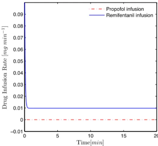
Figure 3: Evolution of DoA for different values of drugs proportion, i.e., fl = 0, fl = 2, fl = 10 and for ⁄ = 1. 0 5 10 15 20 −0.01 0 0.01 0.02 0.03 0.04 0.05 0.06 0.07 0.08 0.09 Time[min] D ru g In fu si o n R a te [mg mi n 1] Propofol infusion Remifentanil infusion

Figure 4: Evolution of the dosage of propofol and of remifentanil, for ⁄ = 1, fl = 0 (without

0 5 10 15 20 0 0.05 0.1 0.15 0.2 0.25 0.3 0.35 Time[min] D ru g In fu si o n R a te [mg mi n 1] Propofol infusion Remifentanil infusion

Figure 5: Evolution of the dosage of propofol and of remifentanil, for ⁄ = 1, fl = 2.

0 5 10 15 20 0 0.2 0.4 0.6 0.8 1 1.2 1.4 Time[min] D ru g In fu si o n R a te [mg mi n 1] Propofol infusion Remifentanil infusion

Figure 6: Evolution of the dosage of propofol and of remifentanil, for ⁄ = 1, fl = 10.

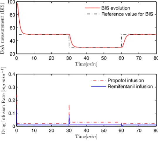
Figure 7 illustrates the performance of the control algorithm in the pres-ence of a change of the referpres-ence profile. In the first thirteen minutes it is intended that the BIS follows the reference 50, in the following thirteen

minutes the BIS reference level is set to 30 and in the last twenty minutes the BIS should again follow the reference level 50. It may be seen that the controller has a good performance also in this case. As expected, when the reference decreases there is a small bolus of propofol and remifentanil, in order to follow the reference, and when it increases no drug is administered.

0 10 20 30 40 50 60 70 80 20 40 60 80 100 Time[min] Do A m ea su re m en t (B IS ) BIS evolution Reference value for BIS

0 10 20 30 40 50 60 70 80 0 0.1 0.2 0.3 0.4 Time[min] Dr u g In fu si on R ate [mg mi n 1] Propofol infusion Remifentanil infusion

Figure 7: Evolution of DoA and of the dosages of propofol and of remifentanil, assuming changes in the reference profiles (zú_{= 50 from the beginning till t = 30 min, z}ú_{= 30 from}

t= 30 min till t = 60 min, and zú_{= 50 from then on), for ⁄ = 1, fl = 2.}

In a real clinical environment, the measurements of the patients BIS levels usually present a high level of noise, due to the nature of the sensors and the physiological ineheretic signs. This fact implies the existence of noise in the estimation of the states in the corresponding theoretical model. In Fig. (8) the evolution of the DoA of a patient is illustrated in the presence of noise in the measurement of the BIS level, that mimics the real data collected in the surgery room. For this purpose, a normal distribution N(µnoise, ‡noise),

where µnoise = 0 and ‡noise = 3 are respectively the mean and the standard

deviation, was used. As we can see, in spite of the presence of noise in the BIS measurements, the behavior of the controlled output of the patient is clinically accepted. 0 50 100 150 30 40 50 60 70 80 90 100 Time[min] D o A m ea su re m en t (B IS ) BIS evolution

Figure 8: Evolution of DoA in the presence of noise, for fl = 2 and ⁄ = 1.

5. A realistic simulation study

As a necessary preliminary step before implementation in clinical environ-ment, the performance of the controller proposed in this paper is tested on a bank of realistic simulated patients. These patients are simulated by means of PK/PD Wiener models (see Marsh et al. [19], and Minto et al. [20]) ob-tained from real data collected during eighteen breast surgeries. The patients (all female, with 54 ± 13 years of age, a height of 160 ± 5cm, and 69 ± 18Kg) were subject to general anesthesia under propofol and remifentanil adminis-tration. The DoA was monitored by the BIS and was manually controlled

around clinically accepted values by the anesthetist. Alaris GH pumps were used for both propofol and remifentanil. Infusion rates, BIS values and other physiological variables were acquired every five seconds (Mendon¸ca et al. [17]).

For each patient, the corresponding PK/PD Wiener model was obtained as follows. The parameters of the linear part were computed according to Marsh et al. [19], Minto et al. [20], and Schnider et al. [21] based on the rel-evant patient characteristics, whereas the parameters of the nonlinear part (generalized Hill equation) were identified from the surgery data, by Men-don¸ca et al. [17]. In order to test the proposed control strategy, each simu-lated patient is also modeled by the parsimonious parameter Wiener model of Silva et al. [10], with parameters identified as in Mendon¸ca et al. [17], and a control law of the form (37) tuned for that model is applied to the simulated patient. The set of parameter values identified by Mendon¸ca et al. [17] is given in appendix A, where also the corresponding relevant patient features that allow to compute the PK/PD model parameters are displayed. Here we present the results obtained for patients 9 and 15 of the database in two different simulations settings respectively. Patient 9 is a woman, with 51 years of age, a height of 163cm, and with 55kg. The corresponding identified parameters were: ECp

50 = 12.17, EC50r = 0.031, “ = 1.86, µ = 3.84,

– = 0.07, and ÷ = 0.28. Patient 15 is a woman, with 73 years of age, a

height of 160cm, a weight of 75kg, for which the identified parameters were:

EC₅₀p = 12.41, ECr

50 = 0.016, “ = 1.68, µ = 3.47, – = 0.10, and ÷ = 0.04.

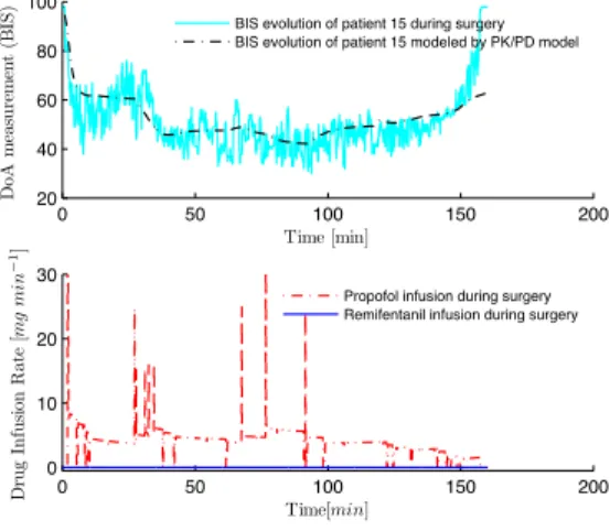
Figure 9 shows the BIS response of the patient 15 to the drug doses administered by the anesthetist during the surgery, along with the response

of the corresponding PK/PD model to the same drug input. The similarity between the two responses supports the idea of using the identified PK/PD models in order to simulate real patients.

0 50 100 150 200 20 40 60 80 100 Do A m ea su re m en t (B IS ) Time [min]

BIS evolution of patient 15 during surgery BIS evolution of patient 15 modeled by PK/PD model

0 50 100 150 200 0 10 20 30 Time[min] Dr u g In fu si on R ate [mg mi n 1]

Propofol infusion during surgery Remifentanil infusion during surgery

Figure 9: BIS response of the patient 15 (upper plot) to the drug doses administered by the anesthetist during the surgery (lower plot), along with the response of the corresponding PK/PD model to the same drug input. The average doses of propofol and of remifentanil reported were 4.21mg min≠1_{and 0.0147mg min}≠1_{respectively. Notice that propofol doses} above 30 mg min≠1_{are not represented in the graphic.}

In Fig. 10 the BIS response of the simulated patient 15 is presented, where the DoA control was performed using the control law (37) for tracking a BIS level of 50; this is an approximation value of the average real BIS obtained throughout the surgery. The selected proportion between the two drugs was the corresponding average reported in the monitored real case, fl = 286. The average of the doses of propofol and of remifentanil obtained by the controller were respectively 4.27mg min≠1and 0.0149mg min≠1; these values

respectively. The obtained set-point for the BIS level was 54.7, presenting an relative error of only 9%.

0 20 40 60 80 100 120 140 160 40 60 80 100 Time[min] Do A m ea su re m en t (B IS )

BIS evolution of the simulated patient 15

0 20 40 60 80 100 120 140 160 0 10 20 30 Time[min] Dr u g In fu si on R ate [mg mi n 1] Propofol infusion Remifentanil infusion

Figure 10: BIS response of the patient 15 and the infusion doses of propofol and of

remifen-tanil obtained by the proposed control law, for zú _{= 50, fl = 286, and ⁄ = 10. The}

average doses of propofol and of remifentanil obtained by the controller were respectively 4.27 mg min≠1 _{and 0.0149 mg min}≠1_{. Notice that propofol doses above 30 mg min}≠1 _are not represented in the graphic.

Figure 11 illustrates the application of the proposed control law to all the 18 simulated patients, for a desired reference BIS level of 50 (the remaining parameters are presented in the figure). As can be seen, the desired BIS level obtained in all the cases are very close to the desired one.

0 20 40 60 80 100 120 140 160 0 10 20 30 40 50 60 70 80 90 100 Do A m ea su re m en t (B IS ) Time [min]

BIS evolution of the 18 simulated patients

Figure 11: BIS response of all eighteen simulated patients (by means of a PK/PD model) controlled by the proposed control law, tuned for the corresponding parameter parsimo-nious model, for zú_{= 50, fl = 2, and ⁄ = 10.}

In Fig. 12 the performance of the control in the presence of a change of the reference profile and in the value of drugs proportion is illustrated (for patient 9). In the first ninety minutes it is intended that the BIS follows the reference 50, in the following thirty minutes the BIS reference level is set to 40 and in the last forty minutes the BIS is regulated to follow again the reference level 50. As expected, a reference decrease produces a peak in the doses of propofol and remifentanil, whereas when the reference increases no drug is administered. The proportion between the two drugs was fl = 0.2 in the first forty minutes and from then on it was changed to fl = 3. In spite of the variation of the drug proportion the BIS follows the desired reference. The possibility of changing the drug proportion during the surgery without affecting the reference tracking results constitutes a considerable advantage.

Indeed, clinical practice has often shown the need of adjusting the dosage profile according to the overall physiological response of the patient.

0 20 40 60 80 100 120 140 160 40 60 80 100 Time[min] Do A m ea su re m en t (B IS )

BIS evolution of the simulated patient 9

0 20 40 60 80 100 120 140 160 0 0.5 1 1.5 2 Time[min] Dr u g In fu si on R ate [mg mi n 1] Propofol infusion Remifentanil infusion

Figure 12: Evolution of DoA, of patient 9, and of the dosages of propofol and of

remifen-tanil, assuming changes in the reference profiles (zú_{= 50 from the beginning till t = 90min,}

zú_{= 40 from t = 90min till t = 120min, and z}ú_{= 50 from then on) and assuming changes} in the value of the drugs proportions (fl = 0.2 in the first forty minutes and from then on it was changed to fl = 3). ⁄ = 1.

6. Conclusion

A positive control law for multi-input positive systems was proposed in order to track a desired output reference value. This controller was applied in the control of the DoA, tracking the BIS level for a certain designed profile, by means of simultaneous administration of propofol and remifentanil, based on the parsimonious parameter model. This new Wiener model describes the joint effect of these two drugs and is adequate for model based control design since it presents a reduced number of parameters.

In this work it was theoretically proved that the controller may be tuned in order to achieve different convergence rates and different desired proportions between the dosages of these two drugs, in order to obtain a certain reference value for the BIS. Moreover, this controller also provides the possibility of changing the drugs proportion during the surgical anesthetic procedure with-out affecting the reference tracking results, which constitutes an interesting clinical advantage. Indeed anesthetic procedures during surgery relies on a defined DoA profile, but the change of the dosage profile due to the overall physiological response of the patient is often required.

The performance of the controller proposed in this paper was tested with success, by several simulations, on a bank of realistic simulated patients sim-ulated by means of PK/PD Wiener models obtained from real data collected. The simulation study illustrates the performance of the proposed controller under a variety of clinical conditions, like presence of noise measurement, changing of the doses proportions and of the reference profile.

References

[1] L. Farina, S. Rinaldi, Positive Linear Systems: Theory and Applica-tions., John Wiley & Sons, 2000.

[2] W. M. Haddad, T. Hayakawa, J. M. Bailey, International journal of adaptative control and signal processing (2003) 17: 209–235 (DOI: 10.1002/acs.737).

[3] B. Roszak, E. J. Davison, Proceedings of Workshop on Recent Advances in Control and Learning LNCIS 371 (2008) 181–193.

[4] B. Roszak, E. J. Davison, IEEE Transactions on Automatic Control 55(9) (Sept. 2010) 2204–2209.

[5] T. Kaczorek, Positive 1D and 2D systems, Springer, London, 2002. [6] J. C. Willems, Journal Automatica (Journal of IFAC) 12(5) (Sept. 1976)

519–523.

[7] K. Soltesz, G. A. Dumont, K. Heusden, T. H¨agglund, 51st IEEE Con-ference on Decision and Control (Dec. 2012).

[8] G. Bastin, A. Provost, in: Proceedings of the 15th International Sym-posium on Mathematical Theory of Networks and Systems (2002). [9] G. Dumont, Proceedings of the 8th IFAC Symposium on Biological and

Medical Systems (2012) (2012).

[10] M. M. Silva, T. Mendon¸ca, T. Wigren, Proceedings of the American Control Conference (ACC10) (2010) 4379– 4384.

[11] K. Godfrey, Compartmental Models and Their Application, Academic Press, 1983.

[12] J. P. LaSalle, The Stability of Dynamical Systems, SIAM, Bristol, Eng-land, 1976.

[13] R. I. Leine, N. Wouw, Stability and Convergence of Mechanical Systems with Unilateral Constraints, Springer-Verlag, German, 2008.

[14] X. Liao, L. Wang, P. Yu, Stability of Dynamical Systems, Elsevier, Netherlands, 2007.

[15] F. Bullo, Geometric Control of Mechanical Systems, Springer, USA, 2005.

[16] J. M. Bailey, W. M. Haddad, Control Systems Magazine, IEEE 25 (2005) 35 – 51.

[17] T. Mendon¸ca, H. Alonso, M. M. Silva, S. Esteves, M. Seabra, 16th IFAC Symposium on System Identification (2012).

[18] F. N. Nogueira, T. Mendon¸ca, P. Rocha, Proceedings of the 21st Mediterranean Conference on Control and Automation (MED’13) (2013).

[19] B. Marsh, N. Norton, G. N. Kenny, Br. J. Anaesthesia 67 (1991) 41 – 48.

[20] C. F. Minto, T. W. Schnider, T. D. Egan, E. Youngs, H. J. Lemmens, P. L. Gambus, V. Billard, J. F. Hoke, K. H. Moore, D. J. Hermann, K. T. Muir, J. W. Mandema, S. L. Shafer, Anesthesiology 86 (1997) 10 – 23.

[21] T. W. Schnider, C. F. Minto, P. L. Gambus, C. Andresen, D. B. Goodale, S. L. Shafer, E. J. Youngs, Anesthesiology 8 (1998) 1170 – 1182.

Appendix A. Database

This database was courteously provided by Galeno project (http://www2.fc.up.pt/galeno/). The parameters presented in Table A.2 were identified in Mendon¸ca et al.

Table A.1: Patient features

Gender Age Height (cm) Weight (kg)

Patient 1 F 56 160 88 Patient 2 F 48 158 52 Patient 3 F 51 165 55 Patient 4 F 56 160 65 Patient 5 F 64 146 60 Patient 6 F 59 159 110 Patient 7 F 29 163 59 Patient 8 F 45 155 58 Patient 9 F 51 163 55 Patient 10 F 32 172 56 Patient 11 F 68 160 64 Patient 12 F 50 161 68 Patient 13 F 68 158 113 Patient 14 F 70 161 78 Patient 15 F 73 160 75 Patient 16 F 34 162 57 Patient 17 F 43 155 62 Patient 18 F 66 155 74

Table A.2: PPM Parameters – ÷ “ µ Patient 1 0.0667 0.3989 2.0321 4.3266 Patient 2 0.0874 0.0670 1.0133 4.3845 Patient 3 0.0693 0.0482 2.0196 3.3133 Patient 4 0.0590 0.0425 1.8930 4.2273 Patient 5 0.0489 0.1269 1.0702 3.9505 Patient 6 0.0677 0.3373 2.6169 4.3774 Patient 7 0.0737 0.2793 3.7297 4.1494 Patient 8 0.0860 0.0212 0.9172 1.0000 Patient 9 0.0701 0.2837 1.8645 3.8367 Patient 10 0.1041 0.1038 1.4517 3.7978 Patient 11 0.0343 3.5768 0.9334 4.4496 Patient 12 0.0467 0.1254 1.6649 4.2860 Patient 13 0.0687 4.5413 0.9882 3.8094 Patient 14 0.0774 0.0397 3.8213 3.2302 Patient 15 0.0995 0.0377 1.6771 3.4726 Patient 16 0.0929 0.1205 3.9302 3.9983 Patient 17 0.0811 0.1033 1.6096 4.2064 Patient 18 0.1336 0.2307 1.5613 4.2411