CATÓLICA LISBON SCHOOL OF BUSINESS AND ECONOMICS
Mota-Engil – Equity Valuation
Sebastião Lima David Andrade Rocha
nº 152112058
July 2014
Dissertation submitted in partial fulfillment of requirements for the degree of MSc in Business Administration, at the Universidade Católica Portuguesa - July 2014
Abstract
Title: Mota-Engil – Equity Valuation
Author: Sebastião Lima David Andrade Rocha
The main goal of this dissertation was to reach the price per share of Mota-Engil Group as of the 31st of December 2013. In order to achieve such goal, in a first stage, we performed a Literature Review – gathering and presenting the most commonly used methods of equity valuation. Moreover, we concluded that the Discounting Cash Flow model (more specifically the Free Cash Flow to the Firm approach) was the most appropriate to value the price of Mota-Engil’s shares. Plus, we also show the results achieved through Relative Valuation. Our target price is 9.65€ per share whereas the price practiced by the market at such date was 4.32€. Thus, according to the model by us developed, Mota-Engil’s shares were undervalued, in the end of 2013.
Acknowledgements
For the precious help and availability, I would like to thank Dr. João Vermelho (Mota-Engil Investor Relations) and of course Prof. José Tudela Martins for all the guidance.
Finally, I want to dedicate this dissertation to my family and Rita who have always been there for me.
Nomenclature:
APV: Adjusted Present Value CF: Cash Flow
FCFE: Free Cash Flow to Equity Ke: Cost of equity
Rev: Revenues
Op. expenses: Operating expenses D&A: Depreciation and Amortization Int.: Interest
Pref. Div.: Preferred Dividends CAPEX: Capital Expenditure W.C.N: Working Capital Needs Princ.: Principal repayments
New debt: Proceeds from issuing new debt CAPM: Capital Asset Pricing Model
Rf: Risk-free Rate
E: Equity beta (Systematic risk of investing in a specific security, compared to the market it
is inserted in)
E(Rm): Expected return of market portfolio
E(Rm)- Rf: Market Risk Premium
FCFF: Free Cash Flow to the Firm DCF: Discounted Cash Flows
EBIT(1-t): Earnings before interest and taxes, after taxes
EBITDA: Earnings before interest, taxes and depreciation and amortization Kd: Cost of debt
CCF: Capital Cash Flows VL: Value of levered Firm
VU: Value of unlevered Firm
PV: Present Value g: Growth rate
KeU: cost of equity unlevered
EVA: Economic Value Added
(also called NOPLAT): Net operating profit after taxes;
Dbv: Debt Book Value;
Ebv: Equity Book Value;
P/E or PER: Price to Earnings Ratio PBV: Price to Book Ratio
EV/Sales: Enterprise Value to Sales Value Ratio EV/Sales: Enterprise Value to EBITDA Value Ratio ROIC: Return on Invested Capital
Table of Contents
I. Introduction ... 1
II. Literature Review ... 2
II.1. Discounted Cash Flow Valuation ... 3
II.1.1. Free Cash Flow to Equity and Cost of Equity ... 3
II.1.2. Free Cash Flow to the Firm and Cost of Capital... 5
II.1.3 Capital Cash-Flow and WACC before taxes ... 8
II.1.4 Adjusted Present Value ... 9
II.2. Value Creation Valuation Models ... 12
II.2.1 EVA ... 12
II.2.2 Economic Profit... 13
II.3. Relative Valuation ... 14
II.3.1 P/E Ratio or PER ... 15
II.3.2 Price to Book ... 16
II.3.3 EV/Sales ... 16
II.3.4 EV/EBITDA ... 17
II.4. Contingent Claim Valuation ... 18
II.5. Summary ... 19
III. Company Presentation ... 20
III.1. Overall Performance ... 22
III.2. Performance in Stock Market: ... 25
III.3. Europe... 26
III.3.1. Portugal ... 26
III.3.2. Poland ... 27
III.4. Africa ... 28
III.5. Latin America ... 29
IV. Company Valuation ... 30
IV.1. Discounted Cash Flow Valuation: Free Cash Flow to the Firm ... 30
IV.1.1 Sales & services rendered ... 31
IV.1.2 Gross Profit ... 33
IV.1.3 EBITDA ... 34
IV.1.4 EBIT ... 36
IV.1.5 Capital Expenditure (CAPEX) ... 38
IV.1.6 Depreciation and Amortization ... 39
IV.1.7 Change in Working Capital ... 40
IV.1.8 Tax rate ... 41
IV.1.10 Risk-free Rate ... 41
IV.1.11 Beta ... 41
IV.1.12 Country-Risk Premium and Market-Risk Premium ... 42
IV.1.13 Cost of Equity ... 42
IV.1.14 Cost of Debt ... 42
IV.1.15 Leverage ... 43
IV.1.16 Weighted Average Cost of Capital ... 44
IV.1.17 Growth in Perpetuity ... 44
IV.1.18 Terminal Value ... 45
IV.1.19 Enterprise Value ... 45
IV.1.20 Minority Interests ... 45
IV.1.21 Martifer, Ascendi, Indaqua and Financial Investments ... 46
IV.1.22 Price per Share ... 47
IV.2. Relative Valuation ... 48
IV.2.1. Peer Group Definition ... 48
IV.2.2. Multiples ... 50
V. Investment Bank results - Comparison ... 51
VI. Sensitivity Analysis ... 54
VII. References ... 56
I. Introduction
Valuation is the action of estimating the value of something. We, as human beings, have developed this need for attributing an analytical value to almost everything. It is the value that we perceive that guides us in our routine in all kinds of trading and investing activities, among others.
Many people around the world use valuation for numerous purposes. Starting with students like me who decide to embrace this task of reaching a value for a company’s equity, through financial analysts and ending in investors.
In this dissertation, valuation comes up more as a financial and quantitative measure regarding the estimated value of the shares of a company. However, valuation, in these specific terms, can provide us the value of the Equity but also the value of the whole Firm. The main purpose of this dissertation is to reach the target price for Mota-Engil shares. Firstly, we start by presenting the literature developed on Valuation Models. The goal here is to provide the reader with a contextualization on the common practices and the most broadly used and accepted methods for valuing companies.
Moreover, we explain the specificities of each model including the advantages, disadvantages and the applicability (or not) to a company with Mota-Engil’s characteristics. Taking all those into consideration, we choose the valuation model(s) to use throughout the rest of the dissertation.
Furthermore, we write a chapter introducing the company to reader. We provide an historical background of Mota-Engil, including the main historical facts from the creation of Mota & Companhia to the merger of Mota & Companhia with Engil, passing through the important steps by those two companies both separate and merged.
Additionally, we show how the group is organized nowadays and describe the sectors and regions in which it operates.
Following the choice of our model(s) and the company presentation, we provide our valuation of Mota-Engil. In this part, we explain our assumptions, methodology and results achieved.
After having a target price, we test its coherence by comparing it with an Investment Research by Caixa BI, the Investment Bank of Caixa Geral de Depósitos Group, which contains an equity valuation of Mota-Engil.
II. Literature Review
There are many models and techniques to reach the value of a firm and its corresponding equity. Those have been developed over the years and hopefully will continue that way in the future.
Every model has limitations and advantages when compared to others and all they provide is an approximation to the real value of a firm, since it is very hard (if not impossible) to identify all the factors influencing the value of a firm and also to attribute an accurate numerical value to the factors taken into account.
In this chapter, we present some of the existing valuation methods, showing each method’s advantages and disadvantages.
First of all, let us state and briefly explain the most used methods to reach both equity and firm values.
According to Damodaran (1994), the approaches to valuation may be divided in three broad groups: Discounted Cash Flow Valuation, Relative Valuation and Contingent Claim Valuation.
We will complement Damodaran’s division and add another “category” proposed by Fernandez (2013a), related to Value Creation.
Further, we will describe four Discounted Cash Flow Valuation models suggested by Fernandez (2013a): Equity cash flow, Free cash flow, Capital cash flow and APV.
As for Value Creation Valuation Models, we provide a review of two models: Economic Value Added and Economic profit.
Inside Relative Valuation subchapter we include a perspective about the use of multiples (describing the ones most widely used) and a literature review regarding the definition of a Peer Group.
Finally, we describe the main topics regarding Contingent Claim Valuation.
At last, we will summarize the main conclusions taken from this literature review chapter that will be helpful for the rest of our work.
II.1. Discounted Cash Flow Valuation
For the Discounted Cash Flow Valuation, the basic discounting principle is used. The elements needed are cash flows and a discount rate, at which those cash flows are discounted. Basically, the following formula summarizes it:
∑
However, several approaches, inside the Discounted Cash Flow Valuation model, have been developed.
The value arising from each of these methods brings the same result for all the others, if the same assumptions are used. What changes among them is the basis cash-flow and discounting rate considered.
Taking this into consideration, we present those four models, previously mentioned and then choose the most appropriate to use in our valuation, considering company’s characteristics and availability of accurate data regarding the inputs needed.
II.1.1. Free Cash Flow to Equity and Cost of Equity
Let us start with the Free Cash Flow to Equity (FCFE from here on) that is discounted at the required return to equity or cost of equity (Ke from here onwards).
∑
First of all, FCFE is, in very simple terms, the “money (cash) that goes from the Cash of the company to the pockets of shareholders.”1. In other words, FCFE “is, therefore, the cash
flow after operating expenses, interest and principal payments, and any capital expenditure needed to maintain the growth rate in projected cash flows.”2. The way in which the FCFE is
computed depends on whether the firm is levered or not, i.e. if it includes debt in its capital structure or not. 1 Fernandez (2013b) 2 Damodaran (1994)
Below we present the components and corresponding computations to reach FCFE for a levered firm3:
For an unlevered firm, we disregard cash-flows related to debt (as previously stated), so in the previous formula we would not consider Interest expense, Principal repayments and Proceeds from new debt issued.
When using the FCFE approach to reach the value of a firm, we will need to compute the cost of equity as it represents the appropriate discounting rate, as it is possible to understand by its definition.
Regarding Ke, we can say that it represents “the rate of return that investors require to make
an equity investment in a firm”4
. To calculate such discount rate, Damodaran suggests two ways. The first one is to use Capital Asset Pricing Model (CAPM from here on) and the other is through the use of a dividend growth model. We will use CAPM to calculate our discounting rates as it is broadly acknowledged.
CAPM is a model which relates expected return with risk. Basically, according to this model, an investor of a firm must be compensated somehow due to two factors.
The first one is the time value of money – coming from one of the assumptions of this model, which assumes that everyone can lend and borrow at the risk-free rate (Rf from here on) -,
i.e. an investor must receive at least the amount that he would receive if he had put his/her money in a deposit.
The other compensation is related to the additional risk that the investor is taking by investing in that specific firm.
According to this model, the cost of equity may be obtained through the following formula:
Another element that can and will be introduced throughout our work is the Country Risk Premium. This element refers to the additional premium required by investors because of all
3
Damodaran (1994) 4
the conditions lived in each country (political, geographical, etc.) that influence investors’ decisions. So, our final formula to compute the cost of equity is:
[ ]
By discounting FCFE to for every period we are considering, we reach the value of the equity of the firm.
II.1.2. Free Cash Flow to the Firm and Cost of Capital
The most commonly used Discounting Cash Flow model is the Free Cash Flow to the Firm (FCFF from now on), discounted at the Weighted Average Cost of Capital (WACC). The formula may be presented as follows:
∑
The basic difference between these two varieties of the DCF model is that the FCFE does not include cash flows related with debt. By discounting the FCFF, the enterprise value is obtained referring to the assets of all claimholders (both equity and debt holders), while through discounting FCFE the value obtained corresponds to the value for the owners of stock or preferred stock (or any other kind of equity instrument).
It is important to note that Earnings before interest and taxes are computed after taxes because taxes on earnings are not free cash flows to the firm.
Moreover, by using EBIT instead of EBITDA we consider the value of earnings with Depreciation and Amortization to reach the value of earnings after tax because Depreciation represents a cost that decreases taxable income for the company and is, thus, included in taxation. Afterwards we add back Depreciation and Amortization, because it does not represent a cash outflow;
Regarding the discount rate, we have already stated above that we use WACC to discount the FCFF values.
Weighted Average Cost of Capital is the weighted average of the cost of all funding source of a firm, i.e. debt, equity and other. In our case, and disregarding other funding sources as it
is not applicable to Mota-Engil, the formula for reaching the Weighted Average Cost of Capital is the one proposed by Damodaran (1994):
Let us explain the components of the formula above (excluding cost of equity, previously described and explained). The cost of debt- - represents the cost that the firm has to incur in to get funding from external sources. The value used is deducted from taxes because interest expenses are tax deductible and hence decrease the cost of debt of the firm. Damodaran suggests three components to take into consideration when estimating the cost of debt: 1- Current interest rates; 2- Company’s default risk and 3- Tax advantages associated. To value Debt at market values we chose to use Damodaran’s5 suggestion:
(
) Moreover, we also use the value of Equity and Debt. Regarding these two, there is an interesting question regarding the choice of market or book values. There are different opinions.
On one hand, it is said that on a conservative basis it is more appropriate to use book values as those are less volatile (enhancing reliability). Furthermore, it is argued that “lenders will not lend on the basis of market value”6.
On the other hand, Damoradan refutes all the reasons favoring the use of book values, stating that those are more based on perception than on real facts and that the “true value of the firm changes over time as both firm-specific and marketwide information is revealed.”7.
So, Damodaran defends that the values to use in these cases are the market ones because “the cost of capital measures the cost of issuing securities, stocks as well as bonds, to finance projects and that these securities are issued at market value, not at book value.”8.
Similarly, Copeland et al (1994) write: “The first step in developing an estimate of the WACC is to determine a capital structure for the company you are valuing. This provides the market
5 http://pages.stern.nyu.edu/~%20adamodar/New_Home_Page/valquestions/mktvalofdebt.htm 6 Damodaran (1994) 7 Damodaran (1994) 8 Damodaran (1994)
value weights for the WACC formula (…) The best approach for estimating the market-value based capital structure is to identify the values of the capital structure element directly from their prices in the market place”.9
Hence, during our work we will use market values for determining the current market values capital structure and use it as a target for the remaining years.
Furthermore, the FCFF model may have many other variants. It may vary according to the growth pattern of the firm. If the firm has a steady-state growth, then a year might be enough to reach its firm/equity value.
However, if the firm is cyclical or is not in a steady-state growth, a more extended period must be taken into account in order to reach a consistent value. In these cases, there are the two-stage or even three-stage approaches. These relate to the number of stages that need to be considered for the company to be in an equilibrium situation.
Our analysis relies on a two-stage growth model as we consider a first period that corresponds to the company’s path to reaching a steady growth in perpetuity (second and final stage). So, in this case:
∑ With:
This DCF approach is one of the most commonly accepted (if not the most).
Its main advantages are the easiness to use since it only requires a small set of information and the fact that it “captures all the elements that affect the value of a company”10.
Moreover, the DCF approach is very adequate for multi business companies as it is able to put together the different cash flows from different businesses, discounting them at separate rates (representing the risk of each separate business).
Plus, this valuation model is not as influenced by market errors as others, since the majority of information needed is firm-specific.
9
Copeland et al. (1994) 10
However, there are several situations in which problems may arise by using the DCF model. As referred by Damodaran, firms in trouble, cyclical firms, firms with unutilized assets, firms with patents or product options, firms in the process of restructuring or involved in an acquisition process and private firms may be very hard to valuate through DCF approach, since the period, the discounting rates and the expected cash flows are much harder to reach as the level of uncertainty and lack of available data increases.
II.1.3 Capital Cash-Flow and WACC before taxes
Capital Cash Flow (CCF) corresponds to “the sum of the debt cash flow plus the equity cash flow (…) It is important to not confuse the capital cash flow with the free cash flow”11.
This model discounts CCF at WACC before taxes to reach the value of the firm:
∑
According to that same paper, Fernandez writes the formula to compute CCF:
WACC before taxes follows a computation similar to one previously provided. The only difference is the fact that taxes are not considered. Hence:
Moreover, a characteristic of this model is that “is easier to apply whenever debt is forecasted in levels instead of a percentage of total enterprise value”12.
This model will not be considered in our valuation as it is not as widely used as others and because, as it is written above, it works better in cases where debt amounts can be forecasted in absolute terms, which is not the case of the debt level of Mota-Engil.
11
Fernandez (2013a) 12
II.1.4 Adjusted Present Value
The Adjusted Present Value model (APV) is similar to the other Discounted Cash Flow valuation models. The distinctive feature of this model is the fact that the company is valued by its operating assets (as if the firm was unlevered) by discounting the FCFF to a certain discounting rate, in a first stage, and then through the net effect of benefits (taxes) and costs of having debt in its capital structure. There are many theories and ways of computing the elements included in the model.
In order to better understand the model, let us provide you with an historical literature review on this model.
It all started with Modigliani and Miller (1958), when those two gave emphasis to the impacts of the capital structure in the value of firms. However, in this first study13 they argued that there was no relevance on such impacts as they assumed a society with no taxes.
This was definitely the beginning of a series of studies and investigations on this subject but there were several assumptions that made this model sill not very applicable in real life: it assumed perfect capital market conditions (no transactions costs, no taxes, straight prices, no asymmetry of information, no barriers to entry and access to same interest rates by every player in the market).
The conclusion of this first study was that the value of a levered firm would be the same as an equal one funded with debt:
Moreover, five years later, those same two authors reviewed their opinion in Modigliani and Miller (1963)14 where this matter of the value of interest tax shields and the impacts of leverage in the capital structure of a company was first and importantly developed.
The authors realized that a company funded only with equity would not be able to deduct taxes (dividend payments do not reduce tax) as the firms that used debt to fund the company. Part of the interest expense on debt would not be considered for tax calculation, creating this incentive to fund the company not only with equity but also with debt.
Taking this into account, they concluded that a company with debt against an unlevered firm, ceteris paribus, should have a higher value and that the difference in value corresponded exactly to the tax savings above described
13
Modigliani and Miller (1958) 14
In this book, the authors proposed that the interest tax shields should be valued by discounting the value of tax savings related to interest on risk-free debt at the risk-free rate (RF):
So, now we had the following computation for the value of a firm:
The model was now more accurate, but there was still room for improvement.
Myers (1974) points out that the interest expense should not be computed with the risk-free rate, as firms and investors do not have access to the same interest rate on debt. Consequently, each player in the market has different interest rates that pose more risk than risk-free assets, represented by Kd – cost of debt.
Therefore, it is concluded that the present value of interest tax shields should be computed as follows:
Further, in Miller (1977), it is argued that there is “the other side of the coin” regarding interest tax shields. We have seen in the previous paragraphs that there was an incentive for firms to contract debt because they would be able to reach a higher value for the firm by saving in taxation.
Miller introduces the bankruptcy and distress costs that arise from contracting debt and the impact of individual taxation. He concludes that “even in a world in which interest payments are fully deductible in computing corporate income taxes, the value of the firm, in equilibrium will still be independent”15.
Let us now present Damodaran16 suggestion regarding APV, as it includes the several aspects we have been introducing in the previous paragraphs about this model:
15 Miller (1977) 16 http://pages.stern.nyu.edu/~adamodar/New_Home_Page/valquestions/apv.htm
The value of the unlevered firm is reached by discounting FCFF at the unlevered cost of equity (computed with the unlevered beta instead of the usual –levered- one):
Tax benefits from borrowing, if viewed as perpetual are computed:
Finally, the present value of expected bankruptcy corresponds to the product of the expected bankruptcy costs by the estimated probability of bankruptcy occurring:
This model is considered by many as more accurate in terms of splitting the components clearly and evaluating its impacts on the firm’s value.
However, in practical terms there are many mistakes that may arise from using this model such as the possibility of ignoring or badly estimating expected bankruptcy cost. This will cause firm value to be overestimated.
II.2. Value Creation Valuation Models
Value creation valuation models or residual income provide the same results as the Discounted Cash Flow models. This becomes obvious “since all the methods analyse the same reality under the same hypothesis”17.
The major difference between these models is that the components of these models are not cash-flows and “their financial meaning is much less clear than that of cash-flows”18.
Below we describe the following models: EVA (Economic Value Added), Economic Profit. We will not put as much emphasis in these models as in the previous ones as they are not so commonly used to value companies. These methods will not be considered for our valuation.
II.2.1 EVA
Economic Value Added refers to the surplus obtained in a certain investment. Using this to the totality of projects of a company as well as the assets in place, the value of the firm can be obtained.
Damodaran19 writes that:
According to Pablo Fernandez20, we can obtain EVA in the following formula:
Combining the two formulas, by applying EVA to the projects and assets in place, the value of the firm can be reached.
17 Fernandez (2013c) 18 Fernandez (2013c) 19 http://pages.stern.nyu.edu/~%20adamodar/New_Home_Page/lectures/eva.html 20 Fernandez (2013c)
II.2.2 Economic Profit
Fernandez states that economic profit is “book profit less the equity’s book value multiplied by the required return on equity”21.
For reaching the firm value through Economic Profit, we sum present value of economic profit for each period (discounted at the cost of Equity) to the previous year Equity value. The following formula is suggested:
∑
21
II.3. Relative Valuation
The Relative Valuation approach consists on reaching the value of an asset (or firm) by using information on similar/comparable assets.
Applying this approach to Equity Valuation, the method consists on using the market value of similar firms, through the use of multiples, in order to obtain a value to the firm being valued. The first step to this approach is to define a peer group, i.e. a group of companies that share many/some characteristics with the company we want to value. After having the group of comparable firms defined, the market value of such firms must be obtained.
In order to be able to compare the market values obtained we need to standardize them, as most of the times the values are not similar in absolute terms. From this standardization, common variables arise and they may relate to earnings, revenues, book value and many other indicators. These common variables represent the usually called multiples.
Finally, through the use of multiples and by applying them to the earnings/revenues/book value of the company, we reach a possible value for the equity of the firm.
Multiples may be divided in two broad groups: Equity-based multiples and Enterprise Value-based multiples.
The difference is simple: the first group uses the value of Equity as a reference, while the other uses the Enterprise Value.
Some of the most commonly used Equity-based ratios are the price/earnings ratio (P/E) and price/book value ratio (PBV). Regarding the second group the most widely used are: EV/Sales ratio and EV/EBITDA.
Regarding the usage of multiples, they have a tremendous advantage which is the fact that they can simply and quickly provide a value for firms.
However, there is a set of disadvantages regarding this approach.
First of all, the definition of the peer group is always subjective to inaccuracy since two firms are never equal. Plus, a peer group is normally a set of companies that comprises more than two firms, so the differences and inaccuracies are multiplied.
Moreover, not only the companies have differences, which biases the valuation from the beginning, but also the values attributed to each comparable firm, by the market, may contain errors itself (even if on average the market tends to price assets correctly), i.e. both
the choice of comparables and the fact that they may be under/overvalued will always have a “hidden” impact on our usage of relative valuation.
Let us now refer to what previous studies on this matter show.
According to Fernandez (2013d), “multiples almost always show a broad dispersion which is why valuations performed using multiples are highly debatable”. This leaves us with a notion that our relative valuation may not be as accurate as other possible methods. Nevertheless, that same author emphasizes the importance of multiples as a point of evaluation for when other methods are used.
Goedhart et al. (2005) suggest some basic principles to fulfill when working with multiples on valuation. First, it is suggested that ROIC and growth projections should be the key criteria to define a group of comparables. According to Damodaran (1994), choosing comparables based on industry can be quite misleading because even if firms are defined as of belonging to the same industry, they may be subject to an enormous variety of risk and have very different growth profiles.
Secondly, it is advised to use forward-looking multiples rather than those based on historical results. Moreover, the use of Enterprise-value multiples is also suggested.
Below, we describe the most widely used and recommended multiples:
II.3.1 P/E Ratio or PER
Price to Earnings Ratio relates the price of the share of a company with the earnings. Its intuition is quite simple (as the one for most multiples) and this is probably the most “popular” multiple used for valuation purposes. Summarizing, the multiple is as follows:
This ratio may also be seen without a per share quantity, using the total Market Capitalization and Net Income, instead of the values presented in the formula.
There is another reason why PER is so widely used, other than simplicity. According to Damodaran (1994), PER is proxy for several important characteristics of firms such as growth and risk. However, Damodaran also mentions some problems when using PER. First
of all, this multiple does not work in a case where the firm has negative earnings. Thus, for cyclical firms this multiple cannot be used with reference to all periods.
II.3.2 Price to Book
Price to Book ratio provides a reliable measure for the value of the firm. Again, the multiple is simple:
Damodaran (1994) states that book values provide a stable measure of each company that can be easily compared to the market value of that same firm, as it is a very simple benchmark. Another advantage that is also mentioned is that accounting standards are quite consistent which allows having a good comparison between different companies. However, that turns out to be also a disadvantage as any change in the accounting policies may lead to very misleading results.
Compared to PER, this multiple has the advantage of being able to work even if earnings are negative. Nevertheless, there are firm such as services firms in which the accounting values are far from representing the companies’ true value.
Finally, if a firm has “a sustained string of negative earnings reports” 22the price to book ratio
becomes negative.
II.3.3 EV/Sales
Once again, the concept that supports this multiple is quite simple:
One of the main advantages of this multiple is that it can never be negative. This is clearly an advantage if compared to the previous two multiples.
Furthermore, as referred by Damodaran (1994) unlike the previous multiples accounting policies and other changes can hardly manipulate revenues and sales, meaning that it is quite a reliable source.
22
Nonetheless, there is another element that decreases the reliability of this multiple because sales may not change much even if profitability decreases a lot, since revenues and sales do not determine the success and value of a firm.
II.3.4 EV/EBITDA
“This multiple is one of the most widely used by analysts”23.
The formula in this multiple, again, comes for the way it is called:
According to Fernandez24 there are two big flaws of this multiple: 1- It does not consider working capital requirements. 2- It excludes capital investments.
Further, Moody’s (2000) presents other critical fails of using EBITDA in these multiples. One of them is that EBITDA is not the same under different accounting standards; secondly EBITDA does not portray the quality of earnings.
Still, it is one of the most widely used because of its availability and we will be using it in our relative valuation. 23 Fernandez (2013d) 24 Fernandez (2013d)
II.4. Contingent Claim Valuation
Damodaran (1994) defines Contingent Claim “or option as an asset that pays off only under certain contingencies”. These methods of valuation assume that assets have similar characteristics to options. Of course, they are only effective in securities that share some characteristics of options such as: defined fixed life and dependence from an underlying asset.
Fernandez25 suggests approaches like the Black Scholes model and Investment Option model.
Damodaran points out some of the advantages and disadvantages of using contingent claim valuation:26 The main advantage is that these option models are very helpful in cases where no other method is effective.
Nevertheless, the disadvantages are the fact that inputs are sometimes very hard to obtain, it requires assets to be valued (“It is therefore an approach that is addendum to another valuation approach”27) since it does not give the value of the firm but the value of one or
some assets. Consequently, the last disadvantage leads to another disadvantage that relates to the possibility of double counting.
We will disregard this type of valuation because Mota-Engil does no really have any asset that has the option characteristics above described.
25 Fernandez (2013a) 26 http://people.stern.nyu.edu/adamodar/pdfiles/eqnotes/ValIntro.pdf 27 http://people.stern.nyu.edu/adamodar/pdfiles/eqnotes/ValIntro.pdf
II.5. Summary
After presenting different kinds of valuation models, we now choose those that we will use to value Mota-Engil’s share. Throughout this chapter we pointed out each method’s advantages and disadvantages. Let us now formalize the models to use in our valuation. First of all, we will use the Free Cash Flow to the Firm (FCFF) as our main valuation model. The reasons for this choice are presented in the subchapter of this model. In our opinion, the trade-off, among all the models, in terms of simplicity, data availability, applicability to Mota-Engil’s characteristics and effectiveness tells us that FCFF is the most appropriate model to value Mota-Engil.
Additionally, we will complement our FCFF valuation with a Relative Valuation. The values obtained (through P/E, Price to Book, EV/EBITDA and EV/Sales multiples) will serve as an indicator and matter of comparability for our main model, following authors’ suggestions regarding the importance of relative valuation.
III. Company Presentation
Mota-Engil is a Portuguese Group considered one of the 30th largest groups in the construction area in Europe.
Let us first provide you with the historical background of this group. It is important to refer that all the information below was provided by the Investor Relations Department, Mota-Engil institutional presentation28, Group’s website and 2012 and 2013 Annual Reports.
In 1946, more precisely on the 29th of June, Manuel António da Mota founded Mota & Companhia, in Amarante. A few weeks after the foundation of Mota & Companhia, a branch office was created in Angola. Until 1974, the company only operated in Angola. At first, the core business was related to the transformation of wood and only afterwards, around 1948, the company focused on the construction sector, mainly in public works.
The first big public work performed by Mota & Companhia was the International Airport of Luanda and it was the beginning of a successful path in the construction sector.
In 1954, the company Engil is renewed with the entrance of António Valadas Fernandes. Already inserted in the construction sector in Lisbon, in 1961, Engil gains its first contract outside Lisbon for the construction of a school in Castelo Branco.
Some years later, around 1975, Mota & Companhia started its internationalization and started projects in Namibia and Swaziland.
In the following year, Mota & Companhia started to operate in Portugal on the construction of a dam. This led the company to win huge public work projects and later becoming the third largest company in the country.
In 1987, Mota & Companhia, previously a limited company, became a joint-stock company and after a subsequent capital dispersion requested its presence in the stock market.
Engil, in 1987, became a group with participations in other firms and acquired several companies in the following years. This happened to face the evolution of demand and the need of diversification.
Consequently, Engil began the internationalization process (1989), starting in Angola, then Mozambique, Germany and Peru.
28
Mota & Companhia also opted to diversify its activities, entering in several markets including ceramics products, vehicles, real estate, sea transportation and road signs. In 1994, the consortium that included Mota & Companhia won the contest to build Vasco da Gama Bridge, which was a huge event in the history of the firm.
On the 23rd of July 1999, Mota launched a proposal to acquire all the shares of Engil and, already in 2000, the operation was concluded and Mota-Engil was born similar to how we know it today. With this merger, Mota-Engil was now the largest construction firm in Portugal.
At the same time, the new group was determined to diversify, especially in areas like transportation concession and Environment and Services. After several adjustments following the merger were made, the group defined its four independent business areas: Mota-Engil Engineering and Construction, Mota-Engil Environment and Services, Mota-Engil Concessions and Transports and Mota-Engil Housing and Tourism.
In 2004, there is reinforcement in the international backlog in Eastern Europe leading to the creation of Mota-Engil Polska, the fourth largest construction firm in Poland.
In the following year (2005), Mota-Engil enters PSI20, the Portuguese Stock Index after leading the candidates’ list for several months. This event obviously led to an even higher visibility of the Group.
After introducing the history of the Group, let us now describe how the Group is organized nowadays.
For the Engineering and Construction business, Mota-Engil operates in infrastructures, building, real estate and other specific projects. Concerning the Environments & Services sector, Mota-Engil’s projects includes waste management, ports and logistics, water management, energy and multiservice. Regarding Concession and Transports sector, it includes services related to Highways, Bridges, Railways and Subway. Finally, there is the Mining business where Mota-Engil covers Prospecting, Extraction and Exploitation activities. Mota-Engil Group is the leader in the construction, port operations and waste management sectors in Portugal. Moreover, the group presently owns participations in more than 200 companies and is present in 3 continents including 20 countries.
Up until 2011, the Group’s structure was organized by business area. However, starting in 2012, the Group decided to organize itself by geographies: Europe, Africa and Latin America.
III.1. Overall Performance
Let us now present the evolution of some financial indicators in previous years (2007-2013). The goal is to allow the reader to have an even better understanding on ME’s situation. Turnover:
Regarding turnover, we may say that ME has been able to continuously increase turnover despite the financial crisis. During this period, ME has always had a higher sales level than in the previous year.
Chart 1 – Turnover evolution (2007 to 2013). Source: Annual Reports
As previously stated, ME changed the structure of the Group, in 2012, and decided to organize itself by region. Thus, ME only provides data by region starting in 2011.
Chart 2 – Turnover by Business Area. Source: Annual Report 2013 0 500 1,000 1,500 2,000 2,500 3,000 2007 2008 2009 2010 2011 2012 2013 T u rn o v er L ev el (M illi o n E u ro s) Turnover Linear (Turnover)
From Chart 2, we can see that, in 2013, Africa has reached a similar sales level to the one in Europe. Plus, we can also observe that Latin America plays already an important role in terms of turnover for the Group. Hence, the projections are that Africa and Latin America will have higher sales than Europe in medium/long-term, as we show ahead in our work.
Backlog:
Following the trend of turnover, total backlog has been increasing and there have been changes regarding the weight of each regions value on total backlog. Again, we only had access to information on backlog by region for 2012 and 2013.
Chart 3 – Backlog distribution by region
Moreover, despite the changes on the distribution of total backlog by region, this total value has developed as follows:
Chart 4 – Backlog evolution (in million euros)
30% 23% 44% 42% 26% 35% 0% 20% 40% 60% 80% 100% 2012 2013 Latin America Africa Europe 0 500 1,000 1,500 2,000 2,500 3,000 3,500 4,000 4,500 2007 2008 2009 2010 2011 2012 2013
Capital Structure
ME has had a constant leverage ratio. The main Group’s activity (Engineering & Construction) requires a lot of investment and these firms are able to contract higher amounts of debt as they have many assets that may pose as collateral to the banks. Plus, ME’s reputation in the market also allows for banks to fund the Group. There are many different opinions regarding the optimal debt level for each firm. However, there is no consensus and we have no receipt or fixed value for the optimal leverage ratio.
Chart 5 – Capital Structure from 2007 to 2013
Nonetheless, the fact that debt has been representing around 80% of total capital leads us to conclude that ME leverage ratio is quite high.
0% 10% 20% 30% 40% 50% 60% 70% 80% 90% 100% 2007 2008 2009 2010 2011 2012 2013 E/V D/V
III.2. Performance in Stock Market:
Let us now give you a better perspective on how Mota-Engil’s shares have been trading in the stock market (PSI 20 Index). We believe that a chart is the best way to provide such perspective:
Chart 6 – Mota-Engil price per share in the last five years
From 2008 to 2013, it is possible to see a huge increase in the price of Mota Engil’s shares (from 2.35€ on the 31st of December 2008 to 4.32€ on the 31st of December 2013).
Moreover, we can observe that the price evolution was far from linear, having a downwards trend from 2009 and 2011.
However, the price per share does not, by itself, show the performance of the stock. Taking that into account, we chose to compute the total shareholder return. For an investor that invested in Mota Engil on the 31st of December of 2008 we reached the following results:
Years Considered 5 Dividends (constant) 0.11 Price 31st December 2008 2.35 Price ex-div 12/05/2009 3.29 Price 31st December 2013 4.32 Capital Gain 31.3% Dividend Gain 16.7%
Total Shareholder Return 48.0%
Box 1 – Total Shareholder Return 0 0.5 1 1.5 2 2.5 3 3.5 4 4.5 5 P ric e per s har e ( €)
III.3. Europe
Mota-Engil operates in seven countries in Europe: Portugal, Spain, Ireland, Poland, Czech Republic, Slovakia and Hungary. During the year of 2013, there was a backlog of 905 million Euros; total turnover of 911 million Euros which generated an EBITDA level around 85.5 million Euros.
III.3.1. Portugal Engineering & Construction
ME activities in Portugal have been suffering a lot with the financial crisis that affects Portugal and many countries in the world. This crisis led to a decrease in demand (as there are less construction projects) and backlog is being consumed at a fast rate. Since public work construction projects, the core business of the Group, have been quite stationary the firm has been investing in buildings (e.g. the construction of Zon Headquarters and EDP Headquarters and dams).
ME was able to somehow predict the financial crisis reallocating equipment and personnel to the emerging market it operates in (Africa and Latin America). This allowed having a huge cost reduction in the most affected geographies.
Environment & Services
In an attempt to diversify, ME invested in Suma Group (controlling around 61.5%). Suma is market leader in waste management. There has been a decrease in earnings associated with this activity. The main reason is the fact that remuneration is made by volume and with the crisis there was slightly less consumption and consequently less waste to manage. Further, there has also been a reduction in prices. These contracts are valid for 5 to 7 years and every time they are renewed, prices go down since less Capital Expenditure is needed. Another activity in the diversification by ME is Port Concessions. For that purpose, ME acquired Tertir becoming market leader in Containers Management sector. This leadership includes having concessions in all main ports in Portugal, except for one (Sines Port).
This Port Concession segment is the one growing the most in Portugal, considering all ME’s activities.
Moreover, ME, as stated above, also operates in Water Management segment, as it has 6 concessions (maturing in 25 to 40 years) in Portugal with its participation at Indaqua. In these concessions, Indaqua collects and treats residual water.
III.3.2. Poland
At first, Poland was seen as a good opportunity to replace Portugal ( as it had poor prospects in the medium term) because it was going to receive structural funds with the main goal of being used in highways’ construction as there was a huge lack of such infrastructures.
The problem for ME was that there were many other construction firms thinking also that Poland was a good opportunity. As a consequence, many construction firms entered the Polish market and it became very hard for ME to seize the opportunities as they expected. So, ME follows now a “Wait and See” strategy to decide whether it should continue its Construction activity in Poland or not, depending mostly on Poland receiving a second pack of structural funds or not.
Despite the Construction segment scenario, ME, again through its sub-group Suma, also provides Waste management services in Poland.
III.4. Africa
ME started operating in Angola. It developed knowledge and became known in the region, having internationalized its activities to countries nearby.
The intention of the Group is to replicate the business model, previously implemented in Portugal, in African countries.
In the end of 2013, Backlog amounted to 1,621 million Euros. Turnover value was 1,009 million Euros with EBITDA around 244 million Euros. EBITDA margins in Africa are higher than in the other two geographic segments together being around 24%.
ME has already expanded and operates in the following African countries: Angola, Malawi, Mozambique, South Africa, Cape Verde, Sao Tome and Principe, Zambia, Zimbabwe and Ghana.
One of the goals of ME for Africa is to take advantage of the recognition obtained through the large portfolio of successful construction projects and internationalize even further to Sub-Saharan countries.
As for Angola, in 2010, the business model was renewed being now based on a partnership with several local companies of which Sonangol is the main partner. Consequently, 49% of Mota-Engil Angola was sold to Sonangol, the public oil company in Angola.
On the other hand, the segment of Environment & Services has already been developed by ME. Waste management activities have been having an enormous growth. The activity started in few neighborhoods progressively achieving many others.
In Mozambique, the discovery of Gas and the exploitation of coal mines launched the development potential. ME operates in mining, construction, and owns concessions of roads (700km long) and waste management.
Finally, ME has been having more and more projects in Malawi. This country is as poor as Mozambique but is even smaller and has no shore. The first projects were mining projects. However, ME also diversified to Road and Dam construction and nowadays the Group holds a dominant position in the market.
III.5. Latin America
ME started operating in Latin America in 1998, more precisely in Peru.
Nowadays, ME provides its services in four countries: Peru, Mexico, Brazil and Colombia. During 2013, total backlog amounted to 1,343 million Euros while Turnover reached a value of 426 million Euros leading to and EBITDA value of 36 million Euros.
Through a continuous investment, ME Peru became a well-known company operating in public work construction, buildings and mining.
Regarding Mexico, ME’s activities in such country started with an Ascendi project (Road concession) and then diversified. Even though the activity in Mexico is still relatively small, the prospects are good (possible projects in railroad construction).
In Brazil, there were many difficulties mainly regarding portfolio building. An acquisition was made, being the targeted firm a company specialized in public work construction.
Moreover, the strategic main points for ME’s development in Brazil are: 1- contact with the players that control the market, trying to be a subcontractor; 2- target medium size construction projects; 3- take advantage of the partnership with Vale do Rio Doce; 4- use fund from BNDES, the Brazilian bank for development.
ME is aware that the Group is still not large enough to compete with the biggest players, keeping a modest ambition in this country.
Finally, Colombia is a country where ME is developing its activity. Having a partnership with Odinsa, a large construction group in Colombia, there are good expectations in the near future.
IV. Company Valuation
As previously stated in the Literature Review chapter, we will reach Mota-Engil price per share, at the 31st of December 2013, using the Free Cash Flow to the Firm valuation model and Relative Valuation model (by means of multiples).
IV.1. Discounted Cash Flow Valuation: Free Cash Flow to the Firm
In this sub-chapter, we show the assumptions used in this model and present our target price for Mota-Engil (ME from here on) shares.
First of all, we used a period of 10 years (from 2014 to 2023) as the explicit period. In our opinion, this period corresponds to the period in which ME reaches a steady state and from which we predict the Group will grow at a constant rate in perpetuity. Thus, in 2023 we have our terminal value.
As identified in the Literature Review chapter, the computation of FCFF includes the following components:
EBIT EBIT*(1-t) - CAPEX
+ Depreciation and Amortization - Change in Working Capital
=FCFF
Box 2 – FCFF components
Our goal was to achieve the values in the formula in order to reach FCFF.
For computing EBIT we followed the Income Statement items. In our case, we had:
Sales & services rendered + Other revenues
- Cost of goods sold, mat. Cons. & subcontractors = Gross Profit
- Third-party suppliers & services - Wages and salaries
+/- Other operating income/expenses = EBITDA - Depreciation & Amortization - Provisions and impairment losses
= EBIT
IV.1.1 Sales & services rendered
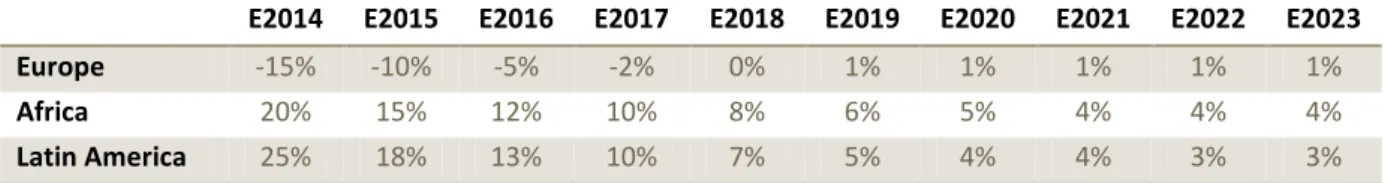
Let us start with Turnover assumptions. To reach our estimates for the growth of turnover of the Group we opted to assume growth rates for each geographic area where the Group operates.
Starting with historical values (values up to December 2013) and considering the expectations of IR department of ME (accounting for the backlog guaranteed and in the agenda for the next years), including the stabilization of European economies and a slight reduction in the huge African and Latin American growth we were able to reach the following growth rates (guaranteeing a reasonable value in 2023 as our terminal year):
E2014 E2015 E2016 E2017 E2018 E2019 E2020 E2021 E2022 E2023
Europe -15% -10% -5% -2% 0% 1% 1% 1% 1% 1%
Africa 20% 15% 12% 10% 8% 6% 5% 4% 4% 4%
Latin America 25% 18% 13% 10% 7% 5% 4% 4% 3% 3%
Table 1 – Growth rates estimated for Turnover, in the explicit period
The growth rates for Europe take into account the increase in the macroeconomic framework. We did not expect the next coming years to be the turning point, in terms of positive growth, as the value in 2013 was so negative. However, it is expected that in 2018 the turnover will not decrease as the economic situation in the countries where ME operates improves. In the following years, the expectation is that the steady state is reached. We are talking about a mature market where normally there are no huge opportunities for construction companies. Hence, we believe that a 1% growth in the terminal year is adequate.
As for African estimations, since there is a huge room for improvement in the sectors in which ME operates and adding the reputation that the company has had in Angola and has been increasing in other African countries the expectations are quite high.
ME has several projects in the agenda, regarding construction, mining, waste management, railways and highways throughout many African countries that may guarantee a continuous growth for the next years. In order to have somewhat conservative estimations, we projected a 4% growth in the last years of our explicit period with the goal of not overstating turnover even though we believed that value might be higher.
The scenario in Latin America is also quite optimistic. In 2013, ME has registered a growth in turnover of around 36%. Once again, there is a lot to be done in those countries and ME has a prestigious image from which many opportunities can be seized. For the next couple of years, ME will be working in several projects and “competing” to win many others. The
demand is very high and again for conservative reasons we predict 3% for the years preceding 2023.
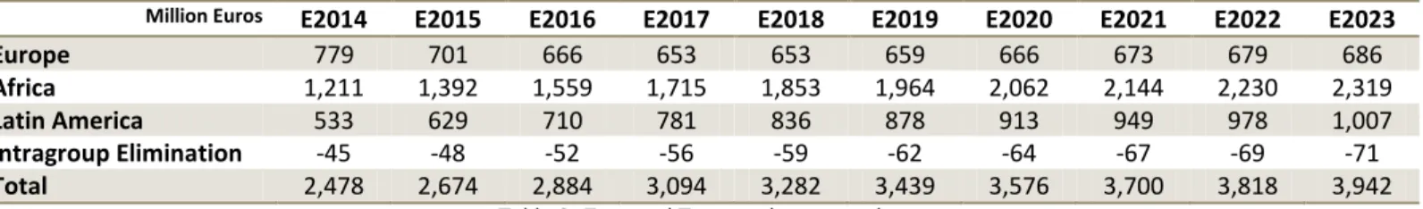
Also, we chose to forecast Intragroup Eliminations Effect based on the average weight of Intragroup Eliminations in the total value from 2011 to 2013. We applied this not only with sales but also all the other Income Statement items.
Below find the projections for turnover in absolute terms:
Million Euros E2014 E2015 E2016 E2017 E2018 E2019 E2020 E2021 E2022 E2023
Europe 779 701 666 653 653 659 666 673 679 686
Africa 1,211 1,392 1,559 1,715 1,853 1,964 2,062 2,144 2,230 2,319
Latin America 533 629 710 781 836 878 913 949 978 1,007
Intragroup Elimination -45 -48 -52 -56 -59 -62 -64 -67 -69 -71
Total 2,478 2,674 2,884 3,094 3,282 3,439 3,576 3,700 3,818 3,942
IV.1.2 Gross Profit
The assumptions used to reach ‘Gross Profit’ value relate to ‘Other Revenues’ and ‘Cost of goods sold, mat. cons. & subcontractors’.
As for ‘Other Revenues’ we assumed it grows at the same rate of ‘Sales & services rendered’ since they are directly related.
Regarding the cost of goods sold, we used its weight, as a percentage of sales, to predict the values of this item for the explicit period.
Using 2012 and 2013 values, we were able to have a better perspective on the usual weight of cost of good sales on sales for each region.
In this topic it is worthwhile mentioning that we chose to keep very similar weights to the ones verified in 2013 for all regions: Europe, Africa and Latin America, as we saw no reason to assume such value would change.
% of Sales 2013 E2014 E2015 E2016 E2017 E2018 E2019 E2020 E2021 E2022 E2023
Europe 60% 60% 60% 60% 60% 60% 60% 60% 60% 60% 60%
Africa 41% 40% 40% 40% 40% 40% 40% 40% 40% 40% 40%
Latin America 36% 36% 36% 36% 36% 36% 36% 36% 36% 36% 36%
Table 3 – Percentage of Cost of goods sold and other similar costs on Sales, by region
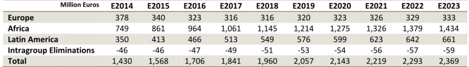
Having shown our assumptions we were now in conditions of computing Gross Profit:
Million Euros E2014 E2015 E2016 E2017 E2018 E2019 E2020 E2021 E2022 E2023
Europe 378 340 323 316 316 320 323 326 329 333
Africa 749 861 964 1,061 1,145 1,214 1,275 1,326 1,379 1,434
Latin America 350 413 466 513 549 576 599 623 642 661
Intragroup Eliminations -46 -46 -47 -49 -51 -53 -54 -56 -57 -59
Total 1,430 1,568 1,706 1,841 1,960 2,057 2,143 2,219 2,293 2,369
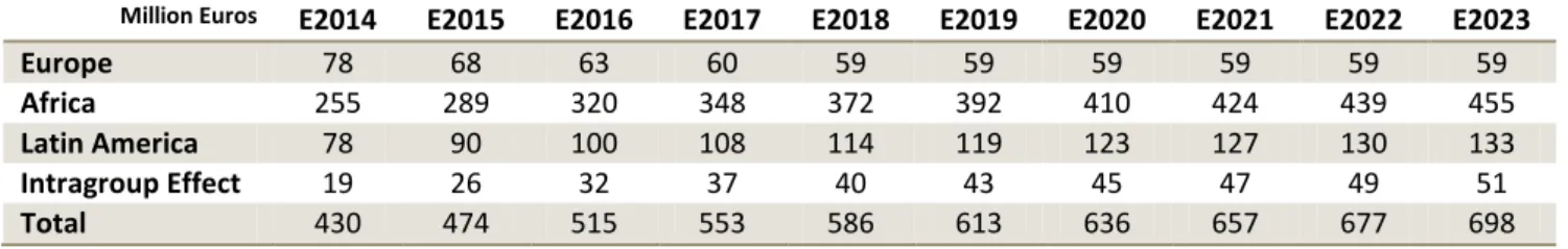
IV.1.3 EBITDA
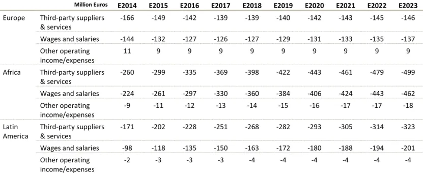
As we show in Box 3, to reach the value of EBITDA we subtracted the values of ‘Third-party suppliers and services’, ’Wages and salaries’ and add/subtract ‘Other operating income/expense’.
First of all, we assumed ‘Third-party suppliers & services’ and ‘Other operating income/(expense)’ grew with sales.
Secondly, we used the direct relation between the value of ‘Wages and salaries’ the number of employees working in ME to project the ‘Wages and salaries’ values in the explicit period. Firstly, we linearly regressed historical headcount against historical sales (using data from 2007 to 2013), being afterwards able to project headcount values for the explicit period. Again, using linear regression, we reached the linear function between the historical values of Headcount and ‘Wages and salaries’, which using the values of headcount projected, provided us with the values of ‘Wages and salaries’ for the explicit period (visit Appendix I for further detail on the methodology used).
The projected values for the items above explained were as follows:
Million Euros E2014 E2015 E2016 E2017 E2018 E2019 E2020 E2021 E2022 E2023 Europe Third-party suppliers
& services
-166 -149 -142 -139 -139 -140 -142 -143 -145 -146 Wages and salaries -144 -132 -127 -126 -127 -129 -131 -133 -135 -137 Other operating
income/expenses
11 9 9 9 9 9 9 9 9 9
Africa Third-party suppliers & services
-260 -299 -335 -369 -398 -422 -443 -461 -479 -499 Wages and salaries -224 -261 -297 -330 -360 -384 -406 -424 -443 -462 Other operating income/expenses -9 -11 -12 -13 -14 -15 -16 -17 -17 -18 Latin America Third-party suppliers & services -171 -202 -228 -251 -268 -282 -293 -305 -314 -323 Wages and salaries -98 -118 -135 -150 -163 -172 -180 -188 -194 -201 Other operating
income/expenses
-2 -3 -3 -3 -4 -4 -4 -4 -4 -4
Thus, EBITDA values were as follows:
Million Euros E2014 E2015 E2016 E2017 E2018 E2019 E2020 E2021 E2022 E2023
Europe 78 68 63 60 59 59 59 59 59 59
Africa 255 289 320 348 372 392 410 424 439 455
Latin America 78 90 100 108 114 119 123 127 130 133
Intragroup Effect 19 26 32 37 40 43 45 47 49 51
Total 430 474 515 553 586 613 636 657 677 698
IV.1.4 EBIT
Starting from EBITDA values shown in Table 6, we reached EBIT values by deducting ‘Depreciation & Amortization’ and ‘Provision and impairment losses’.
As for ‘Depreciation and amortization’, we show the assumptions and values for the group ahead in sub-chapter IV.1.6 (please check such sub-chapter to understand the rationale behind our ‘Depreciation and Amortization’ values). Here we detail the distribution of such costs by region as we need it to reach EBIT by region. We did it based on the weight of the EBITDA of each region on total EBITDA. Hence, the following results were achieved:
Million Euros E2014 E2015 E2016 E2017 E2018 E2019 E2020 E2021 E2022 E2023
Europe 21 18 17 17 17 18 20 21 22 23
Africa 69 78 88 98 108 122 136 150 164 179
Latin America 21 24 27 30 33 37 41 45 49 52
Intragroup Effect 1 2 2 2 2 2 3 3 3 3
Total 112 123 134 147 160 180 199 219 238 257
Table 7 – Depreciation and Amortization values by Region
Regarding provisions and impairment losses, we could not find direct links between this item and other Income Statement items. Due to the lack of information and since it is quite hard to predict the values of provision and impairment losses with no basis for estimation, we decided to assume that these values would be equal to a constant percentage of Sales for the explicit period. The constant percentage we used corresponds to the average of such percentage from 2007 to 2013. The average amounts to 0.9% over Sales.
Million Euros 2007 2008 2009 2010 2011 2012 2013
Prov. & Imp. Losses 9 15 6 19 35 25 17
Sales 1,402 1,869 1,979 2,005 2,176 2,243 2,314 Average
Provision % 0.7% 0.8% 0.3% 1.0% 1.6% 1.1% 0.7% 0.9%
Table 8 – Average value of historical percentage of provisions over Sales
Taking this result into account, the values for ‘Provisions and Impairment Losses’ for each region were computed (Intragroup effect not shown because its impact is not significant – less than 0.5 Million Euros in the explicit period):
Million Euros E2014 E2015 E2016 E2017 E2018 E2019 E2020 E2021 E2022 E2023
Europe 7 6 6 6 6 6 6 6 6 6
Africa 11 12 14 15 16 17 18 19 20 21
Latin America 5 6 6 7 7 8 8 8 9 9
Total 22 24 26 28 30 31 32 34 35 36
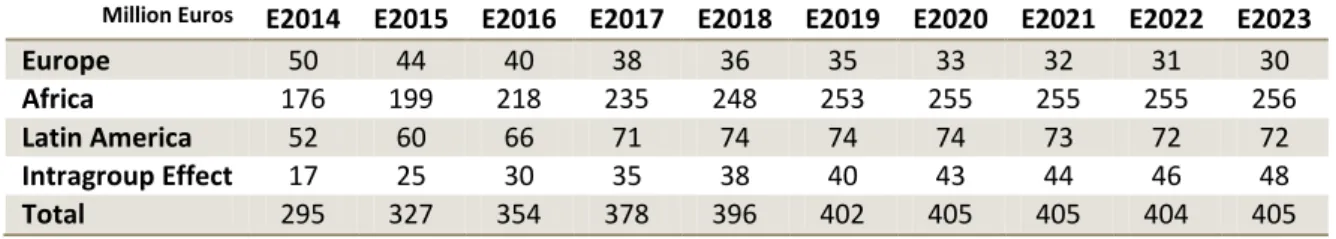
Finally, EBIT values could be computed:
Million Euros E2014 E2015 E2016 E2017 E2018 E2019 E2020 E2021 E2022 E2023
Europe 50 44 40 38 36 35 33 32 31 30
Africa 176 199 218 235 248 253 255 255 255 256
Latin America 52 60 66 71 74 74 74 73 72 72
Intragroup Effect 17 25 30 35 38 40 43 44 46 48
Total 295 327 354 378 396 402 405 405 404 405
IV.1.5 Capital Expenditure (CAPEX)
Our first assumption regarding Capital Expenditure related to the proportionality between this item and Total Sales. Since ME’s activity is asset-intensive, a lot of Capital Expenditure is required for the Group to support and generate Sales, from which we infer such relation between Sales and CAPEX.
In ME’s specific case, Intangible Assets are not as relevant to the group’s activity. So, as there was no indication that this item was expected to grow differently, we assumed that the Capital Expenditure on Intangible Assets would be equal to the one verified in 2013, for the whole explicit period.
Moving now to the Capital Expenditure on Tangible Assets, we did not assume a constant CAPEX value. We chose to assume that CAPEX value would be equal to the average value verified in the period between 2007 and 2013.
By analyzing the previous years’ CAPEX weight on sales, we could see that the average value was around 6%.
2007 2008 2009 2010 2011 2012 2013 Average
12% 12% 16% 7% 7% 6% 6% 6%
Table 11 – Capital Expenditure percentage over Sales.
As previously stated, we used the average value of CAPEX weight on Sales from previous years as our target level of CAPEX in during our explicit period.
E2014 E2015 E2016 E2017 E2018 E2019 E2020 E2021 E2022 E2023
% CAPEX on Sales 6% 6% 6% 6% 6% 6% 6% 6% 6% 6%
Table 12 – CAPEX percentage over Sales during explicit period
Using the percentages shown above, we were able to compute our CAPEX values for the explicit period.
Million Euros E2014 E2015 E2016 E2017 E2018 E2019 E2020 E2021 E2022 E2023
Capital Expenditure 161 173 186 200 212 222 231 239 246 254