Evaluating the Maximization-Maximization approach to measure default probabilities on structural credit risk models

Evaluating the Maximization-Maximization approach to

measure Default Probabilities on Structural Credit Risk

Models

Cláudia Ventura

Dissertation written under the supervision of Professor Nuno

Silva

Dissertation submitted in partial fulfilment of requirements for the

MSc in Finance, at the Universidade Católica Portuguesa,

1

A

BSTRACT

This thesis implements the Maximization-Maximization (MM) algorithm proposed by Forte and Lovreta (2012), where in the first step the expected assets rate of return and the asset volatility are estimated applying the Maximum Likelihood technique. As the firm’s assets value is not observable, the observed equity values are treated as transformed data in order to derive the log-likelihood function. In a second step, the default barrier is estimated according to the interests of shareholders, corresponding to the optimal level considered for the firm to default, and as the one that maximizes their participation. Using a sample of fifty-five companies and a time period for the estimation of one year, our results prove that estimating the expected rate of return is hard and does not provide statistically significant results, as it is dependent and highly correlated to the observed equity values. The results for the five-year default probabilities computed were most of them equal to zero or too high.

A

BSTRACT

P

ORTUGUESE

Esta tese implementa o algoritmo Maximization-Maximization (MM) proposto por Forte e Lovreta (2012), em que no primeiro passo, o retorno esperado dos ativos e a volatilidade destes são estimados aplicando a técnica da Máxima Verosimilhança. Como o valor dos ativos da empresa não é observável, os valores do capital próprio são tratados como dados transformados de forma a derivar a função log-likelihood. Num segundo passo, a barreira de incumprimento é estimada de acordo com os interesses dos acionistas, correspondendo ao nível ótimo considerado para a empresa entrar em incumprimento, bem como àquela que maximiza a participação destes. Usando uma amostra de cinquenta e cinco empresas e um período de tempo de um ano para a estimação, os nossos resultados mostram que estimar a taxa de retorno esperado dos ativos é difícil e não fornece resultados estatisticamente significativos, por ser dependente e fortemente correlacionado com os valores do capital próprio. Os resultados das probabilidades de incumprimento a cinco anos calculadas foram na maioria igual a zero ou demasiado altas.

2

A

CKNOWLEDGMENTS

The first person I would like to thank is my mother, because if it wasn’t for all her support and also financial help, I couldn’t even have started this Master program. She is and always was a fighter so I could have everything. I would also like to thank to my boyfriend and best friend Rafael for always believing in me and for being able to show me the positive side in the hard times, when sometimes I couldn’t see it for myself. And finally, I would like to thank to professor Nuno Silva for all the help he provided during these months, constantly supporting in this big challenge.

3

C

ONTENTS

1. Introduction ... 5

2. Literature Review ... 7

3. The Structural Model of Forte (2011) ... 14

4. Dataset and The MM Algorithm ... 16

4.1. Dataset ... 16 4.2. The MM Algorithm ... 17 5. Results ... 21 5.1 Parameter Estimates ... 21 5.2 Probabilities of Default ... 27 6. Conclusion ... 29 7. References ... 31 8. Appendices ... 33

4

I

NDEX OF

F

IGURES

Figure 1:Figure from Forte and Lovreta (2012) that represents the behavior of the Log-Likelihood function considering Default-to-Debt ratio (β). (P.19) Figure 2:Correlation between the asset return of the period and estimated expected asset

rate of return provided by the MM algorithm. (P.42)

Figure 3:The expected asset return provided by the MM algorithm and the equity return

calculated for the period of time considered. (P.24)

Figure 4:Correlation between the equity return on the period and the expected asset rate

of return provided by the MM algorithm. (P.24)

Figure 5:Five-year Default Probabilities (P.45)

Figure 6:Nominal debt of companies (P.46)

I

NDEX OF

T

ABLES

Table 1:Information regarding the several sectors of the sample and the corresponding

weights. (P.15)

Table 2:Comparison between the main descriptive statistics of the parameters obtained

and the ones from Forte and Lovreta (2012) (P.20)

Table 3:Results obtained from the MM algorithm application for 28 of the 55 companies

and the correspondent p-values. (P.21)

Table 4:Results obtained from the MM algorithm application for 27 of the 55 companies

and the correspondent p-values. (P.22)

Table 5:Expected asset rate of return and the stock return for all companies (P.25) Table 6:Analysis for the five-year Default Probability for Gas Natural (P.26)

Table 7:Analysis for the five-year Probability of Default (P.43)

Table 8:Analysis for the five-year Probability of Default (P.43) Table 9:Analysis for the five-year Probability of Default (P.44) Table 10:Analysis for the five-year Probability of Default (P.44)

5

1.

I

NTRODUCTION

Structural credit risk models started with Merton (1974) where it is considered that a company financed by equity and debt, specifically a pure discount bond, is only able to fulfill with its financial obligations and repay debt in the case that at debt maturity, the assets market value is higher than the nominal debt value. Otherwise, assets are sold to pay to creditors and in that case, equity holders receive nothing. This model constituted a meaningful breakthrough in credit risk modelling due to a few core motives. First, they allow the computation of the probability of default (PD) and loss given default (LGD) of a company in a single setting. Second, they provide an economic explanation for the default event of companies, and in this setting, it means default occurs in the moment assets market value is lower than a certain level, denominated the default barrier. Third, these models can be calibrated using market data, meaning they are forward looking, which is undoubtedly an advantage when comparing to credit scoring models as the Altman’s Z-score or Logit models, that are based on backward looking information. Despite the initial enthusiasm around structural models, the first applications were in fact perceived as unsuccessful. Merton’s model usually generates low credit spreads and default probabilities tends to zero as debt maturity approaches, which is not unquestionably observable. Nevertheless, several models were then presented relaxing some of Merton’s initial assumptions, and one example of these model’s assumptions is related to the fact that default can only occur at debt maturity T if the total assets value is lower than debt’s. In particular, Black and Cox (1976) introduced the possibility of early default. Following Duan (1994), several papers were written emphasizing the weaknesses of the two main methods being used to estimate Merton’s model: the system of equations and the proxy method. Some other features were taken into consideration in an attempt to overcome some of the limitations related to the structural credit risk models. Forte and Lovreta (2012) considered the probability of a firm actually surviving along the time period. This adjustment on the model seems to be appropriate as it can indeed mirror a reality of a firm. However, considering the characteristics and advantages of using the structural credit risk models when compared to others, these are indeed more appropriate as they can be calibrated using market data, meaning they are forward looking. Disadvantages or features of these models can, however, limit the accuracy of their performance, leading then to corresponding unrealistic results.

6

Some of these papers favor the use of Maximum Likelihood (ML) to estimate the model parameters. Maximum Likelihood is a statistical method that basically consists in determining the parameter values that maximize the likelihood of the data processed being actually observed. In other words, given certain data, these parameter values will maximize the likelihood function. However, in the case of models based on early default where the barrier itself has to be estimated, estimating the default barrier through the Maximum Likelihood procedure becomes an issue, since it is unstable, as Forte and Lovreta (2012) demonstrate.

The purpose of this dissertation is to implement the Maximization-Maximization (MM) algorithm suggested by Forte and Lovreta (2012). The latter breaks the model calibration in two steps. In the first step, the expected asset rate of return and the volatility of asset are estimated by applying the Maximum Likelihood technique, which is considered to have advantages when compared to other methods of parameters estimation. On the second step, the barrier level is estimated, according to the best interests of the shareholders as well as it corresponds to the level that maximizes equity holders claim. Once calibrated on a sample of fifty-five (55) non-financial European companies, the five-year probabilities of default are computed for all firms. The Maximization-Maximization (MM) algorithm proposed by Forte and Lovreta (2012) is implemented using the R program. The code is provided in Appendix B.

The remainder of this thesis is organized as follows. Section 2 analyses the literature on structural credit risk models as well as their limitations. Section 3 presents the structural credit risk model behind Forte and Lovreta (2012). Section 4 reviews the dataset used and explains the Maximization-Maximization algorithm. Section 5 describes and analyzes the results obtained from the model estimation. Finally, section 6 concludes.

7

2.

L

ITERATURE

R

EVIEW

The main methodologies to measure default risk are the credit-scoring models, reduced-form models and the structural models. Credit-scoring models basically use the company’s financial information and thus financial indicators as inputs, and in addition, each of these indicators has a weight associated which aims to reflect its relative ability to predict default. Moreover, the output generated corresponds to a numerical score which in its turn has associated a certain default probability. One of the most known scores applied to default risk is the Z-score, shaped by Edward Altman in 1968, and applied in the following way: the higher the score, the lower the likelihood of default occurring. Credit-scoring models are discussed by Altman and Saunders (1996), where they mention four approaches to develop these credit-scoring systems: the linear probability model, the logit model, the probit model and the discriminant analysis model, from which the two most used are logit and discriminant analyses. The logit model, for instance, considers accounting variables and assumes that default probability follows a logistic distribution. According to Altman and Saunders (1996), credit-scoring models have been criticized. The most impacting reasons they highlight are related to the linearity assumed in the variables when considering the linear discriminant analysis, which may not hold and therefore not being able to accurately predict default. Additionally, the fact that the models are accounting-based may result in a failure to include changes in the market conditions. Related to this, it must be emphasized that this methodology represents a significant disadvantage because these scores are backward-looking compared to the structural models, for instance, that are considered to be forward-looking.

Nevertheless, one of the main conclusions of Reisz and Perlich (2007) is that accounting-based measures, such as the Z-score, tend to present a better performance when compared to structural models if considering a timeframe of bankruptcy forecasts of one year. However, this performance decreases when the time horizon is greater. Therefore, these backward-looking measures are considered to be more relevant to predict default in a short-term basis, while forward-looking structural models are best suited to predict defaults for medium and long-terms. Altman and Saunders (1996) mention that other alternative models have been proposed in order to better predict default.

Another methodology used to predict default is the reduced-form models. They are based in different assumptions regarding the information used when compared to the structural

8

models, as pointed out by Jarrow and Protter (2004). Their main conclusion regarding the information needed for these both types of models and the consequent prediction of default, relates to the information used. Whereas reduced-form models use less information and assume that the information available is the one the market can observe, it is assumed that structural models, on the other hand, usually access to continuous observations, specifically regarding the firm’s assets and liabilities. Nevertheless, for purposes of valuation and hedging of default risk, Jarrow and Protter (2004) remark that reduced-form models should be chosen. Besides that, these models have also been given support to be implemented since there is a consensus in the literature regarding the fact that the firm’s asset value is not continuously observable in time, according not only to Jarrow and Protter (2004), but also to other authors such as Ericsson and Reneby (2005). However, Andersan and Sundaresan (2000) indicate some of the limitations of reduced-form models, being one of them the fact that they ignore the systematic risk in a portfolio of bonds.

The third category of models that are able to predict default corresponds to the structural models, which have suffered changes, as proved by the literature. The first structural bond pricing model was introduced in 1973, designated as the Black-Scholes-Merton and known as Black-Scholes model. The Black-Scholes is an option pricing model used to calculate the value of derivatives. Altman and Saunders (1996) mention that in the BSM model, the probability of a firm going bankrupt depends not only on the market value of firm assets relative to its debt, but also on the volatility of the market asset’s value. such Black and Scholes (1973) indicate that some conditions of “perfect markets” are assumed, as the option (call or put) being European, meaning it can only be exercised at the maturity, and therefore default can only happen at that time; there are no dividends paid out; the risk-free rate is known and constant throughout time; the inexistence of transaction costs in the case of buying or selling the stock or the option; and finally, the fact that total returns follow a normal distribution.

In the same setting, Merton (1974) indicates some assumptions that are considered to be simple and unrealistic. This model allows the use of BSM pricing formulas, and it is considered to be a structural model as it relates the asset structure with the default probability of the firm. One critical assumption in this model is that the firm issues only a single class of debt, specifically a zero-coupon bond, with a face value B payable at T, as previously mentioned regarding the BSM model. This is considered not to be a realistic

9

assumption as usually firms issue several bonds and assuming this, the default barrier will be determined considering only one liability. Sundaresan (2013) mentions that in case default happens, creditors take the assets of the firm. This idea is connected to the fact that Merton’s model considers that equity holders have a call option on the assets of the firm, meaning that if the assets value is higher than the debt value, then equity holders get the difference, otherwise they receive nothing. This model allows the computation of the probability of default (PD), as well as the recovery rate (RR), which provides the possibility to calculate the loss given default (LGD) measure, according to Sundaresan (2013). There is, however, a limitation this model faces that corresponds to the fact that the assets value is not observable, only the equity value is.

Forte (2011) mentions that a reason for structural models still having disadvantages and thus resulting in poor performances, has to do with how the default barriers of companies are estimated. Several developments have been done throughout time in these regards. For instance, in order to explore and relax the assumption of Merton’s model (1974) previously mentioned related to the fact that default can only happen at maturity T, Black and Cox (1976) assumed that the firm could default at any time before debt matures, in an attempt to relax this assumption considered not to be realistic. It corresponded to one of the several extensions that the original structural credit risk model owns. This approach corresponds to the so-called first-passage-time and seems to be a more realistic assumption as usually firms issue several bonds to finance themselves, allowing default events to be more flexible. In the same study, it is analyzed the effect of considering safety covenants, which are described by Black and Cox (1976) as contractual provisions that, in case the firm is underperforming, give them the right to obligate the firm to declare bankruptcy, allowing them, in turn, to obtain the ownership of the assets. Since it can happen when the asset’s value of the firm falls below a certain level, this is a way for bondholders to be protected. Furthermore, they assume the firm pays a constant dividend to stockholders using this type of contract, in contrast with Merton’s model where, on its turn, it is assumed no dividends are paid out. Besides this, it is taken into consideration the junior (or subordinated) and senior debt, given that at maturity date, senior debtholders must have been paid prior to the junior ones.

Black and Cox (1976) also demonstrate how can the default barrier be endogenously determined. However, and despite the fact that the model considers that the firm can default when the assets value becomes lower than a certain level, not providing only the

10

possibility to occur at maturity, which is already considered an advantage, it also has its disadvantages. One important limitation that is common to the Black-Scholes-Merton model corresponds to the idea that interest rates are constant, as already mentioned. This limitation is also present in Leland and Toft (1996), which corresponds to another extension of the Merton’s model. Nevertheless, after Merton (1974), there were attempts to overcome this restriction of the constant risk-free rate, as it is the example of Longstaff and Schwartz (1995) that allowed interest rates to be stochastic, applied in a first-passage-time model proposed by Black and Cox (1976).

Similar to Black and Cox (1976) that reveal there can be lower and upper boundaries given either exogenously through the contract specifications, or endogenously from an optimal decision problem, also Leland (1994) was a key contribution to Merton’s model extensions, as it presented the incorporation of taxes in a model and developed an endogenous default barrier. When the default boundary is generated endogenously, it allows the borrower, that can correspond to the shareholders of the company that is finances by equity and debt, to literally decide in which moment will the firm default. Leland (1994) also introduced bankruptcy costs, interpreted as liquidation costs. Similarly, Leland and Toft (1996)’s main conclusions consist on the fact that bankruptcy is declared under endogenous conditions and that it depends on the amount and maturity of debt, and also that the value of the assets that determine bankruptcy can be lower or higher compared to the value of debt. Another of their conclusions regarding the optimal leverage for a firm, indicates that this level depends crucially on the debt maturity, which is demonstrated to be significantly lower when the firm is financed by shorter term debt. Nonetheless, Leland and Toft (1996) assume that the company issues debt with the same principal, coupon and maturity. If one decides to define the default barrier exogenously, this could be done for instance by applying the KMV approach, which determines that the default point does not necessarily correspond to the moment when the firm’s assets are lower than the total debt, and that it is calculated considering the short-term debt and 50% of the long-term debt of the firm.

Besides the extensions that Merton’s model has caused, this KMV model also generated a fundamental impact in what concerns calculating the Expected Default Frequency (EDF), being one of its assumptions the normality of the asset returns. This approach changes the debt structure into a zero-coupon bond maturing in one year, just like Black and Scholes (1973) and Merton (1974). Expected Default Frequency is a forward-looking

11

measure of default probability that, according to Reisz and Perlich (2007), corresponds to the frequency that firms presenting the same Distance-to-Default, do indeed default. The Distance-to-Default is measured by the distance between the expected value of assets and the default point. Its calculation constitutes a great difference compared to Merton’s model regarding the computation of the probability of default. According to Crosbie and Bohn (2003), this measure corresponds to the number of standard deviations that the asset value is away from default, and to go from this to the default probability, historical default and bankruptcy frequencies are used. According to Reisz and Perlich (2007), in order to calculate the probability of default using the KMV model, a path of steps must be followed: firstly, the market value and volatility of the firm’s assets should be estimated; secondly, Distance-to-Default is measured; and finally, the default probability is calculated. Moody’s KMV model is one of the most used methods to calculate the Distance-to-Default measure. Besides, Sundaresan (2013) states that considering equity as a call option, dictated the success of the KMV model in terms of computing EDF’s. Jarrow and Turnbull (2000), for instance, compare the advantages and disadvantages of using the KMV model to estimate the probability of default. One of the strengths this model has is the fact that market information is incorporated on default probabilities when estimating the firm’s volatility and market values of assets using the market value of equity. This incorporation of information allows the model to be more reliable and updated, which according to Reisz and Perlich (2007) may lead to more accurate default predictions. Unfortunately, also this model has weaknesses that might put in danger the accuracy of these predictions, and that are pointed out by Jarrow and Turnbull (2000). One example is the fact that inputs such as the firm’s value, asset’s volatility and the expected return on the assets are not directly observed. Additionally, the use of historical data to calculate EDF is also perceived as a limitation since it is related to stationarity. This last assumption is hardly valid since there are changes in the economic cycle, hence, recessions and expansions provide different Distances-to-Default and therefore different default probabilities. Reisz and Perlich (2007) criticize this model as it implies default probabilities to be computed from historical data.

The last methodology to calculate default risk corresponds to the structural credit risk models. Also, for these, there are some controversies regarding their performance. Forte and Lovreta (2012) explain the reason why structural models still might perform poorly. They mention that determinants as the asset value of the firm and its volatility not being

12

directly observable corresponds to a limitation that these models face to present improved performances in terms of estimation. Anderson and Sundaresan (2000) additionally conclude that these models have been difficult to be implemented successfully since they also face some limitations such as the need of getting extraordinary information in terms of data. Anderson and Sundaresan (2000) state that Merton’s model is not considered to be realistic measuring default risk when the default barrier is modelled exogenously. Tarashev (2005), on the other side, accomplishes that models based on defining default barrier exogenously, usually underestimate the default risk, and are influenced by three characteristics: the leverage ratio, the recovery rate and the risk-free rate. In the same paper, it is concluded that the best methodology in terms of the models’ performance corresponds to the endogenous default model settled by Leland and Toft (1996), where probabilities of default are considered to be approximated to the default rates. In the same line of reasoning, Andersan and Sundaresan (2000) indicate that endogenously determining the default barrier has improved the structural model’s performance in general, as well as Li and Wong (2008) demonstrate that endogenous default models do indeed present higher performances compared to exogenous models. In this setting, defining the moment when default can happen, if done endogenously, then the barrier will reflect an optimal decision inside the firm, as previously pointed out. Forte and Lovreta (2012) determine, through applying the Maximization-Maximization (MM) algorithm, the default barrier reflecting the best interests of shareholders, and thus obtaining an “endogenous” barrier that is obtained also with exogenous data. This default barrier corresponds to the optimal option that maximizes the equity holders’ participation. In what regards some of the characteristics and variables that are included when studying and estimating the default barrier, Andrade and Kaplan (1998), that studied the distress costs due to financial distress for a sample of thirty-one highly leveraged transactions (HLTs), estimated that the direct costs of financial distress are approximately of 3% of the asset value, and the distress costs in companies should be between 10% and 23% of the asset firm value. In what concerns the bond maturity to be considered, and following Stohs and Mauer (1996) who studied the determinants for debt maturity, they considered the relationship between the debt maturity and the bond rating provided to the firm. One of their conclusions is precisely the fact that firms that are attributed low or high bond ratings, usually have the lowest average debt maturity. Regarding firms that have a rating of AAA, which is the top credit rating of the scale that means bonds present the best

13

creditworthiness. This financial indicator is different according to the debt maturity each firm has. In their study, the credit rating levels were applied according to the period of 1980-1989. For instance, a debt maturity of 2,34 was attributed to the AAA-rated firms.

14

3.

T

HE

S

TRUCTURAL

M

ODEL OF

F

ORTE

(2011)

Following Forte (2011), it is considered that a firm whose assets value, denoted by 𝑉𝑡,

follows a continuous diffusion process given by:

𝑑𝑉𝑡 = (𝜇 − 𝛿)𝑉𝑡𝑑𝑡 + 𝜎𝑉𝑡𝑑𝑧𝑡 (1)

where µ denotes the expected rate of return of the asset, σ corresponds to the asset return volatility, δ stands for the constant fraction of the assets that is sold to pay debtholders and shareholders, denominated as payout rate, and 𝑧_𝑡 is defined as the standard Brownian motion process.

Forte (2011) considers that the default event happens in the moment when the firm’s assets value 𝑉_𝑡 equals 𝑉_𝑏, corresponding to the critical point of default:

𝑉𝑏 = 𝛽𝑃 (2)

where β is defined as a fraction of the total debt given by P that corresponds to the nominal value. Therefore, the default barrier, which is a crucial parameter in this estimation model, is considered to be an exogenously determined fraction of nominal debt. According to Leland and Toft (1996), in case default occurs, 𝑉_𝑏 corresponds to the value of the assets that bondholders will receive.

In this setting, one can state that the company is financed by both equity and debt, where the latter is finite, thus not perpetual, and also not rolled over. Besides this, it is assumed that the firm pays a constant coupon to the bondholders. The value of the company bonds is calculated via equation (3). To note that 𝑑_𝑛 depends on both the asset’s firm value and bond’s maturity because it corresponds to a risky bond.

𝑑𝑛(𝑉𝑡, 𝜏𝑛) = 𝑐𝑛 𝑟 + 𝑒 −𝑟𝜏𝑛_[𝑝 𝑛− 𝑐𝑛 𝑟] [1 − 𝐹𝑡(𝜏𝑛)] + [(1 − 𝛼)𝛽𝑝𝑛 − 𝑐𝑛 𝑟] 𝐺𝑡(𝜏𝑛) (3)

where 𝑐𝑛 is the constant coupon, 𝑟 is the constant risk-free interest rate, 𝛼 corresponds to

the default/financial distress costs, 𝜏_𝑛 denotes the debt maturity of the firm, and 𝑝_𝑛 the principal value of debt. Appendix A provides the expressions for 𝐹_𝑡(𝜏_𝑛) and 𝐺_𝑡(𝜏_𝑛). The following function (4) determines, according to the model, that total debt equals the sum of all the bonds value for each firm:

𝐷(𝑉_𝑡) = ∑𝑁 𝑑_𝑛(𝑉_𝑡, 𝜏_𝑛)

15

For simplification reasons, in this thesis it will be assumed that companies only have one bond in their capital structure, meaning this that n is equal to 1. Therefore, all the equations and computations will assume accordingly that there is only one maturity, one principal and one coupon paid for each firm, and thus τ_n= τ, p_n= P and c_n= c respectively. Note that the value of the nominal debt for each firm corresponds to the value of the first moment (t=1) of the time period considered for the estimation. The same applies also to the coupon values as a consequence of considering only one bond for each firm. Equation (3), that calculates the value of the company’s bond, assumes therefore that debt, maturity and coupon values are constant.

The payout rate, given by δ, for each company, is calculated considering the average of the annual dividends paid in the last five years1 _{and the interest expenses paid in each}

moment of time t, divided by the sum of the nominal market capitalization and debt values, where the latter is a proxy for the asset value, which is not known ex-ante. In order to obtain one single value for the payout rate, it was computed the average of these values for the time period considered.

Moreover, in order to calculate the equity value of the firm, the debt value is subtracted from the asset’s value as equation (5) demonstrates:

𝑆_𝑡 = 𝑔(𝑉_𝑡) = 𝑉_𝑡− 𝐷(𝑉_𝑡|𝛼 = 0) (5) Where the term D (V_t |α=0) is explained by the fact that in case of default occurring, the distribution of the asset value among the debtholders and distress costs are irrelevant on the equity holder’s perspective. Notice that the assets value 𝑉_𝑡 equals the sum of the equity, debt value and bankruptcy costs considered for the firm. To elucidate also that 𝑔(𝑉𝑡), which will be better explained later, is perceived as the function that transforms

the observed equity values into the asset values.

16

4.

D

ATASET AND

T

HE

MM

A

LGORITHM

In the first part of this section, the dataset used to estimate the Forte (2011) model is described, and in the second part the Maximization-Maximization algorithm proposed by Forte and Lovreta (2012) is explained. In addition, it clarifies how is the model estimated in a two-step procedure.

4.1. D

ATASET

The sample considered in this dissertation corresponds to 55 non-financial European companies. These firms were selected considering the stock market indexes from France, Italy, Spain and Germany: CAC-40, MIB-40, IBEX-35 and DAX-30 correspondently. From the total of companies included in these indexes, some of them were excluded for a few reasons. First, similarly to Forte and Lovreta (2012), financial companies were left out as the application of structural models to these firms is usually more complex. Second, firms that presented significantly irregular amounts of dividends paid per year in the last years were similarly not included in order to accompany the line of reasoning of the model implemented which considers that the asset payout rate is constant. Furthermore, it is appropriate to have information about the expectation of this ratio in the long term. The following table summarizes the allocation among several economic sectors for the companies selected in the dataset.

Table 1- Information regarding the several sectors of the sample and the corresponding weights.

Sector Number of companies Percentage

Utilities 7 13% Energy 3 5% Industrials 11 20% Consumer Cyclicals 12 22% Consumer Non-Cyclicals 6 11% Technology 3 5% Healthcare 5 9% Basic Materials 5 9% Telecommunications Services 3 5% Sum 55 100% Sector Allocation

17

For what can be observed, the sectors that presented the highest weights are “Consumer Cyclicals” and “Industrials”.

For the time period considered, from 02-01-2015 to 31-12-2015, daily data regarding market capitalization, debt and interest expenses for all the four stock market indexes was taken out from Thomson Reuters. In line with the model that considers that the risk-free rate is constant, the risk-free interest rate considered here corresponds to the 10-year German government bond for the first day of the time period, 02-01-2015, which was 0,313%. Distress costs, 𝛼, were considered to be 20% as it is a more conservative value according to the explanation given in section 2. Finally, debt maturity of bonds, τ, was assumed to be the same for all the firms for simplicity reasons, and it corresponded to 3,312_{. All these data were used to proceed and implement the model estimation. The}

variable T is 52, corresponding to the daily data of the first day of the 52 weeks of the year considered.

4.2. T

HE

MM

A

LGORITHM

The MM algorithm consists of two steps. The first step consists of finding the values of {𝜎, 𝜇} that maximize the Log-likelihood function, provided by equation (6), fixing β. To note that the value of β in this stage corresponds to its initial guess stated as β_0. The second and last step consists on estimating the β value that maximizes the shareholders’ participation, generating an updated value for this parameter.

𝑀𝑎𝑥_{𝜎,𝜇}𝐿(𝑉̂; 𝜎, 𝜇) (6) The Maximum Likelihood of the first step of the algorithm is an estimation procedure. It provides the parameter values that make the observations of the sample the most probable to happen among the overall data set conditional on the assumed model. In our context, this translates to choosing the expected asset rate of return and asset volatility parameters that maximize the probability of observing the “observed” time series of equity values. In contrast to other methods, such as the method of moments, ML requires that one knows the density function behind the equity process. This is not known, though. One knows

2 _{This assumption was made because no data regarding the average debt maturity of the firms selected was}

available. It corresponds to the AA level bond rating according to Stohs and Mauer (1996)’s study, given in Table 4 of the paper.

18

however that equity is a function of the asset process, whose returns are normally distributed. Even though the asset process is not observed, there is a one-to-one relationship between the equity values S= {S_t; t=1,…, T} and asset values that allows the time series of equity market values to be extracted conditional on the parameters 𝜇, 𝜎 and β.

As explained, the asset values are implicit in the equity values. One can thus recover the asset values by computing the zeros of the difference between the observed equity value and the one given by the equity pricing function (Equation 5). The Newton-Raphson method was thus applied using the R function “uniroot”. This algorithm uses the first derivative of the function to find arguments that are gradually closer to the true zero of the function.

This leads Forte and Lovreta (2012) to present the below equations (7) and (8): 𝐿_𝑠(𝑆; 𝜃) = 𝐿_𝑣(𝑉̂; 𝜎, 𝜇) + ∑ ln [1 − 𝑒(− 2 𝜎2∆𝑡) ln( 𝑉_̂𝑡−1 𝑉𝑏 ) ln( 𝑉_{̂ 𝑡} 𝑉𝑏)_] 𝑇 𝑡=2 − ln[𝑃𝑛𝑑(𝜎, 𝜇)] − ∑ ln |𝜕𝑔(𝑉̂𝑡;𝜎) 𝜕𝑉̂_𝑡 | 𝑇 𝑡=2 (7) where 𝐿_𝑣(𝑉̂; 𝜎, 𝜇) = − ∑ ln 𝑉̂_𝑡−𝑇−1 2 ln (2𝜋𝜎 2 𝑇 𝑡=2 ∆𝑡) − 1 2𝜎2_∆t∗ ∑ [ln ( 𝑉̂_𝑡 𝑉̂_𝑡−1) − (𝜇 − 𝛿 − 𝑇 𝑡=2 𝜎2 2) ∆𝑡] (8)

Equation (8) results directly from assuming that asset returns are independent and normally distributed, taking logs over the product of T normal density functions.

The second and third terms of equation (7) correspond to adjustments on the survival probability that the company faces during the time period considered. Yet, 𝑃_𝑛𝑑(𝜎, 𝜇) given by equation (9) corresponds exactly to this survival probability. Duan et al. (2003) considered that taking into account the fact that the firm has survived is imperative when estimating a credit risk model. Otherwise, according to them, bias in the estimation might occur and one does not obtain accurate results if not considering this possibility that might correspond to a reality. 𝑃𝑛𝑑(𝜎, 𝜇) = ɸ [ (𝜇−𝛿−𝜎2₂)(𝑇−1)∆𝑡−ln(𝑉𝑏_𝑉 ̂ 1) 𝜎√(𝑇−1)∆𝑡 ] − 𝑒 (2 𝜎2)(𝜇−𝛿− 𝜎2 2) ln( 𝑉𝑏 𝑉̂1)_{ɸ [}(𝜇−𝛿− 𝜎2 2)(𝑇−1)∆𝑡+ln( 𝑉𝑏 𝑉_̂1) 𝜎√(𝑇−1)∆𝑡 ] (9)

19

The last term of equation (7) is recognized as the Jacobian of the transformation of the variables and defined in Appendix A.

In Equation (9), ɸ stands for the cumulative standard normal distribution function. To note that when the asset value is far from the default barrier, the probability of default (PD) is small or null. Similarly, when the value of the assets is close to 𝑉𝑏, this means

that the probability of the firm defaulting is higher.

The second step of the Maximization-Maximization algorithm is focused on estimating the optimal barrier of default for the firm. The central idea related to the estimation process used to determine the default barrier in Forte and Lovreta (2012) is based on the important fact that the firm determines its particular default policy, reflecting and representing the best interests of equity holders, maximizing their participation. Nevertheless, this only holds as long as it is represented by a constant default barrier and that this policy is mirrored in the observed equity prices. Besides, even though a barrier of default is not usually known, Forte (2011) considers it is. Furthermore, it is considered that the default barrier results from what is designated as the Optimal Default – Market Efficiency (ODME) assumption. In this second phase of the MM algorithm, the parameter values output {σ, μ} previously obtained will be considered. Therefore, when the final 𝛽 value is determined, this means that it is consistent with the Optimal Default – Market

Efficiency assumption of the model. This parameter is generated after some iterations and

stops when convergence is achieved.

While on one hand Forte (2011) allows the default barrier to be obtained from the equity prices, and thus estimating it from exogenous sources and further using it to obtain an endogenous barrier, Leland and Toft (1996) on the other hand obtained it endogenously considering the smooth-pasting condition.

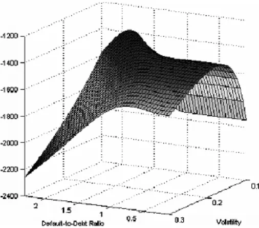
One conclusion from Forte (2011) regarding the Maximum Likelihood estimation procedure is that the estimation of the Beta parameter value is unstable when all three parameters are estimated using the Maximum Likelihood approach. In this case, the three parameters are not correctly estimated. These parameter estimation results don’t provide trustful predictions according to Figure 1 presented, that was taken from Forte and Lovreta (2012), as it demonstrates that the function often peaks at very high default-to-debt ratios, which are economically less plausible, and becomes almost flat for those barrier values that are more reasonable economically. This leads Beta estimation to

20

present a significant level of dispersion. The two-step procedure designed by Forte and Lovreta (2012) is intended to avoid this.

Figure 1- Figure from Forte and Lovreta (2012) that represents the behavior of the Log-Likelihood function considering Default-to-Debt ratio (β).

21

5.

R

ESULTS

In this section, we analyze and discuss the results obtained from the implementation of the Maximization-Maximization algorithm, such as the expected asset rate of return, the asset volatility and the critical point of default estimated. Furthermore, the default probabilities for a five-year period computed through the model are provided for the fifty-five (55) companies selected for our dataset.

5.1 P

ARAMETER

E

STIMATES

The parameter values obtained from the application of the Maximization-Maximization algorithm and the ones estimated by Forte and Lovreta (2012) are presented below in Table 2. Also, in Tables 3 and 43 _{the estimated parameter values obtained through the}

MM algorithm and the correspondent p-values are presented for each company.

Table 2 - Comparison between the main descriptive statistics of the parameters obtained and the ones from Forte and Lovreta (2012).

3 _{These results were separated in two tables so the analysis could be lighter.}

Mean Median Std. Dev. Min. Max.

β 0,564 0,447 0,259 0,161 0,985

σ 0,121 0,111 0,045 0,054 0,268

μ 0,037 0,028 0,100 -0,175 0,299

MM algorithm Forte and Lovreta (2012)

β 0,811 0,816 0,085 0,476 0,971

σ 0,163 0,150 0,091 0,041 0,542

μ 0,024 0,024 0,070 -0,190 0,239

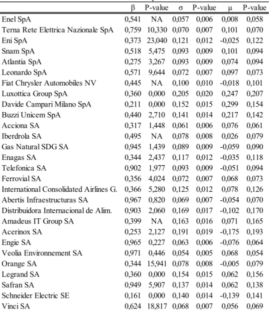
22 Table 3 – Results obtained from the MM algorithm application for 28 of the 55 companies and the correspondent

p-values.

β P-value σ P-value µ P-value

Enel SpA 0,541 NA 0,057 0,006 0,008 0,058

Terna Rete Elettrica Nazionale SpA 0,759 10,330 0,070 0,007 0,101 0,070

Eni SpA 0,373 23,040 0,121 0,012 -0,025 0,122

Snam SpA 0,518 5,475 0,093 0,009 0,101 0,094

Atlantia SpA 0,275 3,267 0,093 0,009 0,074 0,094

Leonardo SpA 0,571 9,644 0,072 0,007 0,097 0,073

Fiat Chrysler Automobiles NV 0,445 NA 0,100 0,010 -0,018 0,101

Luxottica Group SpA 0,360 0,000 0,205 0,020 0,247 0,207

Davide Campari Milano SpA 0,211 0,000 0,152 0,015 0,299 0,154

Buzzi Unicem SpA 0,440 2,710 0,141 0,014 0,217 0,142

Acciona SA 0,317 1,448 0,061 0,006 0,076 0,061 Iberdrola SA 0,495 NA 0,078 0,008 0,026 0,079 Gas Natural SDG SA 0,945 1,439 0,089 0,009 -0,059 0,090 Enagas SA 0,344 2,437 0,117 0,012 -0,035 0,118 Telefonica SA 0,902 1,977 0,093 0,009 -0,051 0,094 Ferrovial SA 0,356 4,024 0,072 0,007 0,068 0,073

International Consolidated Airlines G. 0,366 5,280 0,125 0,012 0,078 0,126

Abertis Infraestructuras SA 0,967 0,820 0,069 0,007 -0,054 0,070

Distribuidora Internacional de Alim. 0,903 2,060 0,169 0,017 -0,102 0,170

Amadeus IT Group SA 0,399 NA 0,163 0,016 0,071 0,165 Acerinox SA 0,253 2,127 0,191 0,019 -0,175 0,193 Engie SA 0,965 0,227 0,063 0,006 -0,076 0,064 Veolia Environnement SA 0,971 0,446 0,054 0,005 0,068 0,054 Orange SA 0,344 15,941 0,078 0,008 -0,005 0,079 Legrand SA 0,360 0,000 0,154 0,015 0,062 0,156 Safran SA 0,949 5,907 0,137 0,014 0,062 0,138 Schneider Electric SE 0,161 0,000 0,140 0,014 -0,139 0,141 Vinci SA 0,624 18,817 0,068 0,007 0,056 0,069

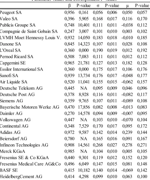
23 Table 4 – Results obtained from the MM algorithm application for 27 of the 55 companies and the correspondent

p-values.

In what the parameter values are concerned, Table 2 summarizes the main descriptive statistics considering the MM algorithm approach, enabling one to compare the results obtained in our algorithm with those found by Forte and Lovreta (2012).

As one can observe, the parameter values obtained when performing the algorithm and the ones that Forte and Lovreta (2012) present, for the same approach (MM), do not differ much. For instance, the mean of the expected asset rate of return and the asset volatility parameter values from both estimations are in fact very alike. In what β is concerned, even though the mean of the values for this parameter (0,564) is lower compared to the one from the paper (0,811), our standard deviation for these values is higher (0,259) than

β P-value σ P-value µ P-value

Peugeot SA 0,956 0,161 0,056 0,006 0,050 0,057

Valeo SA 0,396 5,905 0,168 0,017 0,116 0,170

Publicis Groupe SA 0,748 10,401 0,111 0,011 -0,038 0,112 Compagnie de Saint Gobain SA 0,247 3,007 0,101 0,010 0,003 0,102 LVMH Moet Hennessy Louis V. 0,932 14,050 0,183 0,018 -0,010 0,185

Danone SA 0,845 14,323 0,107 0,011 0,028 0,108 L'Oreal SA 0,360 0,000 0,190 0,019 0,012 0,192 Pernod Ricard SA 0,508 7,083 0,111 0,011 0,012 0,112 Capgemini SE 0,965 21,781 0,127 0,013 0,182 0,128 Essilor International SA 0,360 0,000 0,175 0,017 0,106 0,176 Sanofi SA 0,939 13,734 0,176 0,017 -0,048 0,177 Air Liquide SA 0,520 11,041 0,155 0,015 -0,062 0,157 Deutsche Telekom AG 0,445 NA 0,095 0,009 0,046 0,096 Deutsche Post AG 0,378 8,928 0,116 0,011 -0,082 0,117 Siemens AG 0,359 9,765 0,107 0,011 -0,089 0,108 Bayerische Motoren Werke AG 0,470 17,856 0,082 0,008 -0,013 0,083 Daimler AG 0,270 14,578 0,094 0,009 -0,007 0,095 Volkswagen AG 0,447 NA 0,103 0,010 -0,070 0,104 Continental AG 0,348 7,529 0,170 0,017 0,095 0,172 Adidas AG 0,972 9,587 0,142 0,014 0,239 0,144 Beiersdorf AG 0,780 NA 0,165 0,016 0,091 0,167 Infineon Technologies AG 0,908 14,561 0,268 0,027 0,278 0,271 Merck KGaA 0,985 NA 0,104 0,010 0,005 0,105

Fresenius SE & Co KGaA 0,440 9,301 0,119 0,012 0,152 0,120 Fresenius Medical Care AG&Co 0,496 6,049 0,147 0,015 0,081 0,148

BASF SE 0,415 10,182 0,140 0,014 -0,069 0,142

HeidelbergCement AG 0,414 4,298 0,099 0,010 0,063 0,100 Parameter values and correspondent P-values

24

theirs (0,085). In addition, the highest value obtained for the parameter is very similar comparing to the one Forte and Lovreta (2012) obtained in the estimation process. Besides this, our results for this parameter values are in line with the conclusion obtained from the paper stating that, when considering the MM approach, default barrier is equal or lower to the nominal debt value since we haven’t obtained, in our estimation process, any value for β equal or higher than one. In addition, we can also verify that Forte and Lovreta (2012) obtained negative values for the expected asset rate of return, similarly to the ones obtained in this thesis. Therefore, one can conclude that in general the overall results are comparable.

Tables 3 and 4 present the estimated values obtained in the algorithm for the fraction of default barrier (β), asset volatility and expected asset rate of return. These results seem to be reasonable in general terms as for instance in what regards the values estimated for the asset volatility. The highest value for this parameter corresponds to the one for Infineon Technologies AG company with 26,84%. In what the expected asset return rate parameter is concerned, one can see that there are some negative values obtained among the fifty-five (55) companies. Regarding the β parameter results, these did vary between 0,161 and 0,985. Both tables also present the p-value correspondent to each of the parameter values estimated. One can state that p-values for the asset volatility parameter demonstrate that these results are statistically significant since all of them are lower than 0,05. Nevertheless, for the expected asset rate of return the same conclusion cannot be made, since all firms present p-values that indicate the results obtained for this parameter are statistically insignificant. Regarding this parameter the high p-values observed were already expected.

Related to the results just described, there is a relevant and appropriate note which is related to the fact that estimating the expected asset rate of return is considered to be extremely hard. Its estimation is influenced due to a few motives. The first one has to do with the fact that this parameter basically corresponds to the implicit asset return of the period estimated in the model, as shown in Figure 2 provided in Appendix C. Following to this, the expected asset return rate of the period is also sensitive and strongly correlated with the equity returns observed for the time period. This can be observed from Figures 3 and 4, where specifically in Figure 4 there is evidence of a correlation coefficient R^2 equal to 0,787. Additionally, Table 5 illustrates that in most cases, when the stock return is negative, this leads to negative values for the expected asset rate of return. In this thesis,

25

we can perceive as a limitation for the results obtained the fact that the estimation period considered is very short (one year). In conclusion, not only do the p-values correspondent to the expected asset rate of return obtained prove this estimation not to be trustful, and thus not accurate, but also these Figures do.

Figure 3- The expected asset return provided by the MM algorithm and the equity return calculated for the period of time considered.

Figure 4 -Correlation between the equity return on the period and the expected asset rate of return provided by the MM algorithm.

In concluding terms, μ should be interpreted as the expected asset rate of return. The method, though, is considering the equity return on the period, which was not supposed.

26

This parameter should always be positive value and higher than the risk-free interest rate, which is something that is not observable in these results. This suggests that an alternative method, such as CAPM, should be used to estimate the expected asset rate of return.

27

5.2 P

ROBABILITIES OF

D

EFAULT

The probabilities of default were computed using the parameter values obtained in the MM algorithm. Figure 5 provided in Appendix C presents the estimated five-year default probabilities for each firm.

As one can see, most of them present values that are equal or extremely close to zero, and on the other side, a few of them have very high estimates for the probability of default for a five-year horizon. This is mainly due to the reasons already pointed out regarding the struggle on estimating the expected assets return rate, which will in turn influence the computation of this credit risk measure that is the default probability, since it is being applied the estimated parameter values obtained from the algorithm, including the expected assets rate of return.

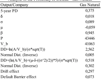
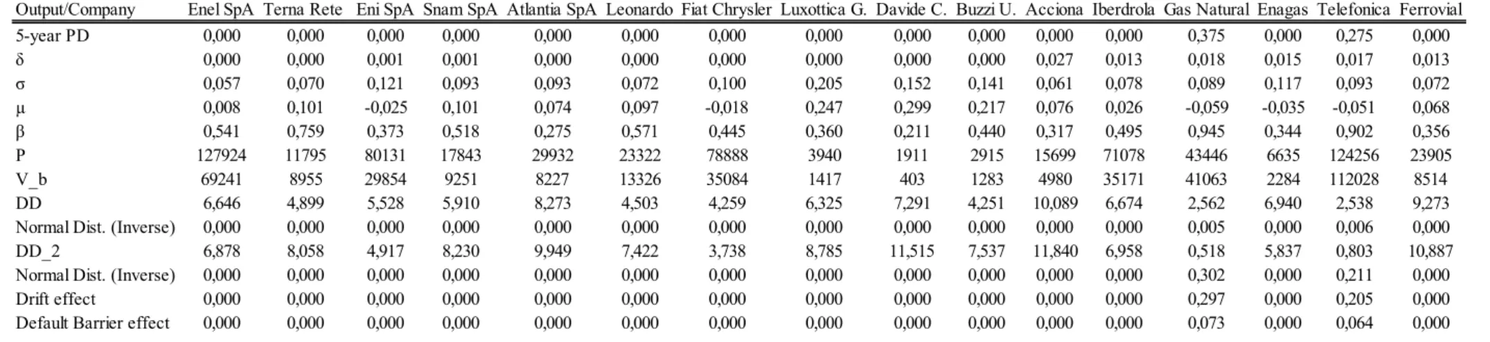
For those companies that present high values for the default probabilities computed, what is expected is that they present low Distance-to-Default (DD) values associated. In the same reasoning, for those that have low or null probabilities of default (PD), it is expectable that the Distance-to-Default measure is larger, meaning the company is far from the critical point of default. Gas Natural company is a good example to provide and to illustrate this, as the company presents a probability to defaulting in the next five years of 37,48%.Table 6 provides a summary of the results about Gas Natural. Tables 7 to 10 in Appendix C contain the same information but for all the companies considered and Figure 6 presents the nominal value of debt for all companies.

Table 6 – Analysis for the five-year Default Probability for Gas Natural

Output/Company Gas Natural

5-year PD 0,375 δ 0,018 σ 0,089 µ -0,059 β 0,945 P 43446 V_b 41063 DD=ln(A/V_b)/(σ*sqrt(T)) 2,562

Normal Dist. (Inverse) 0,005

DD=(ln(A/V_b)+(µ-δ-((σ^2)/2))*5)/(σ*sqrt(T)) 0,518

Normal Dist. (Inverse) 0,302

Drift effect 0,297

Default Barrier effect 0,073

28

It is worth mentioning though, before analyzing the information, that this estimation includes both the trajectory of the firm’s assets value along these years and therefore considering the likelihood of defaulting at any point in time, as well as the probability of defaulting at debt maturity. Given this principle, it is expected that this estimated value is higher than if only bearing in mind the possibility of defaulting at maturity. The first thing one can observe is that the expected asset rate of return for this firm is negative, corresponding to approximately -6%, and this can partially justify the probability of default obtained by the model.

Secondly, one can calculate the Distance-to-Default4 _{ignoring the drift from equation (9)}5

as Sun et al. (2012) did. The option of ignoring the drift seems to be appropriate in this case since as already explained, when one estimates the expected asset rate of return, it does not provide confident results. This results in a Distance-to-Default equal to 2,562. If we evaluate the negative of the normal distribution of this value, we obtain 0,005. On the other side, if we compute the Distance-to-Default considering the drift that previously ignored, we obtain a smaller value, equal to 0,518. This on itself allows us to conclude that if considering the drift, the company is closer to the default point. When computing the negative of the normal distribution of that value, we obtain 0,302. This 30,2% corresponds to the default probability in the five-year horizon if the model did not consider a default barrier. Besides, when we analyze and subtract the value 0,302 to 0,375, the difference corresponds to the barrier effect (7,3%). It is important to note that the barrier effect is exponential to the expected asset rate of return parameter estimated. This results from the fact that, if everything remains the same, when a default barrier exists, it potentializes the increase of the default probabilities. The remaining difference until completing the 37,5% (Probability of Default) corresponds to the drift effect (26,7%6_).

When analyzing results for companies with high probabilities of default, one can observe results follow the same line of reasoning.

In what regards the null default probabilities that were obtained for most companies of the sample, what we can conclude is that these results are highly influenced from the estimation of the expected asset return rate, as it was already justified and demonstrated.

4 _{This equation is given by: Ln(A_0/V_b)/ (𝜎*√5)}

5 _{The “drift” in this equation consists in the first part of the numeration, where the payout rate is subtracted}

to the asset rate of return.

6 _{Obtained from the difference between the negative normal distributions of the Distance-to-Default (DD)}

29

6.

C

ONCLUSION

The purpose of this thesis was first to estimate the expected asset rate of return and the asset volatility parameters through the application of the Maximum Likelihood technique. As the firm’s assets value are not usually known, Forte and Lovreta (2012) consider the observed equity values as transformed data, allowing then the ML estimation to derive the log-likelihood function using the already transformed equity values. In what the expected asset rate of return is concerned, the main conclusion one can take from this has to do with the struggle with its estimation process. The results obtained do not allow one to truly rely on them, due to several reasons that were previously illustrated. The first one is related to the p-values that were obtained upon the model estimation, which demonstrate that there is a large confidence interval for this parameter. Secondly, our estimates on the expected asset rate of return seem to be capturing the actual equity returns observed for the period under analysis. Ideally, this should not occur as the expected asset return parameter should be interpreted as the rate of return investors demand for buying the firm asset. Independently of the rate of return observed in any specific period, this parameter should correspond to the risk-free interest rate plus a positive risk premium. In what concerns the asset volatility, the same conclusion is not applicable, however. This estimated parameter presents lower p-values comparing to the ones obtained from the expected asset return, being all of them less than 0,05, which in this case allows one to conclude that these parameter results are statistically significant.

In a second step, the default barrier of each firm was then computed taking into consideration the values for the parameters previously obtained. This default barrier is considered to be the optimal and according to the best interests of shareholders as it corresponds to the one that maximizes their equity participation. Forte and Lovreta (2012) concluded that this would be a more suitable method to estimate the default barrier because, as it is demonstrated in their study, when one estimates the three parameters simultaneously by Maximum Likelihood, it is difficult to accurately estimate the Default-to-Debt ratio (β). Thus, performing this second maximization procedure for this parameter on the algorithm using the set of parameters previously estimated {σ, μ}, corresponds to the crucial innovation on their study.

Regarding the five-year default probabilities computed using these parameter values, one can conclude that the results that were obtained are not accurate. Most of the default

30

probabilities obtained for the companies are in fact null. In these cases, this happened because this probability of default measure is influenced by the estimated expected rate of return on the assets. There were, however, a few firms that presented high default probabilities as for instance Gas Natural did. The results obtained for the default probabilities for these companies are a consequence first, of the fact that when a default barrier exists, it increases on itself the probability of default occurring, and can secondly be a result from the negative expected asset returns that was obtained for these companies, that is on its turn a consequence of the estimation process of the parameter. Besides this, the drift effect later calculated, ignoring the first passage time, is increased by the fact that one is considering and computing five-year default probabilities. This would not be expectable to happen if computing instead for one-year time horizon.

In this thesis, for simplicity reasons, several assumptions were made. These assumptions correspond possibly to crucial limitations in what regards the performance of the model estimation and consequently on the results obtained. Some examples of these assumptions correspond to the nominal debt and coupon values that were considered to be constant in the time period considered. It was also assumed that each company had one single bond available, which does not also correspond to the reality of the companies as they usually issue several bonds in order to finance and raise capital. Another crucial constraint on this thesis was indeed the very short time period considered to proceed with the estimation. This fact has undoubtedly influenced negatively the results obtained for the expected asset return rate parameter values. Nonetheless, one does not know the exact time interval needed in order to obtain statistically significant values for this parameter. Therefore, in future research, it can be recommended that this data characteristic is considered upon the model estimation in order to obtain more accurate results. Besides this, there is one feature of the model considered by Forte and Lovreta (2012) that could also be a partial negative influence on the results obtained from the estimation process, which is related to the dividends distribution policy assumed for companies. In the model, it is only considered, in order to calculate the payout rate, the interest expenses and the dividends that were paid. In fact, it could also be considered the possibility of the company buying their own stock.

31

7.

R

EFERENCES

Altman, Edward I.; Saunders, Anthony (1996): Credit Risk Measurement: Developments over the last 20 years. In Journal of Banking & Finance.

Anderson, Ronald; Sundaresan, Suresh (2000): A comparative study of structural models of corporate bond yields: An explanatory investigation. In Journal of Banking & Finance. Andrade, Gregor; Kaplan, Steven N. (1998): How Costly Is Financial (Not Economic) Distress? Evidence from Highly Leveraged Transactions That Became Distressed. In The

Journal of Finance, Vol. 53, No. 5. pp. 1443-1493.

Black, Fischer; Cox, John C. (1976): Valuing Corporate Securities: Some effects of Bond Indenture provisions. Vol. XXXI, no. 2. In The Journal of Finance, pp. 351-367.

Black, Fischer; Scholes, Myron (1973): The Pricing of Options and Corporate Liabilities. In The Journal of Political Economy, Vol. 81, No. 3, pp. 637-654.

Crosbie, Peter; Bohn, Jeff (2003): Modeling Default Risk.

Duan, Jin-Chuan; Gauthier, Geneviève; Simonato, Jean-Guy; Zaanoun, Sophia (2003): Estimating Merton’s Model by Maximum Likelihood with Survivorship Consideration. Ericsson, Jan; Reneby, Joel (2005): Estimating Structural Bond Pricing Models. In The

Journal of Business, Vol. 78. No 2, pp.707-735

Forte, Santiago (2011): Calibrating structural models: a new methodology based on stock and credit default swap data, Quantitative Finance, 11:12, pp. 1745-1759, DOI:

10.1080/14697688.2010.550308

Forte, Santiago; Lovreta, Lidija (2012): Endogenizing exogenous default barrier models: The MM algorithm. In Journal of Banking & Finance, pp.1639-1652.

Jarrow, Robert A.; Protter, Philip (2004): Structural versus Reduced Form Models: A new information based perspective. In Journal of Investment Management, Vol. 2, No. 2, pp. 1-10

Jarrow, Robert A.; Turnbull, Stuart M. (2000): The intersection of market and credit risk. In Journal of Banking & Finance, pp. 271-299.

32

Leland, Hayne E. (1994): Corporate Debt Value, Bond Covenants, and Optimal Capital Structure. In Journal of Finance, Volume 49, Issue 4, pp. 1213-1252.

Leland, Hayne E.; Toft, Klaus Bjerre (1996): Optimal Capital Structure, Endogenous Bankruptcy, and the Term Structure of Credit Spreads. In The Journal of Finance, Vol. 51, No. 3, pp. 987-1019.

Li, Leung Ka; Wong, Hoi Ying (2008): Structural Models of Corporate Bond Pricing with Maximum Likelihood Estimation. In Journal of Empirical Finance, pp. 751-777.

Longstaff, Francis A.; Schwartz, Eduardo S. (1995): A Simple Approach to Valuing Risky Fixed and Floating Rate Debt. In The Journal of Finance, Vol. 50, No. 3, pp. 789-819.

Merton, Robert C. (1974): On the Pricing of Corporate Debt: The Risk Structure of Interest Rates. In The Journal of Finance, Vol. 29, No. 2, pp. 449-470

Reisz, Alexander S.; Perlich, Claudia (2007): A market-based framework for bankruptcy prediction. In Journal of Financial Stability 3, pp. 85-131.

Stohs, Mark Hoven; Mauer, David C. (1996): The Determinants of Corporate Debt Maturity Structure. In The Journal of Business, Vol. 69, No. 3

Sundaresan, Suresh (2013): A Review of Merton’s Model of the Firm’s Capital Structure with its Wide Applications. In The Annual Review of Financial Economics, 5:5.1-5.21. Sun, Zhao; Munves, David; Hamilton, David T. (2012): Public Firm Expected Default Frequency (EDFTM) Credit Measures: Methodology, Performance, and Model Extensions

33

8.

A

PPENDICES APPENDIX A 𝐹𝑡(𝜏𝑛) = ɸ[ℎ1𝑡(𝜏𝑛)] + ( 𝑉_𝑡 𝑉_𝑏) −2𝑎 ɸ[ℎ2𝑡(𝜏𝑛)] (21) 𝐺𝑡(𝜏𝑛) = ( 𝑉𝑡 𝑉𝑏) −𝑎+𝑧 ɸ[𝑞1𝑡(𝜏𝑛)] + ( 𝑉𝑡 𝑉𝑏) −𝑎−𝑧 ɸ[𝑞2𝑡(𝜏𝑛)] (22) 𝑞1𝑡 = −𝑏𝑡− 𝑧𝜎2𝜏𝑛 𝜎√𝜏𝑛 𝑞2𝑡 = −𝑏𝑡+ 𝑧𝜎2𝜏𝑛 𝜎√𝜏𝑛 ℎ1𝑡 = −𝑏𝑡− 𝑎𝜎2𝜏𝑛 𝜎√𝜏𝑛 ℎ2𝑡 = −𝑏𝑡+ 𝑎𝜎2𝜏𝑛 𝜎√𝜏𝑛 𝑎 =𝑟 − 𝛿 − 𝜎2 2 𝜎2 𝑏𝑡 = 𝑙𝑛 ( 𝑉𝑡 𝑉𝑏 ) 𝑧 =√(𝑎𝜎 2_{) + 2𝑟𝜎}2 𝜎2 𝜕𝑔(𝑉𝑡;𝜎) 𝜕𝑉𝑡 = 𝜕[𝑉𝑡−𝐷(𝑉𝑡|𝛼 = 0; 𝜎)] 𝜕𝑉𝑡 = 1 − ∑ 𝜕𝑑𝑛(𝑉𝑡|𝛼 = 0; 𝜎) 𝜕𝑉𝑡 𝑁 𝑛=1 (23) 𝜕𝑑𝑛(𝑉𝑡|𝛼 = 0; 𝜎) 𝜕𝑉𝑡 = −𝑒−𝑟𝜏𝑛_(𝑝 𝑛− 𝑐𝑛 𝑟) 𝜕𝐹𝑡(𝜏𝑛) 𝜕𝑉𝑡 + (𝛽𝑝𝑛− 𝑐𝑛 𝑟) 𝜕𝐺𝑡(𝜏𝑛) 𝜕𝑉𝑡 𝜕𝐹𝑡(𝜏𝑛) 𝜕𝑉𝑡 = 𝑓(ℎ1𝑡) 𝜕ℎ1𝑡 𝜕𝑉𝑡 − [2𝑎 𝑉𝑏 (𝑉𝑡 𝑉𝑏 ) −2𝑎−1 ] ɸ(ℎ2𝑡) + ( 𝑉𝑡 𝑉𝑏 ) −2𝑎 𝑓(ℎ2𝑡) 𝜕ℎ2𝑡 𝜕𝑉𝑡 𝜕𝐺_𝑡(𝜏_𝑛) 𝜕𝑉_𝑡 = [ −𝑎+𝑧 𝑉_𝑏 ( 𝑉_𝑡 𝑉_𝑏) −𝑎+𝑧−1 ] ɸ(𝑞1𝑡) + ( 𝑉_𝑡 𝑉_𝑏) −𝑎+𝑧 𝑓(𝑞1𝑡) 𝜕𝑞_1𝑡 𝜕𝑉_𝑡 + [ −𝑎−𝑧 𝑉_𝑏 ( 𝑉_𝑡 𝑉_𝑏) −𝑎−𝑧−1 ] ɸ(𝑞2𝑡) + (𝑉𝑡 𝑉𝑏) −𝑎−𝑧 𝑓(𝑞2𝑡) 𝜕𝑞2𝑡 𝜕𝑉𝑡 𝜕ℎ1𝑡 𝜕𝑉𝑡 =𝜕ℎ2𝑡 𝜕𝑉𝑡 =𝜕𝑞1𝑡 𝜕𝑉𝑡 =𝜕𝑞2𝑡 𝜕𝑉𝑡 = − 1 𝑉𝑡𝜎√𝜏𝑛

34

APPENDIX B

#Declare estimation period T<-52 NumberFirms<-55 EquityMatrix<-read_excel("C:/Users/claud_000/Desktop/Finance Master/TESE/DADOS.xlsx",sheet = "MarketCap") EquityMatrix<-as.matrix(EquityMatrix[1:T,2:(NumberFirms+1)]) NominalDebt<-read_excel("C:/Users/claud_000/Desktop/Finance Master/TESE/DADOS.xlsx",sheet = "NominalDebt") NominalDebt<-as.matrix(NominalDebt[1:T,2:(NumberFirms+1)]) OtherData<-read_excel("C:/Users/claud_000/Desktop/Finance Master/TESE/DADOS.xlsx",sheet = "OtherData") OtherData<-as.matrix(OtherData[1:6,2:(NumberFirms+1)]) Liab<-OtherData[3,] Coupon<-OtherData[2,] Payout<-OtherData[1,] Tau<-3.31 Alpha<-0.2 RF<-0.00313 year<-1 #Latent= 1 observation

derivh_1t <- function(V_t, sigma, Tau) {(-1)/(sigma*V_t*sqrt(Tau))}

derivh_2t <- function(V_t, sigma, Tau) {(-1)/(sigma*V_t*sqrt(Tau))}

35

derivq_2t <- function(V_t, sigma, Tau) {(-1)/(sigma*V_t*sqrt(Tau))}

derivF <- function(Latent, Beta, P, r, payout, sigma, Tau) {

(dnorm(h_1t(V_t=Latent, Beta, P, r, payout, sigma, Tau))*derivh_1t(V_t=Latent, sigma, Tau))+

-((2*a(r, payout, sigma)/V_b(Beta, P))*((Latent/V_b(Beta, P))^(-2*a(r, payout, sigma)-1)))*pnorm(h_2t(V_t=Latent, Beta, P, r, payout, sigma, Tau))+

(((Latent/V_b(Beta, P))^(-2*a(r, payout, sigma)))*dnorm(h_2t(V_t=Latent, Beta, P, r, payout, sigma, Tau))*derivh_2t(V_t=Latent, sigma, Tau))

}

derivG <- function(Latent, Beta, P, r, payout, sigma, Tau) {

((((-a(r, payout, sigma)+z(r, payout, sigma))/V_b(Beta, P))*((Latent/V_b(Beta, P))^(-a(r, payout, sigma)+z(r, payout, sigma)-1)))*pnorm(q_1t(V_t=Latent, Beta, P, r, payout, sigma, Tau)))+

+(((Latent/V_b(Beta, P))^(-a(r, payout, sigma)+z(r, payout, sigma)))*dnorm(q_1t(V_t=Latent, Beta, P, r, payout, sigma, Tau))*derivq_1t(V_t=Latent, sigma, Tau))+

+((((-a(r, payout, sigma)-z(r, payout, sigma))/V_b(Beta, P))*((Latent/V_b(Beta, P))^(-a(r, payout, sigma)-z(r, payout, sigma)-1)))*pnorm(q_2t(V_t=Latent, Beta, P, r, payout, sigma, Tau)))+

+(((Latent/V_b(Beta, P))^(-a(r, payout, sigma)-z(r, payout, sigma)))*dnorm(q_2t(V_t=Latent, Beta, P, r, payout, sigma, Tau))*derivq_2t(V_t=Latent, sigma, Tau))

}

derivD <- function(Latent,c, Beta, P, r, payout, sigma, Tau) {

-exp(-r*Tau)*(P-c/r)*derivF(Latent, Beta, P, r, payout, sigma, Tau)+(Beta*P-c/r)*derivG(Latent, Beta, P, r, payout, sigma, Tau)

}

derivS <- function(Latent,c, Beta, P, r, payout, sigma, Tau) { (1-derivD(Latent,c, Beta, P, r, payout, sigma, Tau))

36

RecoverAsset<-function(Beta, sigma){ AssetProxy<-1:T

for(i in 1:T){

AssetProxy[i]<-Vfunction(Beta, sigma, TimeMoment=i) }

return(AssetProxy) }

Vfunction <- function(Beta, sigma, TimeMoment) {

uniroot(f = FindV, interval=c(EquityMatrix[TimeMoment, firm],

EquityMatrix[TimeMoment, firm]+2*NominalDebt[TimeMoment, firm]), extendInt="downX", Beta, sigma, TimeMoment)$root

}

#x corresponds to the asset value

FindV <- function(x, Beta, sigma, TimeMoment) {

EquityMatrix[TimeMoment, firm]-S_t(V_t=x, c=Coupon[firm], Beta=Beta, P=NominalDebt[TimeMoment,firm], r=RF, payout=Payout[firm], sigma=sigma, Tau=Tau)

}

#Assumption:Tau is constant and individual bonds won't be considered-> only one bond outstanding

a <- function(r, payout, sigma) {(r-payout-((sigma^2)/2))/(sigma^2)} #r= risk-free rate

#payout= fraction of the assets paid out to investors #sigma= volatility of assets return

V_b <- function(Beta, P) {Beta*P}

#P= nominal value of total debt issued= value of the bond; known input #Beta= fraction of P; estimated iteractivelly; should assume starting value