Quantification of greenhouse gas emissions from the
biodegradation of garden waste
Joana Marinheiro
Dissertação para obtenção do grau de Mestre em
Engenharia do Ambiente
Orientadores: Professora Cláudia Cordovil
Doutor Nicholas Cowan
Júri:
Presidente: Doutora Rita do Amaral Fragoso, Professora Auxiliar do(a) Instituto Superior de Agronomia da Universidade de Lisboa
Vogais: Doutora Ute Maria Skiba, Professora do(a) Centre for Ecology and Hydrology Doutora Cláudia Saramago de Carvalho Marques dos Santos Cordovil, Professora Auxiliar do(a) Instituto Superior de Agronomia da Universidade de Lisboa
II
Acknowledgments
All the personal growth underlying in this study is because of all the help it was given to me during this process.
I have to thank to my supervisor from my university, Dr Claudia Cordovil, who gave me the opportunity to learn and grow in this area along with other alike professionals in many different occasions. Among these professionals, I also want to give a special recognition to my supervisor at CEH, Dr. Nicholas Cowan, who spent much of his time teaching me new tools and answering my incessant questions. I’m also very grateful to all the guidance and good advice given to me by Dr. Ute Skiba. I would also like to thank to all the assistance given to me in the field taking measurements or in the laboratory by Dr. Julia Drewer, Jocelyn Brichet, Colin Bache, João Serra and Martim Cruz.
Because taking a master degree doesn’t make one grow only academically, but personally too, I have also to thank to the endless support given by my family. Especially my mother and father, who were my pillars of safety and perseverance when confronting the adversities along my academic path. I’m also very thankful to Bernardo, who is always there to help me and making me as happy as I can be. Last and not least to my friends, for making all the journey more lightweight with the fun times provided.
III
Abstract
The primary aim of this study was to quantify garden waste potential for GHG emissions (with focus on CH4 and N2O); and to identify relationships between these GHG emissions and
meteorological variables in different climates. The study was carried out in two countries with contrasting climates and soil structures: Portugal with a Mediterranean climate and Scotland with a hyperoceanic climate.
A closed static chamber methodology was used for measure N2O and CH4 gaseous flux in
three types of treatments installed in containers kept outdoors: S with soil; S+GW with soil and garden waste layered on top; and GW with only garden waste. The range of N2O fluxes varied
on a log-normal scale, ranging from slightly negative values to very high values (3 orders of magnitude). With the exception of the “control” S treatments (maximum flux of 0.54 N2O nmolm -2s-1 at both sites).
The percentage of the emitted CO2 equivalent (CO2eq) from the original C content applied to
the treatments as garden waste indicates the overall impact on emissions of the composting process. Based on CO2eq global warming potential (GWP) multipliers stated by the IPCC
(2014) (25 for CH4 and 298 for N2O), Portugal emitted 28.47% from the treatment S+GW and
11.26% from GW, while the majority of the C remained on soils (>70%). Scotland’s treatment S+GW had a lower CO2eq emission of 11.99%, with 58.47% emitted from the GW treatment.
These results show that the overall impact on GWP of composting varies dramatically depending on management, and that CO2 is being converted into considerably high quantities
of longer lived GHGs like CH4 and N2O.
Cumulative CH4 flux measurements showed sequestration in Portugal and emissions in
Scotland, the effects were more pronounced in treatment S for both sites (-210.85 and 209.0519 mgCH4m-2d-1, respectively). The garden waste diminished the emissions for
Scotland and hindered the sequestration for Portugal.
The contribution of weather conditions from each site was significant and very different relatively to the behaviour of each GHG. Portugal had constant moderate/high temperatures with peaks of rain which stimulated the GHG; Scotland on the other hand had constant rain with low temperatures with occasional rises which was the controlling factor stimulating the GHG.
IV
Resumo
O objetivo principal deste estudo foi quantificar a emissão de gases efeito estufa provenientes de resíduos de jardinagem (ou resíduos verdes), com especial foco nos gases CH4 e N2O, e
avaliar o comportamento destes mesmos gases consoante diferentes variáveis meteorológicas sob diferentes climas. O estudo realizou-se em dois países com climas contrastantes e com diferentes tipos de solos: Portugal com um clima Mediterrânico e Escócia com um clima hiperoceanico.
A metodologia utilizada para a medição dos gases N2O e CH4 foi através de camaras estáticas
fechadas para três tratamentos diferentes em condições do exterior: S com solo; S+GW com solo e resíduo verde no topo; e GW com resíduo verde, unicamente. O alcance dos fluxos de N2O, numa escala log-normal, variou de valores ligeiramente negativos a valores altos (3
ordens de magnitude). Com a exceção do tratamento S (0,54 N2O nmolm-2s-1, para ambos
sítios).
A percentagem de CO2 equivalente emitido da quantidade de C proveniente dos resíduos
verdes aplicados indica que houve emissões de GEE distintos do CO2 provenientes deste
resíduo. O tratamento S+GW em Portugal emitiu 28.47% e o tratamento GW 11.26 %, a maioria do C permaneceu no solo (>70%) para ambos os casos, no entanto indica a possibilidade do solo também ter ajudado na sua emissão. O tratamento S+GW na Escócia teve uma menor emissão de 11.99% face aos 58.47% do tratamento GW o qual estará possivelmente relacionado com as altas emissões de N2O que teve, como indicado no seu
factor de emissão (4.35%).
Observou-se um sequestro no fluxo acumulado de CH4 em Portugal e, contrariamente, na
Escócia houve emissões deste gás, sendo mais acentuadas no tratamento S (-210,85 e 209,05 mgCH4m-2d-1, respetivamente) e ao juntar o resíduo verde (S+GW) houve uma
atenuação tanto para o sequestro em Portugal como para emissões na Escócia.
A contribuição das condições climáticas foi significativa em ambos os locais, e bastante diferente relativamente ao comportamento de cada GEE. Portugal apresentou temperaturas moderadas a elevadas com dias secos seguidos de picos de chuva estimulando assim a emissão dos GEE. A Escócia, por outro lado, contou com chuva constante e com temperaturas relativamente baixas com aumentos ocasionais sendo este o fator que mais estimulou os GEE.
V
Resumo alargado
Uma sociedade em constante crescimento tem a si associado um crescimento, à mesma escala, da quantidade de resíduos produzidos. Como tal, é necessário encontrar novas estratégias para combater eficazmente este efeito. Através de estratégias como a economia circular, conceitos como, redução, reutilização, recuperação e reciclagem de materiais e energia vão ficando mais presentes no nosso dia-a-dia. Este estudo explora como os resíduos verdes ou bio resíduos provenientes da jardinagem, não sendo devidamente tratados, se podem tornar num resíduo com potencial para emitir gases efeito estufa (GEE).
Os resíduos verdes inserem-se na categoria de resíduo urbano biodegradável (RUB) e são, por definição, “os resíduos biodegradáveis de jardins e parques, os resíduos alimentares e de cozinha das habitações, dos escritórios, dos restaurantes, dos grossistas, das cantinas, das unidades de catering e retalho, e os resíduos similares das unidades de transformação de alimentos" (PERSU, 2016). Este tipo de resíduo pode ser produzido a grande escala em manutenções de jardins, parques públicos e privados. A sua quantidade e composição química têm uma forte dependência das localizações geográficas e estações do ano (Boldrin and Christensen, 2010) e, como consequência da falta da sua recolha seletiva, a quantificação dos resíduos verdes nos bio resíduos torna-se praticamente impossível. Este tipo de resíduo pode ser comparável com outros resíduos de culturas gerados a partir de atividades agrícolas (Duiker and Lal, 1999; Mulumba and Lal, 2008; Qiu et al., 2015; Pugesgaard et al., 2016). Em 2016 na Europa, emissões directas da biodegradação de resíduos agrícolas foram equivalentes a 29 x 109 kg de dióxido de carbono (CO
2 eq), em termos de potencial de
aquecimento global (FAOSTAT, 2017). De facto, a degradação de matéria orgânica através de processos microbiológicos liberta quantidades consideráveis de CO2, metano (CH4), e
também através de processos de nitrificação-desnitrificação, óxido nitroso (N2O).
Independentemente do destino dos resíduos verdes, estes terão sempre emissões de GEE que poderão ser aproveitadas em termos energéticos, como por exemplo, através de digestores anaeróbios para produção de biocombustível, tornando-se, assim, num possível combustível derivado de resíduo (CDR). No entanto, na maioria das vezes terminam em aterros.
No Reino Unido entre 30 a 40% dos resíduos sólidos urbanos são bio resíduos, de onde foi estimada em 2016, uma emissão de 4% dos GEE provenientes do aterro (CCC, 2018). Em Portugal, estima-se que o sector dos resíduos produza cerca de 9.6% dos GEE a escala nacional (PERSU, 2016), onde cerca de 50% dos resíduos sólidos urbanos são bio resíduos. No entanto os aterros poderão ter também um aproveitamento energético.
VI Estes resíduos têm ainda como utilidade gerar composto, ainda que as suas emissões quando produzidos a grande escala, são consideráveis (Andersen et al., 2010).
Todos os eventuais destinos dos bio resíduos envolvem emissões e, neste estudo, é quantificada a emissão proveniente diretamente da sua biodegradação no local de formação. O presente estudo decorreu em dois locais com clima e solos distintos: Portugal de clima Mediterrânico, e Escócia de clima hiperoceânico. Os solos de Portugal são caracterizados por serem relativamente áridos com um baixo teor de matéria orgânica, ao contrário da Escócia que possui solos húmidos e com um alto teor de matéria orgânica. O trabalho desenrolou-se entre Abril e Agosto de 2017 na Escócia (122 dias) e entre Novembro e Maio de 2017/18 em Portugal (167 dias). Foram escolhidos estes meses pela sua aproximação em termos de temperaturas e precipitação.
Os ensaios foram realizados em contentores ao ar livre e tiveram como base três tratamentos: um tratamento controlo onde se usou apenas solo (S); um segundo tratamento onde se colocou uma camada de resíduos verdes sobre uma camada de solo (S+GW) e, por fim, um tratamento só com resíduos verdes sem solo (GW).
Com o objetivo de avaliar a emissão de gases resultante da decomposição dos resíduos, fez-se a recolha dos mesmos durante os períodos atrás mencionados. E cada amostragem, foi utilizada a metodologia de câmara estática: os contentores onde estavam instalados os diferentes tratamentos foram selados durante uma hora para se poder proceder à recolha das amostras dos gases em t=0, 20, 40 e 60 min obtendo, assim, um gradiente de concentração de cada tratamento e analisados, posteriormente, através de cromatografia gasosa. Retiraram-se também os lixiviados que foram recolhidos nos mesmos dias da amostragem dos gases para quantificação dos iões amónio e nitrato (NH4+/NO3-).
Com as amostras recolhidas, juntamente com os dados fornecidos das estações meteorológicas, procedeu-se ao tratamento dos resultados através do programa estatístico R.
Após um mês de medições, observaram-se valores significativos de amónio nos lixiviados provenientes dos resíduos verdes no tratamento GW, devido à sua amonificação.
Em Portugal, o tratamento S+GW, subtraindo as emissões associadas ao solo (S), apresenta um factor de emissão para o N2O de 1.25%. Na Escócia, o valor não diverge
substancialmente, apresentando um factor de emissão de 0.76%. Relativamente ao tratamento GW, a Escócia apresenta um factor de emissão de 4.35%, face aos 0.69% de Portugal, no entanto, o factor de emissão para Escócia não é um valor representativo, devido à falta de drenagem deste tratamento em especial.
VII Assim, podemos concluir, que o comportamento das emissões de N2O foi bastante similar em
ambos os locais de estudo, ao invés do CH4. Portugal apresenta, sobretudo, um sequestro de
metano; no entanto, ao subtrair as emissões do solo ao tratamento S+GW, o factor de emissão torna-se positivo (0.16%), concluindo assim, a correlação deste resíduo com as emissões de CH4. O oposto aconteceu na Escócia, onde existiram sobretudo emissões de CH4. O
tratamento S+GW sem as emissões provenientes do solo, apresentou um fator de emissão negativo (-0.04%). Este valor negativo não nos permite concluir que possa ter havido um sequestro de metano, pois poderão ter existido menos emissões à superfície comparativamente ao tratamento S, uma vez que as maiores emissões de metano se dão nas camadas inferiores onde a carência de oxigénio é superior.
O clima teve, inquestionavelmente, uma forte influência sobre os comportamentos destes GEE. Portugal manteve temperaturas moderadas a altas, entre 15 a 25 °C, com dias secos seguidos de dias pontuais de chuva, que estimularam mecanismos como a desnitrificação e, consequentemente, a emissão de N2O; especialmente para os tratamentos com resíduos
verdes.
A Escócia, por outro lado, teve a chuva como um fator constante e sem grandes oscilações, tendo a temperatura registado uma maior amplitude (5 - 20 °C). As emissões de N2O
apresentaram picos acompanhando os aumentos de temperatura, tal como o CH4, este
também associado a dias onde a precipitação era escassa ou nula.
Em relação ao resíduo verde, este é muitas vezes deixado no mesmo local após o corte, quer amontoado quer espalhado no solo. Em locais como a Escócia, estas pilhas de resíduos verdes contribuem para as emissões de N2O, no entanto, podem, por sua vez, contribuir
também para a redução de emissão de CH4 e aportar mais nutrientes ao solo. Contudo, e
considerando o alto teor de matéria orgânica presente nos solos, este resíduo poderia ainda ter um destino mais proveitoso em termos energéticos ou para fins de compostagem. Os seus efeitos na compostagem terão de ser alvo de mais estudos, de forma a concluir efetivamente qual o seu melhor destino. Em Portugal, a presença deste resíduo no solo pode ser benéfica pelos potenciais nutrientes neles disponíveis, mas, um tratamento prévio pode auxiliar no aumento da disponibilidade dos mesmos e ajudar, assim, a combater a erosão dos solos, bem como enriquecê-los com mais matéria orgânica. Para tal, soluções como a sua recolha seletiva deveriam ser estimuladas e incentivadas para uma posterior valorização através da caracterização da sua composição.
VIII
Table of Contents
1 Introduction ... 1
2 Literature Review ... 4
2.1 Greenhouse gases ... 4
2.2 Garden waste policy and management ... 6
Biowaste and GHG ... 10
2.3 Nitrous Oxide (N2O) ... 12
2.4 Nitrogen net sink ... 13
Soil N balance ... 14 N – Fixation ... 15 Nitrification... 15 N-Volatilization ... 17 Denitrification ... 18 Anammox ... 18
N- MIT (Mineralization-Immobilization Turnover) ... 19
Plant uptake ... 20
Soil-Water ... 20
N-Leaching ... 21
2.5 Methane (CH4) ... 21
2.6 Methane net sink ... 22
Methanogenesis ... 23
Methanotrophy ... 24
3 Materials and methods ... 25
3.1 Site description ... 25 3.2 Field experiment... 26 3.3 Measurements ... 28 Flux measurements ... 28 Leachate ... 30 Meteorological data ... 30 Statistical analysis ... 30 4 Results ... 32 4.1 Gaseous emissions ... 32 Non-cumulative ... 32 Cumulative ... 34 Emission Factors ... 36 4.2 Leachates ... 37
IX
4.3 N-flux statistical analysis ... 39
Relation between N2O flux and weather/soil properties ... 40
5 Discussion ... 44
6 Conclusions ... 48
7 Future study needs and perspectives ... 50 References
X
List Appendixs
Appendix A
1. N2O emissions from Portugal (above) and Scotland (below) with same scale
2. CH4 emissions from Portugal (above) and Scotland (below) with same scale
Appendix B
1. Zoom in of N-NH4+ leachings from Portugal (above) and Scotland (below)
2. Zoom in of N-NO3- leachings from Portugal (above) and Scotland (below)
Appendix C
1. Interaction between treatments and N2O flux means for each site
2. Interaction between sites and N2O flux means for each treatment
Appendix D
1. Standard deviation for N2O emissions for Portugal (above) and Scotland (below)
measurements per treatment (1 – S, 2 – S+GW, 3 – GW)
2. Standard deviation for CH4 emissions for Portugal (above) and Scotland (below)
XI
Table of Figures
Figure 2.1 Global GHG emissions, per type of gas and source, including LULUCF. ...4
Figure 2.2 Methane oxidation rate of methanotrophs from different ecosystems ...5
Figure 2.3 Composting and digestion rate of municipal waste in 2013 together with the municipal states who apply a door to door collection of biowaste ...6
Figure 2.4 Compost production and MSW generation. ...8
Figure 2.5 GHG emissions from waste by source in UK (1990-2016) ... 11
Figure 2.6 MSW and bio-waste in landfills in Portugal ... 11
Figure 2.7 Seasonal variation in carbon and nitrogen content, and C/N ratio of garden waste in Netherlands ... 12
Figure 2.8 N cascade ... 13
Figure 2.9 Nitrification process and gaseous N losses ... 17
Figure 2.10 Mineralization-Immobilization turnover explained by residues added with different C/N ratio ... 20
Figure 2.11 Global CH4 emissions by source in 2016 presented in megatonnes of CO2 equivalent... 22
Figure 2.12 Soil methane cycle ... 23
Figure 3.1 Air and soil temperature (°C) and precipitation (mm), for Portugal and Scotland ... 25
Figure 3.2 Boxes assembled in Scotland for treatment with soil and garden waste and with soil and no garden waste ... 27
Figure 3.3 Kick-Brauckmann-pots assembled in Portugal for the different treatments ... 27
Figure 3.4 Lid used for air measurements with a fan in Scotland ... 28
Figure 3.5 Sealed boxes ready for mensuration and the vials to collect the gas samples ... 29
Figure 3.6 Water samples in Scotland ... 30
Figure 4.1 Non cumulative gaseous emissions of N2O and CH4 for Portugal. ... 32
Figure 4.2 Non cumulative gaseous emissions of N2O and CH4 for Scotland. ... 33
Figure 4.3 Cumulative N2O flux for the different treatments for Portugal and Scotland ... 34
Figure 4.4 Cumulative CH4 flux for the different treatments for Portugal and Scotland ... 35
Figure 4.5 NH4+ and NO3- present in water samples for Portugal in each treatment ... 38
Figure 4.6 NH4+ and NO3- present in water samples Scotland in each treatment ... 39
Figure 4.7 Variance in log(N2O flux) in linear regression with different variables for Portugal and for Scotland... 41
Figure 4.8 Scotland’s treatment GW measured N2O flux plotted against predicted flux based on the best regression model with the lowest AIC value ... 43
XII
Table of tables
Table 2.1 - Bio-waste share in municipal waste in 28 European countries in 2008–2010...9 Table 2.2 Composition of landfill gas. ... 10 Table 3.1 - Soil type and grass species properties measured from Portugal (November, 2017) and Scotland (May, 2017). ... 26 Table 3.2 Outline of the assembled systems for each treatment for Scotland and Portugal with the respective applied garden waste. ... 28 Table 4.1 Percentage of the emmited tonnes of CO2 equivalent per tonne of C input in each treatment.
Based on the cummulative flux from each non-CO2 GHG times its respective GWP, per input of C
content in each treatment. ... 36 Table 4.2 Emission factors for Scotland (SCT) and Portugal (PT) for N2O based on the N content of the
biomass from each site (see Table 3.1) and the cummulative emissions from each treatment for a 3-month period. ... 36 Table 4.3 Emission factors for Scotland (SCT) and Portugal (PT) for CH4 based on the C content of the
biomass from each site (see Table 3.1) and the cummulative emissions from each treatment for a 3-month period. ... 37 Table 4.4 ANOVA two-way test with no interaction for N2O flux emissions and leachates (NH4+, NO3-)
... 40 Table 4.5 Best fitted models for each treatment in both sites with log(N2O flux) as the response variable
... 42 Table 5.1 Amount of green waste collected and its potencial collection from seperate collection in 2017, Portugal ... 46
XIII
Table of abbreviations
C – Carbon
CH4 - Methane
CO2 – Carbon dioxide
DIN – Dissolved inorganic nitrogen DON – Dissolved organic nitrogen EF – Emission factor
GHG – Greenhouse gas
GWP – Global Warming Potential N – Nitrogen
N2O – Nitrous oxide
NH3 - Ammonia
NH4+ - Ammonium
NO3- - Nitrate
MSW – Municipal Solid Waste OM – Organic Matter
SOM – Soil Organic Matter
1
1 Introduction
Large quantities of organic waste (plant materials and animal waste) can be produced during the maintenance of green space areas such as gardens and public parks. The generation of this waste and its chemical composition can vary from geographical location and with seasons (Boldrin and Christensen, 2010). Grass and plant clippings, wood chip and a variety of plant materials such as roots, seeds and fruits are all often generated in large quantities in these areas. This waste can be similar to crop residue materials that are produced by agricultural activities (Duiker and Lal, 1999; Mulumba and Lal, 2008; Qiu et al., 2015; Pugesgaard et al., 2016), which are produced on a significant scale. Crop residues are typically left to decay or are tilled into the soil after harvest to recycle their potential nutrient contents back into the soil with an N content up to 100 kg N ha-1 in some cases (Di and Cameron, 2002). Direct emissions
of greenhouse gases (GHGs) from the decay of crop residues in Europe in 2016 was estimated to be equivalent to 29 x 109 kg of carbon dioxide (CO
2 eq) in terms of global warming potential
equivalent (GWP), with a relatively large fraction released asthe non-CO2 GHG nitrous oxide
(N2O) (93 x106 kg) (FAOSTAT, 2017).
As populations and urban sprawl grow, and the use of green space is encouraged in cities and urban areas, the amount of organic waste produced will also continue to grow. Andersen et al.
(2010) indicates that unofficial data from EU countries suggests an increase of 100% of garden
waste collection and composting between 2002 and 2008 (4 million Mg in 2002 and 8 million Mg in 2008). This will likely result in an increase in emissions of long lived GHGs such as methane (CH4) and N2O, at a time when the EU is actively attempting to mitigate such
emissions as part of the 2015 Paris Climate Agreement.
The direct breakdown of organic matter (OM) by microbiological processes releases a considerable amount of carbon dioxide (CO2) and methane (CH4), while nitrogen (N)
mineralisation alters nitrification-denitrification dynamics in a variety of materials (e.g. soils and composts) which results in increased N2O emissions.
2 Agricultural, garden and forestry management are considered a net sink of CO2 via the process
of photosynthesis in plants and the incorporation of carbon-rich organic materials into soils. N2O gaseous losses increase through the stimulation of nitrification and denitrification not only
as a result of the available nitrogen (N), but of the availability of mineralizable carbon (C), sources provided in the green waste (Qiu et al., 2015). CH4 emissions have also been
documented under well aerated conditions during mineralization (Andersen et al., 2010). The importance of the production of non-CO2 GHGs is that they have an increased GWP per
volume when compared to CO2. CO2 has 1 GWP, while CH4 and N2O are 25 and 298 times,
respectively, higher than CO2 over a 100-year time frame (considering N2O has a lifetime of
114 years) (Solomon et al., 2007). Because of this, the potential GWP (ranging from positive to negative) of green spaces varies depending on a variety of aspects such as meteorological influences and management practice.
Models for GHG estimation in grasslands are predominantly CO2 based, including the analysis
of above-ground and below-ground biomass, dead wood, litter, and soil organic matter to evaluate C stock where the litter values range from 0.30 to 0.50 tonne C (tonne dm-1) (IPCC,
2006a). Meanwhile CH4 and N2O emission estimations are difficult to model because of limited
data available. CH4 emission modelling in grasslands is linked to animal waste data or
agricultural residue burning (IPCC, 2006b). Meanwhile for N2O, several studies were
conducted to analyse the environmental external factors responsible for its emissions (Hungria and Vargas, 2000; Sommer et al, 2004; Wang et al., 2019). Soil temperature, water content, aeration, soil type and cultivation together with NH4+/NO3- losses are few indicators of the
magnitude of emissions, although uncertainties remain high.
This study was carried out to investigate the GHG emissions as a result of the management of clippings from grasslands in two countries with contrasting climatic conditions, Portugal and Scotland. Plant materials left to decay on soils after harvest or mowing (and the associated decay of dead root materials) are a considerable source of N for grassland soils (Whitehead, 2000). However, statistics on garden waste quantities is scarce in all member states (MS) of Europe, partly due to lack of separate collections of bio-waste (Eurostat, 2005).
In Scotland, and excluding rural areas, only food waste is considered for bio-waste separate collection. Scottish Government (2010) intends to set a limit on the biodegradable content of waste that can be landfilled to protect the environment against GHG emissions, reducing to 1.26 million tonnes which still requires a diversion of 530,000 tonnes of biodegradable municipal waste.
3 Portugal has so far only implemented bio-waste collection for some business and public gardens, while the separate collection has been only for pilot studies in civic amenity sites (EC, 2015). In accordance with the Green Growth Commitment (GGC), Portugal aims to reduce disposal in landfills of biodegradable urban waste from 63% to 35% by 2020 (against the reference year of 1995); increasing the rate of preparation of waste for reuse and recycling from 24% to 50% (Républica Portuguesa, 2014).
This study intends to investigate emissions of GHGs as a result of grass clipping degradation in Portugal and Scotland. Portugal is characterized by a Mediterranean climate, dry hot summers and cold wet winters with an average rainfall of 800 mm per year, whereas Scotland has an Oceanic climate with less variation in temperature between mild summers and winters and with an average rainfall of 920 mm per year.
As this study is focused on the GWP potential of the grass clipping degradation, CO2 emissions
will not be taken into account, as its contribution to global warming is not considerable due to its biogenic origin (Christensen et al., 2009) (i.e. CO2 emissions cannot be larger than CO2
uptake of the original plant materials, therefore GWP of CO2 is not an issue). However, as N2O
and CH4 do contribute significantly to GWP the focus will be on these gases. Because of its
powerful GWP and long atmospheric lifetime, this study will pay special attention to N emission deriving from the garden waste decomposition.
There have been previous studies focused on GHG emission from mulching (Mulumba and Lal, 2008; Wang et al., 2019), leaf litter (Mchale et al., 1998), compost from garden waste (Andersen et al., 2010) and crop residues (Baggs et al., 2003; Qiu et al., 2015; Pugesgaard et
al., 2016). In contrast to the previous mentioned studies which involve other factors such as
fertilizers, laboratory conditions, or simply have a different focus: N mineralization, Volatile Organic Compounds (VOC); this study aims to:
a) Quantify garden waste potential for GHG emissions, with focus on CH4 and N2O, in outdoor
conditions;
b) Identify relationships between GHG emissions and meteorological variables in different climates;
4
2 Literature Review
2.1 Greenhouse gases
After the Industrial revolution in the 19th century, human activities have significantly altered the
balance of trace gases in the lower atmosphere (IPCC, 2013). A number of these gases (a.k.a. greenhouse gases (GHGs)) increase atmospheric temperatures via the greenhouse effect (Solomon et al., 2007). The impact of the individual GHG species are defined by Global Warming Potential (GWP), which determine their strength as a GHG in comparison to CO2.
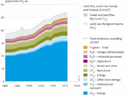
Figure 2.1 describes the main sources of the different GHG, under this topic the sources involved would be emissions from “Waste and other”, “Agriculture” and “Forest and peat fires”.
Figure 2.1 Global GHG emissions, per type of gas and source, including LULUCF. Source: Edgar v.4.3.2
(EC-JRC/PBL, 2017)
Atmospheric CH4 concentrations increased by approximately 150% beyond the pre-industrial
level (IPCC, 2007) reaching 1834 ppb in 2015 (Reay et al., 2018); with an estimated contribution of approximately 70% attributed to biogenic sources (Conrad, 2009): wetlands, landfills and livestock production. Nevertheless, a large fraction of CH4 produced is rapidly
consumed by microorganisms before it enters the atmosphere (Frenzel, 2000; Reeburgh, 2003), specially during aerobic methane oxidation (methanotrophy) as regarded in Figure 2.2:
5 Figure 2.2 Methane oxidation rate of methanotrophs from different ecosystems (Forest Soil, Leafy Compost, Riverbed Soil, Wetland Soil, Dumpsite Soil and Rice Field Soil, respectively). Source: Brindha and Vasudevan, 2017 N inputs to the ecosystems are also increasing with human activities. During the first decade of the twentieth century, the worldwide demand for N-based fertilizers far exceeded the existent supply. It was only in 1912 when the first commercial plant produced industrially synthetized ammonia (NH3) via the Haber-Bosch process to meet the needs of the growing
world population, which has subsequently increased globally by 78% since 1970 due to a rapidly increasing population, and led to an increase of anthropogenic reactive nitrogen (Nr) in the environment by 120% (Galloway et al., 2008). Agricultural demand for nitrogen fertilizers’ application, livestock production and land use changes are considered to be the main sources of Nr pollution. The “nitrogen use efficiency” (NUE) in crop production is considered to be less than 50% in most farm productions in the world (Lassaletta et al., 2014) and the actual fraction emitted by the nitrogen-based fertilizers is still uncertain (Davidson, 2009) considering the wide range of environmental external variables and the different applied agricultural techniques. Crop residues were reported to be highly correlated with N2O emissions rather than inputs of
N from manure/fertilizer (Pugesgaard et al., 2016), although more investigation is needed for residue composition and quantity analysis (Baggs et al., 2003). Moreover, not only the quantification rates of N2O are difficult to determine but its spatial and temporal variation
6
2.2 Garden waste policy and management
Garden waste in EU Waste Frame Directive 2008/98/EC is inserted in the bio-waste definition “biodegradable garden and park waste, food and kitchen waste from households, restaurants, catering and retail premises and comparable waste from food processing plants”. The lack of separation of bio-waste makes it practically impossible to directly measure the mass of garden waste generated as there would be a need for collection, sorting, processing and transport from the source until the treatment/recycling facilities.
The actual fraction of bio-wastes from Municipal Solid Waste (MSW) classified as recycled by the EU are the amounts reported to Eurostat as the digested or composted material (EEA, 2013) as shown in Figure 2.3. where Portugal recycled around 13% and UK 17% with the difference of bio-waste collection at the households.
Figure 2.3 Composting and digestion rate of municipal waste in 2013 together with the municipal states who apply a door to door collection of biowaste (EUROSTAT, 2019)
7 In order to transition to an efficient circular and green economy, generated waste needs to be minimised at a variety of scales from a wide range of sources. For this particular waste, its decline in production indicates a reduction of green areas. As the main idea is to have an increase of green spaces specially in urban areas, it is important to understand how to profit the most from it. In this sense it is important to prioritize and develop actions which can be applied to achieve these goals.
As population tends to grow so does the waste production and reducing its GHG emissions will become more complicated. A good solution is to lead the emissions into a positive GHG flux balance, in other words, to benefit from the emitted gases in a controlled manner instead of ending in a landfill. Thereby, a number of treatments and pre-treatments is performed, with different efficiencies:
Mechanical-Biological Treatment (MBT)
MBT is a complement to other further treatments, works as a pre-treatment where it sorts biodegradable and non-biodegradable waste from a mixed waste stream and then applies a biological treatment to address the waste into a next suitable treatment (UK Governament, 2013).
Anaerobic Digestion
Anaerobic digestion of bio-waste can be advantageous considering the CH4 and CO2
emissions from the biodegradation to produce biogas and replace the use of fossil-fuels. After digestion, the digestate goes through a posttreatment to filter the liquid and separate the solids. This solid fraction, after stabilization, can be directly used as an organic amendment or compost (Fruteau de Laclos et al., 1997). The methane yield will be highly dependent on the waste composition, considering bio-waste being the “vegetable-garden-fruit” (VGF) fraction of the MSW the garden waste may hinder the process because of its lignocellulosic content requiring always a pre-treatment.
8 Composting
Composting involves the microbial oxidation of OM turning the waste into a humus-like material. This activity is also becoming a solution for garden waste in Europe, allowing to partially replace fertilizers or peat compost, thus avoiding the associated emissions of GHG from the fertilizers and the damage made to peatlands ecosystem. Although the GHG emission from composting in open vessels (windrow composting) is still a disadvantage (Andersen et
al., 2010), which is the case for several member states of Europe, at a smaller scale is also
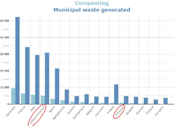
done for households. Contrary in the compost heat recovery systems (CHRS) (closed reactors) producing compost and recover energy at the same time for on-site purposes, helps to diminish the GHG flux about -10 kg CO2 eq/tonne of the MSW (Smith et al., 2001). Figure 2.4 shows
how much of the MSW ends as a compost: UK, having a surface almost 3 times higher than Portugal, produced 6 times more waste than Portugal in 2017 having 16% of it ending in compost while Portugal composted 20% of the total MSW generated.
Figure 2.4 Compost production and MSW generation based on OECD data from 2017. Units: Tonnes, Thousands.
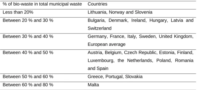
9 Even though Portugal had a higher percentage of composted material, it is important to understand the actual fraction of biowaste in the MSW, and in the following table (Table 2.1), which gives an idea of the amount of bio-waste which can be found in the MSW in European countries, it is possible to see the higher potential for compost that Portugal has in respect to UK. Keeping in consideration that this table is based on 2008 to 2010 data, the tendency for generated waste per capita has been slightly decreasing: from 2011 to 2017 Portugal and UK produced, respectively, -0.6 % and -4.68 % kg (EUROSTAT, 2019).
Table 2.1 - Bio-waste share in municipal waste in 28 European countries in 2008–2010. Source: (EEA, 2013)
% of bio-waste in total municipal waste Countries
Less than 20% Lithuania, Norway and Slovenia
Between 20 % and 30 % Bulgaria, Denmark, Ireland, Hungary, Latvia and Switzerland
Between 30 % and 40 % Germany, France, Italy, Sweden, United Kingdom, European average
Between 40 % and 50 % Austria, Belgium, Czech Republic, Estonia, Finland, Luxembourg, the Netherlands, Poland, Romania and Spain
Between 50 % and 60 % Greece, Portugal, Slovakia Between 60 % and 80 % Malta
The application of organic amendments, like the green waste compost, the digestate from anaerobic digestion, or even applying directly green waste on top of soils (mulching), are practices with positive impacts when it comes to preventing soil erosion, increasing moisture conservation and fertilisation effects (Mulumba and Lal, 2008). Favourable effects of residue mulching on soil organic carbon (SOC), soil water retention and percent water-stable aggregates have been reported for the surface layer (Duiker and Lal, 1999). Mulching the top soil will also prevent runoffs, loss of moisture content of the soil, can be a protection for seedlings and other benefits (Rathore et al., 1998). However, the actual GHG emissions from decaying matter, particularly during composting process, are recognized for being considerable but not well quantified (Baggs et al., 2003; Dalal et al., 2008; Skiba et al., 2012; Verdi et al., 2018).
10 Biowaste and GHG
As aforementioned, green waste belongs by definition in the biowaste section. Its evaluation and statistical analysis in municipalities it is still scarce as a result of its poor valorisation as a waste. As so, in this section the data its related to all the waste integrated in the biowaste definition.
In section 2.2, discussing treatments for MSW management, landfill wasn’t stated as one of the options because of its noxious consequences. Biowaste in landfills increasesGHG emissions as a result of its biodegradation, Table 2.2 indicates CH4 as a major constituent from
the gas composition from landfills. Concurrently, Figure 2.5 shows the associated GHG emissions in CO2 eq. from landfill, among others, throughout the years in the UK.
Table 2.2 Composition of landfill gas. Source: Themelis and Ulloa, 2007
Composition of landfill gas
Compound Average concentration (%)
Methane (CH4) 50
Carbon dioxide (CO2) 45
Nitrogen (N2) 5
Hydrogen sulphide (H2S) < 1
Non-methane organic compounds (NMOC) 2700 ppmv
In 2016 in the UK, 4% of the GHG emissions mainly comprising methane, came from the decomposition of biodegradable waste in landfill sites (CCC, 2018). In the same year in Scotland, 1.15 Mt of biowaste went to landfill (Zero Waste Scotland, 2019), even though its reduction has been considerable as regarded in Figure 2.5.
11 Figure 2.5 GHG emissions from waste by source in UK (1990-2016). Source: (CCC, 2018)
In Portugal the waste sector, including waste water, is responsible for the 9.6% of the national GHG emissions (PERSU, 2016). The lack of separate collection of biowaste in Portugal leads to its deposition in a landfill incrementing its GHG emissions.
Figure 2.6 MSW and bio-waste in landfills in Portugal. Source: Fernandes et al., 2018.
In table 2.1, about 50% of the MSW in Portugal is biowaste and together with figure 2.6 suggests that 50% of the biowaste produced ended in a landfill. Even so, the amount of biowaste produced is highly uncertain when there’s no separate collection of this type of waste.
12
2.3 Nitrous Oxide (N
2O)
Soils are the largest source of natural and anthropogenic N2O. Although agricultural soils are
considered the most significant source of anthropogenic N2O emissions due to fertiliser
application, non-agricultural soils are gaining importance as disturbance of natural N cycles becomes more apparent in the environment. N2O impacts, as mentioned in the succeeding
chapters, are highly variable and unpredictable in both terrestrial and aquatic systems (Gruber and Galloway, 2008).
It should be emphasized that the largest loss of nitrogen from terrestrial soils tends to be through ammonia (NH3) volatilisation and production of inert dinitrogen (N2) via denitrification.
However, NH3 emissions are typically a result of high N concentrations in the soil (i.e. fertiliser
events and deposition of animal waste) and warm weather, while N2 is the final product of
denitrification, limited in some instances due to the lack of the N2O reductase enzyme in
bacteria resulting in N2O as the final product.
Garden waste composition is an important factor to be analysed because of the available N which can be provided to the soil and its consequential N-loss through gas emissions. The N content varies from season to season as described in Figure 2.7 where N content is highest during summer and autumn months corresponding to when grass clippings or leaves are the major constituents.
Figure 2.7 Seasonal variation in carbon and nitrogen content, and C/N ratio of garden waste in Netherlands (Boldrin and Christensen, 2010). Please note different scales for y-axis.
13 Thus, the N-gas focused in this study will be N2O due to its GWP and related impacts discussed
in section 2.4.
2.4 Nitrogen net sink
Nitrogen pollution is predominantly diffuse pollution, lacking of a specific point of discharge. Its loss can be under different forms: gaseous, leachate and particles deposition either wet or dry; largely due to mechanisms like soil erosion, leaching, ammonia volatilization, ammonia oxidation and denitrification (Thomson et al., 2012).
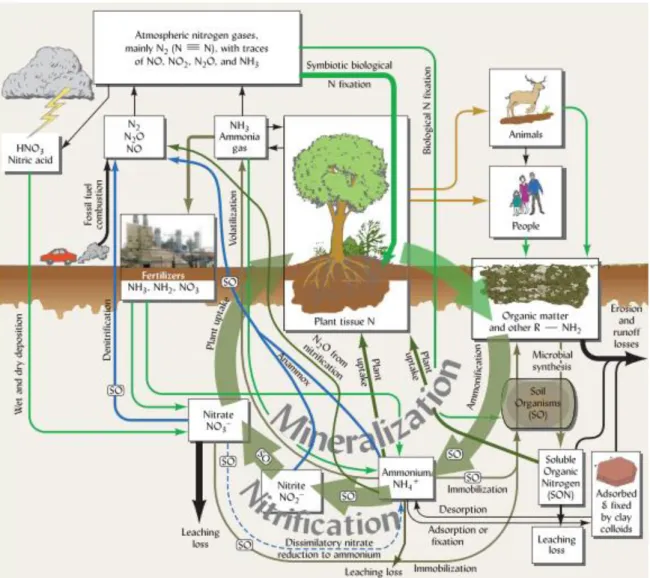
Figure 2.8 This figures shows N complexity through its many valence states and phases (gas, liquid, and solid). The arrows represent processes by which one form is transformed into another. Note the processes by which nitrogen is lost from the soil and by which it is replenished (bright green arrows). The blue arrows represent anaerobic processes. Soil organisms, whose enzymes drive most of the reactions in the cycle, are represented as rounded boxes labeled “SO.” (Weil and Brady, 2016)
Agriculture land is an important source of diffuse pollution, accounting for about 50% of all the ammonia that is volatilised worldwide (Sommer et al., 2004).
14 Besides agriculture, natural land also contributes largely to global N2O emissions (6 Tg N yr-1)
(Thomson et al., 2012). Altogether, the soil contributes approximately 57% to the total annual global emission (IPCC, 2006c).
The N gas emissions (NH3, N2O, NOx) can have detrimental implications such as acid rains
and increasing the ozone in the tropospheric layer and damaging the stratosphere. In the lower atmosphere N2O it is a relatively inert gas but in the stratosphere it is broken down by UV light,
producing oxygen radicals and thus ozone (O3), which filters out ultraviolet radiation from the
sun. Ozone in the troposphere acts like a GHG, damages the plants and is bad for human health (Ramanathan et al., 1985).
Organic wastes, whether applied to agricultural soils or left behind, are a source of nutrients (such as N and phosphorus (P)) for plant uptake. However, a large fraction of it is not readily available, and stays in pools interconnected by several possible mechanisms regulated by the environmental conditions. Nutrients can be lost to the atmosphere as beforementioned, leached or be assimilated in the OM, preventing plant uptake.
N when leached (predominantly under as NO3-), can cause several effects on waterbodies
and soil’s productivity. N leaching, together with other macronutrients transported into waterbodies may cause eutrophication. It has been shown that poor management of organic wastes(such as garden wastes and manure) can cause algal blooms and the consequent decline of aquatic ecosystems if washed into drainage systems during storms via decreasing oxygen availability (Strynchuk, et al., 1999; Smith and Schindler, 2009).
Both NH4+ and NO3- can also cause acidification of the soil in different ways: NH4+ can decline
soil buffer capacity by displacing base cations (Na+, Ca+, K+, Mg2+) and once is consumed by
root systems it releases H+ into the soil. NO
3- has a tendency to leach and with it basic cations
and metal cations, causing mobilisation of Aluminium (Al) (Gundersen et al., 2006; Tian and Niu, 2015).
The nitrogen cascade (Figure 2.8) involves the cycling of N amongst the different natural compartments such as air, soil, living organisms and water. The following subchapters will focus on the main N pathways in the different natural compartments present in the study.
Soil N balance
Nitrogen budgets seek to summarize the complex agricultural N cycle by documenting the major flow paths of N in various dynamic N pools, based on the principle of mass conservation (Eq. 2.1) (Meisinger et al., 2008):
15 Meisinger (1984) made the division between systems for N balances based on “whole crop” vs. the “aboveground crop” approach.
Nitrogen can be found in soils in different forms of biomass such as in soil organisms and microorganism, or trapped in organic matter and/or clay substrates under organic and inorganic forms (Cameron et al., 2012).
N – Fixation
N-Fixation is the conversion of atmospheric N (N2) to a form of reactive nitrogen in the
biosphere. This process happens in nature through biological nitrogen fixation; but the primary anthropogenic route is through the synthetic chemical Haber Bosch process.
• Chemical (Haber Bosch)
The industrial process that produces ammonia (NH3) from molecular hydrogen (H2) and
molecular nitrogen (N2) under high pressures and temperatures (20 MPa and 500°C) with a
contribution of, approximately, 3% of the global emissions of CO2 (Smith et al., 2012; Cai et
al., 2017).
• Biological Nitrogen Fixation (BNF)
Several natural agents carry out this biological process, including actinomycetes in forest ecosystems, cyanobacteria in wetlands and rhizobacteria in grasslands and agricultural soils in symbiosis with Fabaceae (Weil and Brady, 2016).
Soil moisture is an important factor for N-fixation, as there needs to be sufficient water in the soil to activate cyanobacterium activity. However, over hydration may lead to depletion of energy reserves necessary for N fixation. Where moisture content fluctuates between wet and dry, the N-fixation rates in soils can increase (Belnap, 2001). The temperature is also vital for microorganism activity, the optimum for N-fixation is 20–30 °C but activity has been observed between –5 and 30 °C (Belnap, 2001).
The optimal pH for N-fixation and microorganisms activity is approximately 7 and above (Davey and Marchant, 1983; Hungria and Vargas, 2000), yet if the pH is above 8 there’s a depression in microbial activity (Granhall, 1970)
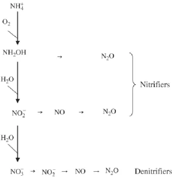
Nitrification
Norton and Stark (2010) describe nitrification as a biological conversion of reduced nitrogen (N) in the form of ammonia (NH3) or ammonium (NH4+) or organic N to oxidized N in the form
16 The conversion of N from a cation to an anion state may improve plant uptake in some cases (Tang and Rengel, 2003), although both forms are available for the plants the anion is more mobile in soils due to its capacity to not get adsorbed in the soil matrix (Varennes, 2003). Nitrification can be described in two steps (Arp and Stein, 2003) where the key element are the ammonia oxidizing bacteria (AOB), also described as chemolithotrophs because they can derive all their energy for growth from the oxidation of the ammonia to nitrite (Arp, 2009). The first step result, carried out by the Nitrosomonas bacteria, is hydroxylamine (NH2OH)
which is then catalysed by hydroxylamine oxidoreductase (HAO) converting NH2OH into nitrite.
The nitrite ion is then oxidized by Nitrite oxidizing bacteria, like Nitribacter and converted into nitrate ions completing the nitrification process (Varennes, 2003) as presents in Eq. 2.2:
NH4+ → NH2OH → NO2− → NO3− [2.2]
This last procedure is carried out by autotrophic bacteria but some heterotrophic bacteria (and also fungi) can carry out parts of the process, more commonly designed as heterotrophic nitrifiers (Prosser et al., 2007). These rates are typically lower because they cannot obtain energy from the oxidation of the organic and inorganic forms of N.
The nitrification process produces nitrogenous gaseous losses as a by-product from the microbial activity. N2O produced at a global level from nitrification processes has a significant
impact over the greenhouse effect and the ozone layer (Hutchinson and Davidson, 1993; Gödde and Conrad, 2000). The gases produced by the AOB are NO, N2O and NO2, which can
17 For nitrifying bacteria the optimum soil temperature and pH is between 25-30ºC and 4.5-7.5 respectively (Haynes, 1986).
It is demonstrated that nitrification rates increase up until 60% water filled pore space (WFPS) which is most soils field capacity (Davidson and Verchot, 2000).
N-Volatilization
N-volatilization consists on gaseous nitrogen form NH3 lost from the soil top layer into the
atmosphere (Mattos et al., 2003) as shown in Eq. 2.3.
NH4+ + OH⎯→NH3 + H2O [2.3]
At a high pH, soils tend to lose a significant amount of ammonia especially when temperatures are higher (25-30 ºC) (Sommer et al., 2004), although neutral or acid pH soils can also lose NH3 if urea is applied due to its high concentrations (Black et al., 1985).
The amount of emitted ammonia is related to the ammonium concentration found in the soil, consequently is related to rates of different processes which influence the soil N-balance (N-uptake, nitrification, denitrification…) (Black et al., 1985; Cameron et al. , 2012).
Kravchenko et al. (2002) showed that soil cation-exchange capacity (CEC) has a big influence on the NH4+ mobility, the higher the soil CEC the lower its mobility, thus affecting NH3
volatilization.
18 Denitrification
Denitrification is most active under anaerobic conditions where there are high concentrations of both oxidised nitrogen compounds (NO3- , NO2-) acting as terminal electron acceptors in the
absence of oxygen, to be reduced into gaseous oxides (NO, N2O), which may themselves be
further reduced to dinitrogen (N2). NO3- can also be reduced to NH4+ via NO2-, with N2O being
produced, this process is designated as nitrate ammonification and can take place in the same environmental conditions as denitrification (Eq. 2.4) (Canfield, Kristensen and Thamdrup., 2005; Thomson et al., 2012).
NO2−
𝐴𝑚𝑚𝑜𝑛𝑖𝑓𝑖𝑐𝑎𝑡𝑖𝑜𝑛
→ NH4
NO2− ⎯→ NO ⎯→ N2O ⎯→ N2
As well as biological denitrification described above, there’s also the chemical denitrification or chemo denitrification based on the reduction of nitrite ions, which are unstable in acidic environments, through oxidation of organic N by NO2- with N2 gas as output (Christianson and
Cho, 1983).
Soil moisture fluctuation influences the denitrification through the aeration of the soil, meaning if the soil moisture is higher than the field capacity the denitrification rates will increase due to the anoxic conditions developed; contrarily to nitrification, above 60% WFPS denitrification is the predominant process in the production of N2O emissions (Müller and Sherlock, 2004).
The addition of organic C compounds to the soil eases the complete denitrification process inducing anaerobiosis through stimulation of O2 demand, reducing emissions of N2O and NO
and emitting directly N2 (Vallejo et al., 2004).
Anammox
Anammox stands for anaerobic ammonium oxidation and in this case ammonium and nitrite are biologically converted, directly, to N2 and N2O gas; N2O can be inhibited by nitrite presence
(Strous et al., 1999; Thomson et al., 2012)
Anammox is inhibited by the presence of nitrite, higher than 0.1 g per litre (Strous et al., 1999). Strous et al. in 1998 developed the stoichiometry based on the mass balance (Eq.2.5):
19 𝑁𝐻4++ 1.32𝑁𝑂2−+ 0.066𝐻𝐶𝑂3−+ 0.13𝐻+
→ 0.066𝐶𝐻2𝑂0.5𝑁0.15+1.02𝑁2+ 0.26𝑁𝑂3−+
2.03𝐻2𝑂 [2.5]
N- MIT (Mineralization-Immobilization Turnover)
Mineralisation occurs during organic matter decomposition. Microorganisms use complex organic compounds as a source of energy and transform them into smaller more readily available compounds ( Jansson and Persson, 1982).
N mineralization divides into three processes carried out by heterotrophic microorganisms and autotrophic bacteria focused on the nitrification. The heterotrophic perform the aminization, transforming the complex nitrogenous organic compounds into simpler ones like amines, which then are used to be turned into ammoniated compounds through the ammonification (Eq. 2.6) (Tisdale and Nelson, 1985; Rodrigues and Coutinho, 2000):
NH3+ H20 ⎯→ NH4+ OH± [2.6]
But immobilization can occur when the products from mineralization are reused by microorganisms, integrating the compounds in its tissues or in non-cellular organic matter (humus) making nitrogen unavailable for plant uptake.
Mineralization and immobilization can happen at the same time, reason why is referred as Mineralization-Immobilization Turnover (MIT).
Tisdale (1958) indicates the different C/N values to determine MIT. C/N between 20:1 and 30:1 is the perfect ratio for an efficient plant N uptake. For residues with high rates of C/N applied to the soil, as shown in the first plot from Figure 2.10, there is an immobilization of mineral N because of the N content consumed by microbial activity, leading to the depletion of the soluble N in the soil and consequently creating a nitrate depression period affecting the possible plant uptake. The underneath plot describes what happens when the residues have a low rate of C/N, meaning there is more N content than necessary, therefore the soluble N content in the soil increases.
20 Plant uptake
Inorganic N is preferred for plant uptake, typically in the form of NH4+ and/or oxidized NO3
-rather than other dissolved organic N (DON) forms (e.g., urea, amines, proteins, and nucleic acids) which are absorbed in smaller quantities or are mineralized into inorganic forms by microorganisms (Nacry et al, 2013). Although van Breemen (2002) suggested that more investigation is needed in DON plant uptake specially in N-limiting environments. The referred inorganic forms are very dynamic, and can be consumed as fast as they are produced, especially in well aerated soils with neutral pH (Jones et al., 2004).
Soil-Water
The soil-water content and water filled pore space (WFPS) of soils influences the ratios of N2O:NO:N2 emissions as demonstrated in the hole-in-the-pipe (HIP) model (Davidson and
Verchot, 2000). Moving water can work as a transport of oxygen throughout the soil system, it also has the important part of transporting NO, N2O and N2 out of the soil.
Figure 2.10 Mineralization-Immobilization turnover explained by residues added with different C/N ratio. Source: Weil and Brady, 2016
21 Generally conditions can be summarised into three situations: a dry well aerated soil, where oxidative process is predominant, with NO production higher than N2O or N2; a wet soil with
poorly aerated soil thus the most reductive oxide is the dominant product, N2O; and a very wet
soil that creates anaerobic conditions so nitrogen oxide forms are consumed by the nitrifiers, releasing mostly N2 as a result (Davidson and Verchot, 2000). Due to the heterogeneous
nature of soil, all of these processes can occur in tandem in macrosites within the soil structure, making identification of the dominating process at any given location difficult and highly spatially variable.
N-Leaching
NO3- leaching is directly related to the concentration of N in the soil, and consequently the rates
of nitrification-denitrification, which in turn is dependent on soil moisture and rainfall/irrigation that regulates the soil aeration being this essential for nitrification rates.
NO3- leaching will also depend on temperature, as lower temperatures reduce production of
NO3- (Russell et al., 2007). Soil type is also important, as if it is a poorly structured sandy soil
there’ll be more macropores helping on the aeration of soils and consequently decreasing denitrification rates and facilitating the water movement which increases NO3- leaching
(Cameron et al. , 2012). On the other hand, clay soils can fix N in their small pores, reducing leaching but also reducing accessibility to microorganisms.
2.5 Methane (CH
4)
Methane is a heat trapping gas with the most abundant reactive trace gas in the atmosphere and its sources can be either natural or anthropogenic. The natural sources considered significant are the oceans, termites’ activity and wetlands. Wetlands are the main natural source of CH4, with an emission of 177 and 284 Tg year−1 (Reay et al., 2018) but its high
diversity (swamps, bogs, forest floods, etc) and spatial variability makes the CH4 emission
evaluation a challenge. A novel source has been also reported, Keppler et al. (2006) estimated an CH4 emission of 1–7 Tg yr-1 for plant litter under aerobic conditions suggesting that sunlight
has a significant influence on the methanogenesis (Bloom et al., 2010). Nevertheless, bio-waste can have a substantial impact in CH4 emissions as it can be regarded in the following
figure (Figure 2.11) in “Residential (biomass)” together with the other 11 top anthropogenic global sources of methane.
22 Figure 2.11 Global CH4 emissions by source in 2016 presented in megatonnes of CO2 equivalent. Source:.
(CCC,2018)
2.6 Methane net sink
The main sinks for CH4 emitted into the atmosphere can be divided in three categories:
Non biological oxidation of CH4 by UV-created hydroxyl (OH) radicals in the troposphere is the
most important sink, destroying circa 90% of the CH4 present in the atmosphere (with a
concentration of approximately 1.7 ppm) (Smith et al., 2003). Secondly, is stratospheric chemical reactions, which is less dense and not as vertically mixed by convection. These characteristics will allow CH4 to enter from below and being consumed by chemical reactions,
with OH radicals in the lower stratosphere and by reaction with chlorine radicals or oxygen atoms in the upper stratosphere (Jardine et al., 2004).
The third main sink for atmospheric CH4 removal takes place in the ground-atmosphere
interface, where about 6% is oxidised and consumed by microorganisms in aerobic soils (Dalal
et al., 2008).
The balance of methane in the soil dwells between what is consumed by oxidation (methanotrophy) and what is emitted in anaerobic conditions (methanogenesis), if the activity of methanotrophic bacteria and methanogenic bacteria is positive it works as a source of emission (Le Mer and Roger, 2007)
Watanabe et al.(2007) stated that the majority of methane produced is biologically from anaerobic decompositions under anoxic conditions with very low redox potential, carried out by methanogenic archaea. A good example of these environments would be the lakes and the wetlands.
23 Figure 2.12 Soil methane cycle based on Loïc Nazaries et al (2013)
Methanogenesis
Methanogenesis occurs in anaerobic conditions by methanogenic bacteria doing anaerobic digestion of organic matter, these are decisive factors for CH4 production (Dalal et al., 2008).
Methanogens produce methane as metabolite in energy production through two different pathways (Lai, 2009):
CH3COOH → CH4 + CO2 [2.7]
(Acetotrophic methanogens)
4H2 + CO2 → CH4 + 2H2O [2.8]
(Hydrogenotrophic methanogens)
Although methanogenesis takes place under anaerobic conditions, there are some studies showing that is imprudent to discard the hypothesis of CH4 formation under aerobic conditions
24 Methanotrophy
Methanotrophic bacteria can be found in well-aerated surface soils and oxidize CH4 to
generate energy and fix CO2 into organic compounds, contributing up to 10% of global CH4
oxidation (Smith et al., 2003; Lowe, 2006) but biological CH4 oxidation is also done by
anaerobic archaea in association with anaerobic bacteria. In mesophilic anaerobic conditions, NO2- can work as an inhibitor for the methane oxidation, consisting in a mechanism of
nitrite-dependent anaerobic oxidation of methane theory (Ettwig et al., 2010). The following equation [2.9] is adapted from Ettwig et al., 2010:
3CH4 + 8NO2−+ 8H+= 3CO2 + 4N2+ 10 H2O [2.9]
(∆𝐺°’ = −928 𝑘𝐽 𝑚𝑜𝑙 − 1𝐶𝐻4)
There are also references concluding that NH4+ has a strong influence as an inhibitor of
atmospheric CH4 oxidation, which can suppress soil CH4 consumption by up to 70% (Boeckx
25
3 Materials and methods
This experiment was carried out in two locations; a) Easter Bush, Midlothian (UK) (55°51'50.1"N 3°12'44.0"W) in 2017 and b) Lisbon Portugal (38°42'50.8"N 9°11'12.4"W) 2017/18. To quantify the GHG emissions from garden waste materials at a home-scale, several measurements were carried out in boxes/pots with different treatments established outdoors.
3.1 Site description
Edinburgh, Scotland, has a temperate hyperoceanic climate characterized by cold winters with an average temperature of 4 °C and cool summers with an average temperature of 14 °C, and its average annual precipitation is 920 mm, evenly distributed.
Lisbon, Portugal, has Mediterranean climate characterized by cold wet winters with an average temperature of 11 °C and dry hot summers with an average temperature of 23 °C, and an annual precipitation of approximately 800 mm (IPMA, 2019).
Figure 3.1 Air and soil temperature (°C) and precipitation (mm), for Portugal from November 2017 to May 2018 (left) and Scotland from January to December 2017 (right) based on data from meteorological stations during experiment..
In order to ensure that the samples reflect local microbial activity, measurements took place between April and August of 2017 (122 days) in Scotland, and between November and May of 2017/18 (167 days) in Portugal, to reflect the peak from growths season.
The substrates for the experiment were collected from both sites using the same experimental approach. In Scotland, the sample was taken from a grassland with Eutric Cambisol. The soil in Lisbon is a Haplic Vertisol with loamy clay texture (FAO, 1998).
26 Table 3.1 - Soil type and grass species properties measured from Portugal (November, 2017) and Scotland (May, 2017).
Parameters Lisbon, ISA Edinburgh, CEH
Soil Haplic Vertisol Eutric Cambisol
pH 7.6 6.5
C:N 19.73 11.72
Grass Panicum Repens L. Lolium Perenne L.
MC (%) 1 60.25 79.03
N content (%) 1.83 2.57
C content (%) 86.10 61.75
2: Moisture Content
3.2 Field experiment
Both systems were set up outdoors throughout the study.
Three different treatments were applied in both sites: a control treatment with a soil layer (S), a second treatment with the same substrate layer plus covered by garden waste (S+GW) and a third treatment with only garden waste decomposing and no soil (GW).
In Scotland, the systems were assembled in transparent plastic boxes (78 x 56 x 43 cm), each box composed by a gravel layer to improve water drainage, topped with a layer of filtering textile and then covered with the respective treatment. This system was composed by 3 replicates for each treatment.
27 In Portugal, the same methodology was applied with different materials. Kick-Brauckmann-pots (25.5 x 28 Ø cm) were used rather than boxes to also facilitate the water flux, thereby disregarding the need for a gravel layer. This system, because of the smaller area available per pot, was composed by 5 replicates for each treatment to provide a better estimate of the spatial variability.
Figure 3.3 Kick-Brauckmann-pots assembled in Portugal for the different treatments
Figure 3.2 Boxes assembled in Scotland for treatment with soil and garden waste (left) and with soil and no garden waste (right)
28 Table 3.2 Outline of the assembled systems for each treatment for Scotland and Portugal with the respective applied garden waste. *Available volume for measurements
Site Treatments Replicas V (m3)* Garden
Waste (Kg) Scotland S 3 0.036 0 S+GW 3 0.036 1 GW 3 0.053 1.2 Portugal S 5 0.017 0 S+GW 5 0.017 0.1 GW 5 0.017 0.4
3.3 Measurements
Flux measurementsGaseous flux measurements were carried out once or twice a week, depending on the meteorological events, through a static gas chamber methodology (Hutchinson and Mosier, 1981) followed by a gas chromatography lab analysis.
29 In Scotland, the boxes were sealed with a lid, containing neoprene sponge attached to the underside, and a fan to improve air mixture. The lid was closed with clips for a better sealing system. In Portugal the sealing was achieved with a plastic lid. All chambers were sealed during 60 min to obtain a concentration gradient for the GHG flux. Four samples were collected from each plot through a 100 mL syringe at t = 0, 20, 40 and 60 min and flushed into a 20 mL glass vials using 2 needles so air could flow through by pressure, flushing the vial with 500 % of its volume.
The samples were then analysed using a Hewlett Packard 5890 series II gas chromatograph (Agilent Technologies, Stockport, fitted with an electron capture detector). The GC can have associated errors when it comes to the calibration curve and with sample concentration values close to the limit can result in anomalous values. Four sets of four calibration standards were used per GC run of 108 samples to improve quality control.
The concentration rate of gas flux from the soil was calculated according to Eq. 3.1:
𝐹 = 𝑑𝐶
𝑑𝑡0 ×
𝜌𝑉
𝐴 [3.1]
Where F is the gas flux emitted from the soil (μmol.m-2.s-1), dC is the change in concentration
in mol.mol-1, dt the change in time in s, ρ the air density in mol.m-3, V the chamber volume in
m3, and A the surface available in the chamber for measurement in m2.
Fig. 5 - sealed boxes for measurements and vials for gas measurements Figure 3.5 Sealed boxes ready for mensuration and the vials to collect the gas samples