A Probabilistic Framework for Automatic
and Dependable Adaptation in Dynamic
Environments
Mônica Dixit, António Casimiro, Paulo Verissimo
Paolo Lollini, Andrea Bondavalli
DI–FCUL
TR–2009–19
January 21, 2010
Departamento de Informática
Faculdade de Ciências da Universidade de Lisboa
Campo Grande, 1749–016 Lisboa
Portugal
Technical reports are available at http://www.di.fc.ul.pt/tech-reports. The files are stored in PDF, with the report number as filename. Alternatively, reports are available by post from the above address.
A Probabilistic Framework for Automatic and
Dependable Adaptation in Dynamic Environments
Mônica Dixit, António Casimiro and Paulo Verissimo∗
University of Lisboa
Paolo Lollini and Andrea Bondavalli†
University of Firenze January 21, 2010
Abstract
Distributed protocols executing in uncertain environments, like the Inter-net, had better adapt dynamically to environment changes in order to preserve QoS. In earlier work, it was shown that QoS adaptation should be depend-able, if correctness of protocol properties is to be maintained. More recently, some ideas concerning specific strategies and methodologies for improving QoS adaptation have been proposed. In this paper we describe a complete framework for dependable QoS adaptation. We assume that during its life-time, a system alternates periods where its temporal behavior is well charac-terized, with transition periods during which a variation of the environment conditions occurs. Our method is based on the following: if the environ-ment is generically characterized in analytical terms, and we can detect the alternation of these stable and transient phases, we can improve the effec-tiveness and dependability of QoS adaptation. To prove our point we provide detailed evaluation results of the proposed solutions. Our evaluation is based on synthetic data flows generated from probabilistic distributions, as well as on real data traces collected in various Internet-based environments. Our results show that the proposed strategies can indeed be effective, allowing protocols to adapt to the available QoS in a dependable way.
1 Introduction
Computer systems and applications are becoming increasingly distributed and we assist to the pervasiveness and ubiquity of computing devices. This openness and complexity means that the environment (including network and computational plat-forms) tends to be unpredictable, essentially asynchronous, making it impractical,
∗University of Lisboa, Portugal. E-mails: mdixit@di.fc.ul.pt, casim@di.fc.ul.pt, pjv@di.fc.ul.pt. †University of Firenze, Italy. E-mails: lollini@dsi.unifi.it, bondavalli@unifi.it.
or even incorrect, to rely on time-related bounds. On the other hand, in several ap-plication domains (e.g. home and factory automation, interactive services over the internet, vehicular applications) there are strong requirements for timely operation and increased concerns with dependability assurance. Although strict real-time guarantees cannot be given in such settings, one possible way to cope with the uncertain timeliness of the environment while meeting dependability constraints, consists in ensuring that applications adapt to the available resources, and do that in a dependable way, that is, based on some exact measure of the state of the
en-vironment. Dependability will no longer be about securing some fixed temporal
bounds, but about using the correct bounds at any given time.
In this paper we build on earlier work that introduced the necessary archi-tectural and functional principles for dependable adaptation [6]. In essence, the idea behind dependable adaptation is to ensure that assumed bounds for funda-mental variables are adapted throughout the execution and always secured with a known and constant probability. For instance, consider an application that defines a timeout value based on the assumed message round-trip delay. This application will adapt the timeout during the execution with the objective of ensuring that the probability of receiving timely messages will stay close to some predefined value. Therefore, when message delays increase or decrease, the timeout will also in-crease or dein-crease in the exact measure of what is needed to ensure the desired stability of the probability value. In other words, this application will secure a
coverage stability property.
Clearly, this is only possible if some limits are assumed on how the environ-ment behaves. For instance, if message delays can vary in some arbitrary fashion, then any observation or characterization of the environment will be useless, in the sense that nothing can be inferred with respect to the future behavior. Fortunately, this is not the usual case. There may be instantaneous or short-term variations that are unpredictable and impossible to characterize, but medium to long-term varia-tions typically follow some pattern, allowing to probabilistically characterize the current operational state and derive the bounds that must be used for achieving coverage stability.
A baseline approach, which was introduced in [6], is to make very weak as-sumptions about the environment— just that it behaves stochastically, but with unknown distributions. This weak model was nevertheless sufficient to illustrate the concept of dependable adaptation.
More recently, in [5], we introduced a new approach based on different assump-tions about the environment behavior and we conducted some initial experiments to observe the potential improvements with respect to the original, and pessimistic, approach.
In this paper we provide a complete and detailed description of our work, in-cluding an extensive set of experimental results that we use to thoroughly evaluate and quantify the benefits of the proposed approach and of the implemented mech-anisms.
stochas-tic behavior is well characterized, with transition periods where a variation of the environment conditions occurs. Because of that, we are able to move away from conservative (and pessimistic) solutions, with possibly little relevance in practice, to more reasonable ones, which have interesting practical reach. We introduce a framework that is based on the use of statistical formulations for the recognition and characterization of the “state” of the environment. The framework includes phase detection mechanisms, based on statistical goodness-of-fit tests, to perceive the stability of the environment behavior. Additional mechanisms to derive the ac-tual parameters of the distributions are also employed. The paper explains how the chosen methods were implemented, which is relevant to show how dependability constraints are handled in practice.
A fundamental aspect of our work is that we are concerned with dependability objectives. Therefore, our main contribution is the provision of a framework that takes as input dependability-related criteria (the required coverage of an assump-tion) and supports adaptation processes by providing information on how adapta-tion should be done (the concrete bounds that must be assumed).
In particular, we use these criteria to compare the above-mentioned methods, by performing a number of simulation experiments based on synthetic data flows generated from well-known probabilistic distributions and on real round-trip time (RTT) traces collected in different environments. Based on these results we are able to conclude that the proposed framework allows to achieve dependable adap-tation and improved time bounds, provided that adequate environment recognition methods are used for a given environment behavior.
The paper is organized as follows. In the next section we provide a motivation for this work and we discuss related work. Then, Section 3 describes the proposed framework for dependable adaptation in probabilistic environments. Implementa-tion details are presented in SecImplementa-tion 4, while the framework evaluaImplementa-tion is discussed in Section 5. Some conclusions and future perspectives are finally presented in Section 6.
2 Motivation and Related Work
Current research in the field of adaptive real-time systems uses classical fault tol-erance for dependability, and QoS management as the workhorse for adaptation. In fault tolerance, the approach is normally based on fairly static assumptions on system structure and possible faults. The assumed system model is typically ho-mogeneous and synchronous [4, 17, 19] with a crash-stop fault model. However, this is not appropriate for the distributed and dynamic environments considered in this work.
Providing QoS guarantees for the communication in spite of the uncertain or probabilistic nature of networks is a problem with a wide scope, which can be addressed from many different perspectives. We are fundamentally concerned with timeliness issues and with securing or improving the dependability of adaptive
applications.
In [6], the fundamental architectural and functional principles for dependable QoS adaptation were introduced, providing relevant background for the work pre-sented here. In this earlier work we also followed a dependability perspective, analyzing why systems would fail as a result of timing assumptions being violated, as it may happen in environments with weak synchrony. A relevant effect is
de-creased coverage of some time bound [34], when the number of timing failures
goes beyond an assumed limit. One can address this undesired effect by making the protocols and programs use adaptive time-related bounds, instead of fixed val-ues as usual (communication timeouts, scheduling periods and deadlines, etc.). If done properly, this satisfies a so-called coverage stability property.
In more practical terms, this means that QoS is no longer expressed as a single value, a time bound to be satisfied, but as a hbound, coveragei pair, in which the coverage should remain constant while the bound may vary as a result of adapta-tion, to meet the conditions of the environment. On the other hand, deciding when and how to adapt depends on what is assumed about the environment. In [6] a con-servative approach was followed, just assuming a probabilistic environment but not a specific probabilistic distribution for delays. Therefore, this led to a pessimistic solution (based on the one-sided inequality of probability theory) with respect to the bounds required to guarantee some coverage.
Similar assumptions are used in [7]. The authors assume that message de-lays have a probabilistic behavior and apply the one-sided inequality to define the probability of having a given delay, whenever the distribution of message delays is unknown. In their work, this probability value is used to derive the frequency of failure detectors’ heartbeats in order to achieve a set of QoS requirements.
Interestingly, in the last few years a number of works have addressed the prob-lem of probabilistically characterizing the delays in IP-based networks using real measured data, allowing to conclude that empirically observed delay distributions may be characterized by well-known distributions, such as the Weibull tion [22, 15], the shifted gamma distribution [24, 8], the exponential distribu-tion [20] or the truncated normal distribudistribu-tion [10]. Based on this, we realized that it would be interesting and appropriate to consider less conservative approaches, by assuming that specific distributions may be identified and thus allowing to achieve better (tighter) time bounds for the same required coverage.
However, some of these works also recognize that probabilistic distributions may change over time (e.g. [24]), depending on the load or other sporadic oc-currences, like failures or route changes. Therefore, in order to secure the re-quired dependability attributes, it becomes necessary to detect changes in the dis-tribution and hence use mechanisms for being able to do that. Fortunately, there is also considerable work addressing this problem and well-known approaches and mechanisms (see [35] for a nice overview). Among others, we can find ap-proaches based on time-exponentially weighted moving histograms [21], on the Kolmogorov-Smirnov test [10] or the Mann-Kendall test. For instance, in [10] the authors apply the Kolmogorov-Smirnov test on RTT data (round-trip time, which
is defined by the time required for a message to be sent from a specific source to a specific destination and back again) to detect state changes in a delay process. Between these state changes, the process can be assumed to be stationary with constant delay distribution. The stationary assumption was confirmed by the trend analysis test.
Given all these possibilities, we understood that the design of a framework for dependable adaptation could be made general by accommodating various mecha-nisms and dealing with several different probabilistic distributions, and automati-cally determining the most suitable methods and the best fitting probabilistic dis-tributions to allow the achievement of more accurate characterizations of the envi-ronment state.
A fundamental distinguishing factor of our work is that we are concerned with dependability requirements. Therefore, while other works addressing adaptive sys-tems are mainly concerned with performance improvements, our objective is to achieve dependable adaptive designs by ensuring coverage stability whenever pos-sible. Our work definitely contributes to support automatic adaptation of time-sensitive applications whilst safeguarding correctness, despite variations of aprior-istic assumptions about time.
3 The Adaptation Framework
3.1 Assumptions
As mentioned in the previous section, in this work we advance on previous results by making more optimistic but not less realistic assumptions, in order to achieve improved and still dependable hbound, coveragei pairs. Instead of making the weak but restrictive assumption that the environment behaves stochastically but with unknown probabilistic distributions (as done in [6]), we now make the fol-lowing assumptions about how the environment behaves:
• Interleaved stochastic behavior: We assume that the environment
alter-nates stable periods, during which it follows some specific probabilistic dis-tribution, with unstable periods, during which the distribution is unknown or cannot be characterized. As discussed in Section 2, this assumption is supported by the results of many recent works (e.g., [15, 22, 24]).
• Sufficient stability: We assume that the dynamics of environment changes
is not arbitrarily fast, i.e., there is a minimum duration for stable periods before an unstable period occurs. This is a mandatory assumption for any application that needs to recognize the state of a dynamic environment. Additionally, we also need to make assumptions concerning application-level behavior and the availability of resources to perform the needed computations (within the framework operation) in support of adaptation decisions.
• Sufficient activity: We assume that there is sufficient system activity,
al-lowing enough samples of the stochastic variable under observation to be obtained, as required to feed the phase detection and probabilistic recogni-tion mechanisms. For instance, if message round-trip durarecogni-tions are being observed, then there will be statistically sufficient and independent message transmissions to allow characterizing the state of the environment. Obvi-ously, system activity depends on the application. We believe that this is an acceptable assumption in most practical interactive and reactive systems.
• Resource availability: The system has sufficient computational resources
(processor, memory, etc), which are needed to execute all the detection and recognition mechanisms implemented in the dependable adaptation frame-work in a sufficiently fast manner.
Interestingly, it is easy to see that all these assumptions are somehow inter-dependent. As with any control framework, for a good quality of control it is necessary to ensure that the controller system is sufficiently fast with respect to the dynamics of the controlled system. In our case, the required resources and applica-tion activity (sample points) depend on the effective dynamics of the environment. A balance between these three aspects must exist so that it becomes possible to dependably adapt the application.
Note that these assumptions could be stated as requirements for the correct and useful operation of the proposed framework. In fact, the evaluation provided in Section 5 is aimed at raising evidence that these requirements indeed hold in practical settings. Using traces of real systems’ executions we implicitly test the satisfaction of sufficient activity, sufficient stability and interleaved stochastic be-havior assumptions. To reason about resource availability, we provide execution measurements in specific computational platforms and conduct a complexity anal-ysis of the frameworks’ algorithms.
3.2 Dependability goals
One fundamental objective of this work is to provide the means for adaptive ap-plications to behave dependably despite temporal uncertainties in the operating environment. In these settings, assuming fixed upper bounds for temporal vari-ables, such as processing speed or communication delay, is typically not a good idea. Either these bounds are very high to ensure that they are not violated during execution, but then this may have a negative impact on the system performance, or they are made smaller, but then temporal faults will occur with potential negative impacts on the system correctness.
We argue that in these environments, dependability must be equated through the ability of the system to secure some bounds while adapting to changing condi-tions. As explained in [34], for dependable adaptation to be achieved it is sufficient to secure a coverage stability property. In concrete terms, this means that given a
system property, during the system execution the effective coverage of this property will stay close to some assumed coverage, and the difference is bounded.
For example, a system property could be “The round-trip delay is bounded by
TRT”. There is a probability that this property will hold during some observation interval (coverage of the assumed property). The coverage of this property will vary due to changes in the environment conditions (e.g., due to load variations over time). On the other hand, the application can adapt the bound TRT to increase or decrease the coverage. The objective of dependable adaptation is to select the adequate bound TRT, so that the effective coverage of the property will be close to some specified value. A practical approach, which is the one we adopt in this work, is to ensure that the observed coverage is always higher than the specified one, while the bounds for the random variables are as small as possible.
3.3 Environment recognition and adaptation
The proposed framework for dependable (QoS) adaptation can be seen as a service composed by two activities: identification of the current environment conditions and consequently QoS adaptation.
• Environment recognition: The environment conditions can be inferred by
analyzing a real-time data flow representing, for example, the end-to-end message delays in a network. When the analytical description of the data is not known, we need to determine the model that best describes the data. Using statistics the data may be represented by a cumulative distribution function (CDF), which is a function that defines the probability distribution of a real random variable X. We note that the data models can be so complex that they cannot be described in terms of simple well-know probabilistic distributions. In the case in which the model that describes the data is known, the problem is reduced to estimating unknown parameters of a known model from the available data.
• QoS adaptation: Once the best fitting distribution (together with its
param-eters) has been identified, its statistics properties can be exploited to find a pair hbound, coveragei that will satisfy the objective of keeping a con-stant coverage of the assumed bound throughout the execution. Compared to the pair hbound, coveragei that could be obtained with the method de-fined in [6], the new pair is better, since the coverage stability objective can be reached using a lower time bound.
3.4 The adaptive approach
As detailed in Section 3.1 we are assuming an interleaved stochastic behavior of the environment, i.e., we can consider that the system alternates periods during which the conditions of the environment remain fixed (stable phases), with peri-ods during which the environment conditions change (transient phases). During
Insecure
T0 T1 T2 T3 T4 T5 T6
Bound
Environment
Secure non-optimal Optimal
Changing Stable
“changing environment” detection time
“stable environment” detection time
Figure 1: The framework operation.
stable phases, the statistical process that generates the data flow (e.g., the end-to-end message delays) is under control and then we can compute the corresponding distribution using an appropriate number of samples. On the contrary, if the envi-ronment conditions are changing, then the associated statistical process is actually varying, so no fixed distribution can describe its real behavior.
Therefore, the system lifetime can be seen as a sequence of alternated phases: a stable phase, during which the distribution is computable, and a transient phase, during which the distribution is changing and cannot be computed. A transient phase corresponds to the period during which the original distribution is changing and is moving towards the distribution of the next stable phase.
During the transient phases we adopt a conservative approach and we set the pair hbound, coveragei using the one-sided inequality as in [6]. It is a pessimistic bound, but it holds for all the distributions. As soon as the presence of a sta-ble phase is detected, a proper probabilistic distribution is identified and then an improved (lower) bound can be computed according to the new distribution (opti-mistic approach), still ensuring the coverage stability property. The bound adapta-tion is then triggered by the detecadapta-tion of a new stable/transient phase.
In order to do this, it appears evident that we need a mathematical method that verifies whether the system is in a stable phase or in a transient one. In other words, we need a phase detection mechanism capable of identifying the beginning of a new transient phase as soon as the environment conditions start changing, and the beginning of a new stable phase as soon as the environment conditions stabilize. Figure 1 demonstrates how the proposed framework operates when applied to a typical scenario, such as the one identified by the following temporal events:
• Before time T0 the environment conditions are fixed.
• At time T1 the phase detection mechanism detects that the environment is
changing, then the bound is set to the secure but pessimistic level as in [6].
• At time T2 the environment reaches a new stable configuration.
• At time T3 the phase detection mechanism identifies the stable phase and a
new less pessimistic bound (tailored for the corresponding distribution) can be computed.
• At time T4 the environment conditions start changing again.
• At time T5 the phase detection mechanism detects that the environment is
changing and the bound is set to a new secure but pessimistic level, and so on.
We note that there is an alternation of periods during which the bound is less pessimistic and secure (e.g. [T3;T4]), non secure (e.g.[T0;T1]) and secure but pessimistic ([T1;T3]). The effectiveness of our approach mainly depends on two factors: (i)“changing environment” detection time, which is the time that it takes to detect that the environment is changing; and (ii) the “stable environment” detection time, which is the time that it takes to detect that the environment has reached a new stable configuration.
The “changing environment” detection time is of particular importance in this context, since it directly affects the quality (or the accuracy) of the adaptation mechanism. During such critical periods, the environment is changing but the bound is tailored for a particular set of environment conditions that do not hold anymore. In other words, the time that the system takes to detect that the
environ-ment is changing has direct impact on the dependability of our approach. More
specifically, what is important is that the relation between the maximum detection time and the stability time (which is lower bounded, as per the sufficient stability assumption) be sufficiently large, so that the former becomes negligible. Provided that the duration of such critical periods is small enough in comparison to the du-ration of stable phases, the long term assurance of the coverage stability property can be guaranteed. In summary, by assumption there is a baseline stability of the environment, and by construction the detection of phase changes can be made fast enough so that critical periods are comparably negligible, not affecting dependabil-ity objectives.
Developing fast mechanisms in order to guarantee the maximum possible de-pendability, as well as analyzing their impact on the overall system dede-pendability, are thus important challenges. Therefore, our research also focuses on these as-pects, as discussed in Section 5.
3.5 Framework architecture
The scheme depicted in Figure 2 shows the architecture of the proposed QoS adap-tation framework. It was modeled as a service that:
• accepts the history size (i.e., the number of collected samples of the
ran-dom variable under observation) and the required coverage, as dependability related parameters;
• reads samples (measured delays) as input, using them to fill up the history
buffer that is used by the phase detection mechanisms and for the estimation of distribution parameters;
I n p u t s a m p l e s c o v e r a g e h i s t o r y M e c h a n i s m x M e c h a n i s m y M e c h a n i s m z P h a s e d e t e c t i o n m e c h a n i s m s Bo un d es tim at or s C o n s e r v a t i v e E x p P a r e t o s o m e d i s t r i b S e l e c t i o n l o g i c b o u n d S t a b i l i t y i n d i c a t o r s e s t i m a t e d p a r a m e t e r s
Figure 2: Schematic view of the framework for dependable adaptation.
• provides, as output, a bound that should be used in order to achieve the
specified coverage.
4 Implementation
4.1 Phase detection mechanisms
We implemented two goodness-of-fit (GoF) tests as phase detection mechanisms: the Kolmogorov-Smirnov (KS) test and the Anderson-Darling (AD) test. GoF tests are formal statistical procedures used to assess the underlying distribution of a data set. A stable period with distribution ˆD is detected when some GoF tests
establish the goodness of fit between the postulated distribution ˆD and the evidence
contained in the experimental observations [32]. Both AD and KS are distance tests based on the comparison of the cumulative distribution function (CDF) of the assumed distribution ˆD and the empirical distribution function (EDF), which
is a CDF built from the input samples. If the assumed distribution is correct, the assumed CDF closely follows the empirical CDF.
The phase detection mechanism based on the KS test [32] performs the follow-ing steps:
1. Order the sample points to satisfy x1≤ x2≤ ... ≤ xn;
2. Build the empirical distribution function ˆFn(x), for each x ∈ {x1 ≤ x2 ≤
... ≤ xn}:
ˆ
3. Assume a distribution F with CDF F0(x), and estimate its parameters (see Section 4.2);
4. Compute the KS statistic Dn:
Dn= maxx| ˆFn(x) − F0(x)|;
5. If Dn≤ dn;α, the KS test accepts that the sample points follow the assumed distribution F with significance level α, and a stable phase is detected. Oth-erwise, a transient phase is detected. The significance level defines the prob-ability that a stable phase is wrongly recognized as a transient one. The value of dn;αis obtained from a published table of KS critical values.
The algorithm of the phase detection mechanism that implements the AD test [29] executes the following steps:
1. Order the sample points to satisfy x1≤ x2≤ ... ≤ xn;
2. Assume a distribution F with CDF F0(x), and estimate its parameters (see Section 4.2);
3. Compute the AD statistic A2:
A2 = −n − S where: S = n X i=1 (2i − 1) n [ln F0(xi) + ln(1 − F0(xn+1−i))]
4. If A2 ≤ an,α, the sample points follow the assumed distribution F with significance level α, and a stable phase is detected. Otherwise, a transient phase is detected. The value of an,α is obtained from tables of AD critical values.
Both algorithms described above assume a probabilistic distribution F and ver-ify if the given sample points come from this distribution. We are considering five distributions to be tested: exponential, shifted exponential, Pareto, Weibull and uni-form distributions. The set of distributions was defined based on other works that address the statistical characterization of network delays, e.g. [22, 15, 20, 3, 9, 31]. However, it is important to note that the framework can be extended with more distributions, depending on the characteristics of the random variable which will be analyzed. If the phase detection mechanisms do not identify a stable phase with
any of the tested distributions, they assume that the environment is changing, i.e., a transient phase is detected.
The main advantage of the KS test in comparison to the AD test is that the critical values for the KS statistic are independent of specific distributions: there is a single table of critical values, which is valid for all distributions. However, the test has some limitations: it tends to be more sensitive near the center of the distribution than at the tails, and if the distribution parameters must be estimated from the data to be tested (which is what we do in our implementation), the results can be compromised [16]. Due to this limitation, there are some works that pro-pose different KS critical values to specific distributions with unknown parameters, which are estimated from the sample. In our experiments with the KS test we are using these modified tables for the exponential and shifted exponential [32], Pareto [25] and Weibull [11] distributions. Regarding the Pareto distribution, the table of critical values presented in [25] is limited to a set of shape parameters: 0.5, 1.0, 1.5, 2.0, 2.5, 3.0, 3.5, and 4.0. Thus, if the estimated shape parameter is not in the interval [0.5, 4.0], the standard KS table [32] is used. Otherwise, the estimated parameter is rounded for the closest defined value and modified table is applied. The test for uniformity is also performed using the standard KS table, since we did not find a modified table for this distribution in the current literature.
The major limitation of the KS test is solved when using the AD test: distribu-tion parameters estimated from the sample points do not compromise the results. However, the AD test is only available for a few specific distributions, since the critical values depend on the assumed distribution and there are published tables for only a limited number of distributions. AD critical values for the Weibull distri-bution can be found in [30]. For the exponential and shifted exponential distribu-tions, we implemented the modified statistic and used the critical values proposed in [29]. Like in the KS test, AD critical values for the Pareto distribution are limited to shape parameters in the interval [0.5, 4.0]. Considering that there is no general table of AD critical values (independent of the tested distribution), if the estimated shape parameter is not in this interval, the AD phase detection mechanism does not test the Pareto distribution. Finally, critical values of AD test for the uniform distribution are presented in [26].
For a given input sample, it is possible that a phase detection mechanism identi-fies more than one distribution, due to similarities between distributions, and uncer-tainty of the statistical methods and parameters estimation. However, each mech-anism must return only one distribution when a stable phase is detected. Thus, in those cases both mechanisms return the detected distribution with the lowest statistic value, which means that the sample data are closer to that distribution.
4.2 Parameters estimation
Both KS and AD tests need to estimate distributions parameters in order to execute their statistical tests. There are various methods, both numerical and graphical, for estimating the parameters of a probability distribution. From a statistical point of
Table 1: Equations for parameters estimation
Distribution Parameters estimators
Exponential ˆλ = 1 ¯ t Pareto ˆ k = tmin ˆ α = P n n i=1lntiˆk Shifted Exponential ˆ λ = n(¯t−tmin)n−1 ˆ γ = tmin−ˆγn Weibull γ =ˆ Pn i=1xiyi− Pn i=1 xiPni=1 yi n Pn i=1x2i− (Pni=1 xi)2 n ˆ α = e−y−ˆ¯γˆγ ¯t
Uniform ˆa = tmin
ˆb = tmax
view, the method of maximum likelihood estimation (MLE) is considered to be one of the most robust techniques for parameter estimation.
The principle of the MLE method is to select as an estimation of a parameter θ the value for which the observed sample is most “likely” to occur [32, 2]. We ap-plied this method to estimate exponential, shifted exponential, Pareto and uniform parameters. For the Weibull distribution, the MLE method produces equations that are impossible to solve in closed form: they must be simultaneously solved using iterative algorithms, which have the disadvantage of being very time-consuming. Since that execution time is an important factor in our framework, we decided to estimate Weibull parameters through linear regression, instead of using MLE. We implemented the method of least squares, which requires that a straight line be fit to a set of data points, minimizing the sum of the squares of the y-coordinate deviations from it [32].
Table 1 presents the equations of parameters estimation, where {t1, t2, ..., tn} is the ordered sample history. Regarding the linear regression to estimate Weibull parameters, consider that xi = ln(ti), yi = ln(− ln(1 − F (ti))), and F (xi) = (i − 0.3)/(n + 0.4) (approximation of the median rankings). These equations are derived from the Weibull CDF, using the method of regression on Y. Due to its complexity, we will not present the derivation process in this document, but a complete explanation can be found in [27].
4.3 Bound estimators
Depending on the output of the phase detection mechanisms, which consists both in stability indicators and in estimated parameters that characterize a detected dis-tribution, one of the bounds computed by the implemented bound estimators will be selected as the output of the framework. The current implementation has six bound estimators: the conservative one, which is based on the one-sided inequality of probability theory, providing a pessimistic bound which holds for all probabilis-tic distributions; and estimators for the exponential, shifted exponential, Pareto, Weibull and uniform distributions.
The bound estimators are derived from the distributions CDF. We recall that the CDF represents the probability that the random variable X takes on a value less than or equal to x (for every real number x):
FX(x) = P (X ≤ x)
Our objective is to ensure that a given bound is secure, i.e., that the real delay will be less than or equal to the assumed bound, with a certain probability (the expected coverage). Thus, in the CDF function:
• X is the observed delay;
• x is the assumed bound, provided by the framework; • FX(x) = C , the expected coverage.
For example, the exponential CDF is:
FX(x) = 1 − e−λx = C
For a given coverage C, the framework can derivate a secure bound by isolating
x:
x = λ1ln1−C1
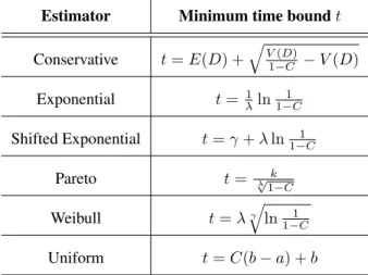
The same logic was applied to define bound estimators for the other four dis-tributions. The six estimators are presented in Table 2.
4.4 Selection Logic
As explained in Section 4.1, the phase detection mechanisms are individually exe-cuted and each one indicates the environment condition (transient or stable period) and returns one distribution which best characterizes the analyzed history trace whenever a stable phase is detected. The selection logic receives the mechanisms results and is responsible for selecting one of them as the output of the QoS adap-tation framework (see Figure 2). Since our objective is to produce improved secure bounds, the lowest bound is selected and returned to the client application.
Table 2: Bound estimators for a required coverage C
Estimator Minimum time bound t
Conservative t = E(D) + q V (D) 1−C − V (D) Exponential t = 1 λln1−C1 Shifted Exponential t = γ + λ ln1−C1 Pareto t = k λ √ 1−C Weibull t = λγ q ln 1 1−C Uniform t = C(b − a) + b
5 Results and Evaluation
The main objective of our work is to show the possibility of having a component which is able to characterize the current state of the environment and, based on dependability objectives of the application, infer how dependability-related bounds should be adapted.
We have introduced the QoS adaptation framework in the previous sections, describing its objectives, functionalities, implemented methods, and algorithms. This section presents a set of results obtained with this framework, and a systematic evaluation focusing on the following main points:
• Validation of our implementation and demonstration of its correctness by
comparing the ability of both mechanisms to characterize the current condi-tions of the environment using controlled traces, synthetically produced;
• Quantification of the framework’s achievements by determining the real
ef-fectiveness and improvements obtained, using real RTT (round-trip time) traces;
• Quantification of the overhead and demonstration of the practical
applica-bility of the framework through a complexity analysis of the implemented algorithms and effective latencies using typical computing platforms.
5.1 Analysis of the phase detection mechanisms
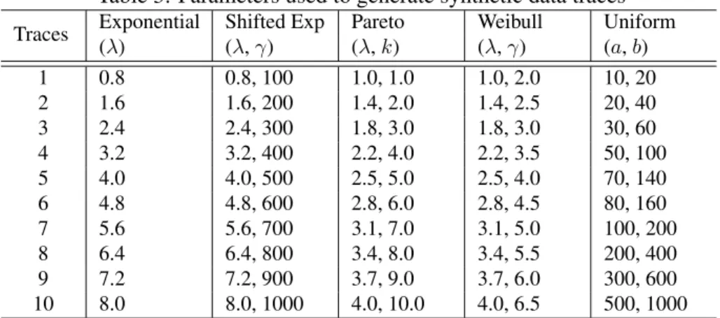
In this first part of our evaluation, we tested the QoS adaptation framework using synthetic data traces in order to analyze the functioning of the AD and KS phase detection mechanisms. We generated 10 traces of 3000 samples for each one of the five considered distributions (exponential, shifted exponential, Weibull, Pareto and uniform). The distributions parameters were configured according to Table 3.
Table 3: Parameters used to generate synthetic data traces
Traces Exponential Shifted Exp Pareto Weibull Uniform
(λ) (λ, γ) (λ, k) (λ, γ) (a, b) 1 0.8 0.8, 100 1.0, 1.0 1.0, 2.0 10, 20 2 1.6 1.6, 200 1.4, 2.0 1.4, 2.5 20, 40 3 2.4 2.4, 300 1.8, 3.0 1.8, 3.0 30, 60 4 3.2 3.2, 400 2.2, 4.0 2.2, 3.5 50, 100 5 4.0 4.0, 500 2.5, 5.0 2.5, 4.0 70, 140 6 4.8 4.8, 600 2.8, 6.0 2.8, 4.5 80, 160 7 5.6 5.6, 700 3.1, 7.0 3.1, 5.0 100, 200 8 6.4 6.4, 800 3.4, 8.0 3.4, 5.5 200, 400 9 7.2 7.2, 900 3.7, 9.0 3.7, 6.0 300, 600 10 8.0 8.0, 1000 4.0, 10.0 4.0, 6.5 500, 1000
The framework was executed for each trace using the phase detection mech-anisms individually. For these executions we defined h = 30 (history size) and
C = 98% (minimum required coverage). Both mechanisms have a parameter
called significance level (α), which defines the probability of not detecting a stable phase. In our experiments we set α = 0.05. We specified four metrics to compare AD and KS goodness-of-fit tests:
• Stability detection: percentage of the sample points that were detected as
stable phases.
• Correct detection: percentage of the sample points characterized as
sta-ble phases in which the framework detected the correct distribution. Given that in this phase of the evaluation we used synthetic traces generated from known distributions, we are able to quantify the correctness of the mecha-nisms.
• Improvement of bounds: improvement obtained with the adaptive approach
in comparison with the conservative one. The improvement is calculated based on the difference between adaptive and pessimistic bounds.
• Coverage: achieved coverage.
Table 4 presents the average results, which show that there is not a single best goodness-of-fit test for all distributions. Actually, the performance of each mech-anism depends on its intrinsic features and on the distribution characteristics. Be-sides, the definition of the best mechanism is related to the evaluation criteria to be verified.
The most important result to be observed in these values is that the two main objectives of the proposed framework were achieved for all distributions by both mechanisms: the bounds were improved (up to 35%) and the minimum required coverage (98%) was secured. In order to fully understand the values presented in
Table 4: Comparing phase detection mechanisms using synthetic data traces
Distribution Stability det. Correct dist. Improvement Coverage
AD KS AD KS AD KS AD KS Exponential 94.53 93.53 98.64 99.19 20.16 19.90 99.58 99.59 Shifted exp. 98.98 99.07 99.18 63.04 1.98 2.12 99.10 98.96 Pareto 76.26 81.75 72.96 78.41 23.62 27.20 98.33 98.25 Weibull 98.43 97.86 79.88 92.63 32.57 35.35 99.41 99.34 Uniform 55.57 48.39 94.82 70.58 9.60 7.50 100.00 100.00
Table 4 and verify the correctness of the mechanisms to characterize the environ-ment, it is necessary to perform a more detailed analysis, separated by distribution. In the experiments with exponential traces, both mechanisms reached excellent and very similar results: they detected stability in more than 90% of the sample points, and correctly characterized almost all of these stable points as exponentially distributed. This significant rate of exponential detection allowed a reduction of approximately 20% in the bounds computed by the framework (comparing to the conservative bounds).
Regarding the shifted exponential distribution, almost all points were detected as belonging to stable phases by the two mechanisms. However, the KS mecha-nism made incorrect characterizations (recognizing other distributions instead of the shifted exponential) in more than 35% of these points. There are at least two factors that can lead to these mistakes: the inherent uncertainty associated with pa-rameters estimation and the probabilistic mechanisms, and the similarities between the tested distributions (e.g. the shifted exponential distribution is an exponential distribution with an extra location parameter, and every exponential distribution is also a Weibull distribution with λ = 1), which is interesting in order to verify the precision of the implemented mechanisms, but also increases the possibility of inaccurate detection. Despite of all these uncertainties, the characterization was correct in the majority of the sample points. Another important observation in the shifted exponential results is that while there was a high rate of stability detection, the improvement of bounds was not significant (2%), showing that the bounds pro-duced by the framework to the shifted exponential distribution are very close to the conservative bounds.
The tests with Pareto traces presented the lowest rate of correct detection among all distributions. This is due to the technical limitation explained in Section 4.1: both mechanisms have Pareto critical values only for a small set of shape param-eters. Thus, besides the uncertainty already present in the parameter estimation, this estimator is rounded to one of these pre-defined values, compromising the ac-curacy of the characterization. However, even with this limitation, the obtained improvement of bounds for the Pareto traces was very significant (about 25% in average).
Both mechanisms presented very good results in the experiments with Weibull traces. Excellent rate of stability detection (more than 95%), good distribution
characterization (80% - 90%) and the best rate of improvement of bounds (up to 35%). These are the best overall results among the tested distributions.
Finally, the results of the tests using uniform traces show that the stability de-tection for this distribution is the more conservative: around 50%. The AD test correctly characterized these sample points as uniformly distributed. We did not obtained the same results with the KS test, which is a good example of the KS limitation: estimating parameters from the sample is not adequated when applying the standard test. As described in Section 4.1, we did not find a modified table of KS critical values for testing uniformity, so we decided to use the general KS table. Consequently, this test failed in detecting the uniform distribution in approximately 30% of the stable points. Nevertheless, both mechanisms obtained almost 10% of improvement in the produced bounds.
From these results, we conclude that it is possible to define effective
mech-anisms to detect stable and transient phases and, for the stable ones, correctly characterize the observed probabilistic distribution.
5.2 Validation using real RTT measurements
This section presents a set of experiments based on real data, in order to prove that our assumption about the interleaved stochastic behavior is realistic for network delays in different environments and demonstrate that our framework is able to characterize these behaviors and provide applications with improved and depend-able time bounds. We selected data traces freely availdepend-able in the Internet, composed by measurements collected in different wired and wireless networks, and extracted RTT traces from them using the tcptrace tool. These RTT traces have been pro-vided as input to our framework (they constitute the “input samples” of Figure 2). Data traces were gathered from the following sources:
• Inmotion: Traceset of TCP transfers between a car traveling at speeds from
5 mph to 75 mph, and an 802.11b access point. The experiments were per-formed on a traffic free road in the California desert. For our tests, we se-lected traces from experiments simulating FTP file transfers. A complete description of the environment, hardware and software used to generate this traceset can be found in [13]. We downloaded the tcpdump files from [12].
• Umass: A collection of wireless traces from the University of Puerto Rico.
Contains wireless signal strength measurements for Dell and Thinkpad lap-tops. Tests were performed over distances of 500 feet and one mile. For more information, see [33].
• Dartmouth: Dataset including tcpdump data for 5 years or more, for over
450 access points and several thousand users at Dartmouth College. We downloaded for our tests a traceset composed by packet headers from wire-less packets sniffed in 18 buildings on Dartmouth campus [18]. Experiments details are discussed in [14].
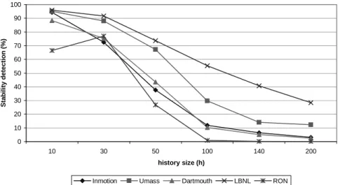
0 10 20 30 40 50 60 70 80 90 100 10 30 50 100 140 200 history size (h) S ta b il it y d e te c ti o n ( % )
Inmotion Umass Dartmouth LBNL RON
Figure 3: Stability detection using different history sizes
• LBNL: Packet traces from two internal network locations at the Lawrence
Berkeley National Laboratory (LBNL) in the USA, giving an overview of internal enterprise traffic recorded at a medium-sized site. The packet traces span more than 100 hours, over which activity from a total of several thou-sand internal hosts appears. These traces are available to download in [23].
• RON: Traces containing thousands of latency and loss samples taken on the
RON testbed. A RON (Resilient Overlay Network) is an application-layer overlay on top of the existing Internet routing substrate, which has the the ability to take advantage of network paths to improve the loss rate, latency, or throughput perceived by data transfers. More information can be found in [1]. The dataset is available in [28].
For the tests with real traces, the phase detection mechanisms were executed in parallel, as illustrated in Figure 2. The most important parameter that must be defined by the framework’s clients is the history size. This parameter states the number of recently collected sample points that are analyzed in the environment characterization, exhibiting a high impact on the results. For this reason, we con-duced a set of experiments with different history sizes for all traces. For these experiments we set the required coverage to C = 0.98, and selected four traces from each data source, with different sizes (10000 to 50000 sample points). The average results for each data source are presented in Figures 3, 4, and 5.
The effects of increasing the history size are perceptible on the obtained val-ues: Figure 3 shows that the higher the history size is, the lower is the rate of stable phases detection. The capacity of correctly identifying stable phases is dependent on the correlation between the sample points, i.e., they need to be collected in a sufficiently recent and small interval of time. Assuming that this correlation is good enough to our purposes (see “sufficient activity” assumption), the inability of
0 5 10 15 20 25 30 10 30 50 100 140 200 history size (h) Im p ro v e m e n t o f b o u n d s ( % )
Inmotion Umass Dartmouth LBNL RON
Figure 4: Improvement of bounds using different history sizes
94 95 96 97 98 99 100 10 30 50 100 140 200 history size (h) A c h ie v e d c o v e ra g e ( % )
Inmotion Umass Dartmouth LBNL RON
Figure 5: Achieved coverage using different history sizes
detecting stable phases when using higher history sizes is explained by the diffi-culty of fitting a large set of samples into one specific distribution. In other words, more sample points increases the possibility that this sample covers environment changes, representing two or more different conditions. Furthermore, detecting less stable phases compromises the average improvement of bounds (Figure 4), because in transient periods there is no improvement at all - the framework com-putes the conservative bound.
On the other hand, if a too small history sample is analyzed, possibly the lack of information leads to serious errors: the mechanisms incorrectly identify stable periods that do not correspond to the real environment conditions. This kind of error compromises the dependability of our approach, because the framework will
input : coverage, history size, measured samples output: New computed bound
1 foreach phase detection mechanism M do 2 Get distribution from M
3 end
4 Select one distribution according to the selection logic 5 Compute new bound based on the required coverage 6 Return new bound
Figure 6: Framework’s algorithm
produce lowest bounds to the identified distribution, generating timing faults and decreasing the overall coverage. This effect can be observed in our experiments with h = 10: in the majority of the traces, they have the highest rate of stability detection (Figure 3) and consequently the best improvement of bounds (Figure 4), but the coverage is not secured (Figure 5).
For all performed experiments, the best results were obtained with history size
h = 30: highest improvement of bounds, securing the minimum required coverage.
These results suggest that there are real environments in which our assumptions
hold. In these environments, the QoS adaptation framework can be successfully
applied in order to make estimations through a probabilistic analysis of historical data and provide applications with better information related to the environment behavior (e.g., network delays), while ensuring the same level of dependability.
5.3 Complexity analysis
One essential factor to be considered in our work is the complexity of the imple-mented algorithms. Although we are assuming that there are enough resources to perform the necessary computations (see Section 3.1), it is important to demon-strate that the framework has an acceptable complexity in order to reach its objec-tives. This section presents an informal analysis of the QoS adaptation framework complexity and some measures of its execution time.
We show that our current framework implementation presents a complexity
O(m×d×h log(h)), where m is the number of phase detection mechanisms based
on GoF tests, d is the number of considered distributions, and h is the history size. The general framework algorithm is described in Figure 6. Assuming that line 2 is a single operation, the complexity of the entire algorithm would be O(m).
However, the execution of a phase detection mechanism (line 2) is not com-posed by one single operation, as shown in Figure 7. This simple algorithm has one for loop, and two conditional tests. The conditional test in line 3 includes the GoF test, which is performed for each distribution to verify if a given sample fits in some assumed distribution (complexity O(d)).
input : measured samples output: detected distribution
1 detected distribution = none 2 foreach distribution D do 3 if samples fit in D then
4 Update detected distribution according to the mechanism’s logic
5 end
6 end
7 if detected distribution = none then 8 return transient phase
9 else
10 return detected distribution 11 end
Figure 7: Phase detection mechanism’s algorithm input : assumed distribution, measured samples
output: if the measures samples fit in the assumed distribution 1 Sort measured samples
2 Calculate GoF statistic S for assumed distribution ˆD
3 Get critical value ch,α 4 if S ≤ ch,αthen 5 return true 6 else
7 return false 8 end
Figure 8: GoF test’s algorithm
A general algorithm of GoF tests is presented in Figure 8 (the specific algo-rithms of the two GoF tests implemented in our framework were described in Sec-tion 4.1). For both mechanisms, in order to calculate the GoF statistic (line 2), it is necessary to sort the input sample and estimate the distributions parameters. Our implementation uses a modified mergesort with complexity O(h log(h)) to sort the measured data (line 1), where h is the history size.
Regarding parameters estimation, the exponential distribution has only one pa-rameter (λ), which is estimated as the inverse of the sample mean. This estimation has a complexity that is linear with the history size (O(h)). The shifted exponen-tial parameters (λ and γ) and the Weibull parameters (α and γ) are estimated using linear regression, which also has linear complexity with the history size O(h). The
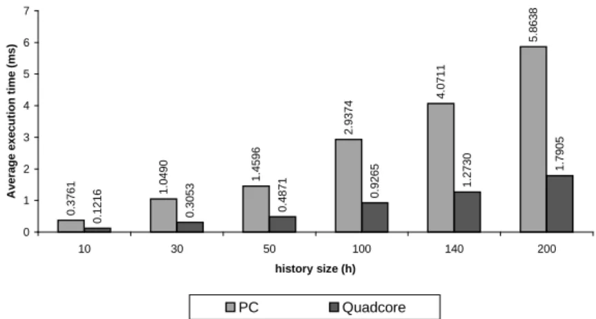
0 .3 7 6 1 1 .0 4 9 0 1 .4 5 9 6 2 .9 3 7 4 4 .0 7 1 1 5 .8 6 3 8 0 .1 2 1 6 0 .3 0 5 3 0 .4 8 7 1 0 .9 2 6 5 1 .2 7 3 0 1 .7 9 0 5 0 1 2 3 4 5 6 7 10 30 50 100 140 200 history size (h) A v e ra g e e x e c u ti o n t im e ( m s ) PC Quadcore
Figure 9: Achieved coverage using different history sizes
k parameter of the Pareto distribution is estimated as the smallest sample value
and the α parameter is computed using a MLE formula. Both estimations are performed with complexity O(h). Finally, the uniform parameters a and b are esti-mated as the minimum and maximum sample values, leading to a O(h) complexity. Moreover, the formulas presented in Section 4.1 to compute the GoF statistics are also calculated in linear time (O(h)). Thus, performing a Gof test takes h log(h)+h operations, which is reduced to an asymptotic complexity of O(h log(h)).
Since the GoF test’s algorithm is executed for each distribution D and for each detection mechanism M , we conclude that the complexity of the current imple-mentation of the QoS adaptation framework is O(m × d × h log(h)), as previ-ously mentioned. Considering a fixed number of mechanisms and distributions (in the current implementation, m = 2 and d = 5), the actual complexity of the framework execution is O(h log(h)). It is important to note that this complexity is imposed by the sort operation required by both mechanisms.
We also measured the time that the framework takes to compute a new bound, for different history sizes. The measurements were performed in two different plat-forms: (i) a Dell Optiplex GX520 PC, with 2GB of RAM and one 2.8GHz Pentium 4 processor, and (ii) a 64-bit 2.3GHz quadcore Xeon machine. The initial point (time 0) is the one where the framework has the sample trace available in a list, and the final point is defined immediately after a new bound is produced. To execute these tests we variated the history size from 10 to 200 and used an Inmotion trace composed by 8200 points, generating approximately 8000 new bounds. Figure 9 presents the average execution times for each history size, using both platforms.
The analysis of the execution time can be helpful in order to determine how a certain application should use our framework. Ideally, a new bound would be computed whenever a new measured sample is added to the history. However, if new data is added to the history too frequently (a new bound is measured before the framework finishes the previous calculation), then the service requests should be adapted to this scenario. For example, a new bound could be produced in fixed
intervals, or when n new values were added to the history.
6 Conclusions
In this paper we addressed the problem of supporting adaptive systems and appli-cations in stochastic environments, from a dependability perspective: maintaining correctness of system properties after adaptation. We started from the observation that the scene in open distributed applications such as those running in IP-based and/or complex embedded systems, is under important factors of change: (i) those under traditionally weak models, such as asynchronous, are under increasing per-formance demands, which lead to sometimes hidden timing/synchrony assump-tions; (ii) those under traditionally strong models, such as hard real-time or syn-chronous, are under increasing demands for dynamic behaviour or configuration.
This is leading to increased threats to system correctness, such as failures due to impossibility results in asynchronous systems, or failures due to missed dead-lines and bounds in synchronous ones, respectively. Clearly, the key issue in these problems is the lack, or loss thereof, of coverage of time-related assumptions.
We proposed to overcome these problems by securing coverage stability. With this, we aim at ensuring automatic adaptation of time-sensitive applications whilst safeguarding correctness, despite variations of aprioristic assumptions about time. Therefore, while other works addressing adaptive systems are mainly concerned with performance, our main concern is dependability.
We advanced on previous work by leveraging on the assumption that i) a system alternates stable periods, during which the environment characteristics are fixed, and unstable periods, in which a variation of the environment conditions occurs, and ii) that the mode changes can be detected. Based on that, we proposed and evaluated a general framework for adaptation, which allows to dynamically set op-timistic time bounds when a stable phase is detected, while it provides conservative but still dependable bounds during transient phases.
We believe that the fundamental conclusion to derive from the full set of exper-iments reported in this paper, is that it is possible to define effective mechanisms to detect stable and transient phases and, for the stable ones, correctly characterize the observed probabilistic distribution. Because of that, the proposed framework constitutes a promising approach to achieve dependable adaptation and, at the same time, obtain improved (tighter) time bounds than those previously obtained with a more conservative approach. This improvement is relevant in the implementation of practical systems, for instance in the configuration of timeouts in failure detec-tors, where the objective is to use the smallest possible time bound (to improve the detection time) without compromising the failure detector accuracy (mistakes due to timing faults).
Furthermore, the experiments performed using real data collected in different environments demonstrate that: a) the assumptions stated in this paper are met in real systems; and b) the framework is actually configurable for specific
envi-ronments. We also presented an informal complexity analysis which is sufficient to show that our solution presents a good performance and satisfactory execution times.
Acknowledgments
This work was partially supported by the EC, through project IST-FP6-STREP-26979 (HIDENETS), and by the FCT, through the Multiannual and CMU-Portugal programmes.
References
[1] David Andersen, Hari Balakrishnan, Frans Kaashoek, and Robert Morris. Re-silient overlay networks. SIGOPS Oper. Syst. Rev., 35(5):131–145, 2001. [2] N. Balakrishnan and A.P. Basu. The exponential distribution: Theory,
meth-ods and applications. CRC Press, 1995.
[3] Jean-Chrysostome Bolot. Characterizing end-to-end packet delay and loss in the internet. Journal of High Speed Networks, 2:305–323, 1993.
[4] G. C. Buttazzo. Hard real-time computing systems. Kluwer Academic Pub-lishers, 1997.
[5] A. Casimiro, P. Lollini, M. Dixit, A. Bondavalli, and P. Verissimo. A frame-work for dependable qos adaptation in probabilistic environments. In 23rd
ACM Symposium on Applied Computing, Dependable and Adaptive Dis-tributed Systems Track, pages 2192–2196, Fortaleza, Ceara, Brazil, March
2008.
[6] A. Casimiro and P. Verissimo. Using the Timely Computing Base for De-pendable QoS Adaptation. In Proceedings of the 20th IEEE Symposium on
Reliable Distributed Systems, pages 208–217, New Orleans, USA, October
2001.
[7] W. Chen, S. Toueg, and M. K. Aguilera. On the quality of service of failure detectors. IEEE Trans. Comput., 51(1):13–32, 2002.
[8] A. Corlett, D.I. Pullin, and S. Sargood. Statistics of one-way internet packet delays, March 2002. http://www.potaroo.net/ietf/all-ids/draft-corlett-statistics-of-packet-delays-00.txt.
[9] Allen B. Downey. Evidence for long-tailed distributions in the internet. In
IMW ’01: Proceedings of the 1st ACM SIGCOMM Workshop on Internet Measurement, pages 229–241, New York, NY, USA, 2001. ACM.
[10] T. Elteto and S. Molnar. On the distribution of round-trip delays in tcp/ip net-works. In Local Computer Networks, 1999. LCN ’99. Conference on, pages 172–181, 1999.
[11] James W. Evans, Richard A. Johnson, and David W. Green. Two- and three-parameter weibull goodness-of-fit tests. FPL-RP-493, 1989; Forest Products Laboratory Research Paper, 1989.
[12] Richard Gass, James Scott, and Christophe Diot. CRAWDAD
trace set cambridge/inmotion/tcp (v. 2005-10-01). Downloaded from http://crawdad.cs.dartmouth.edu/cambridge/inmotion/tcp, October 2005. [13] Richard Gass, James Scott, and Christophe Diot. Measurements of in-motion
802.11 networking. In WMCSA ’06: Proceedings of the Seventh IEEE
Work-shop on Mobile Computing Systems & Applications, pages 69–74,
Washing-ton, DC, USA, 2006.
[14] Tristan Henderson, David Kotz, and Ilya Abyzov. The changing usage of a mature campus-wide wireless network. In MobiCom ’04: Proceedings of the
10th annual international conference on Mobile computing and networking,
pages 187–201, 2004.
[15] J. A. Hernández and I. W. Phillips. Weibull mixture model to characterise end-to-end internet delay at coarse time-scales. IEE Proc. Communications, 153(2):295–304, April 2006.
[16] R. Jain. The Art of Computer Systems Performance Analysis. John Wiley and Sons, 1991.
[17] H. Kopetz and G. Bauer. The Time-Triggered Architecture. Proceedings of
the IEEE, 91(1):112–126, Jan 2003.
[18] David Kotz, Tristan Henderson, and Ilya Abyzov. CRAWDAD
trace set dartmouth/campus/tcpdump (v. 2004-11-09). Downloaded
from http://crawdad.cs.dartmouth.edu/dartmouth/campus/tcpdump, Novem-ber 2004.
[19] J.W.S. Liu. Real-time systems. Prentice Hall, 2000.
[20] Athina Markopoulou, Fouad A. Tobagi, and Mansour J. Karam. Loss and delay measurements of internet backbones. Computer Communications,
29(10):1590–1604, June 2006.
[21] M. Menth, J. Milbrandt, and J. Junker. Time-exponentially weighted moving histograms (TEWMH) for application in adaptive systems. In Proceedings of
the Global Telecommunications Conference (GLOBECOM ’06), pages 1–6,
[22] K. Papagiannaki, S. Moon, C. Fraleigh, P. Thiran, and C. Diot. Measurement and analysis of single-hop delay on an ip backbone network. IEEE Journal
on Selected Areas in Communications. Special Issue on Internet and WWW Measurement, Mapping, and Modeling, 21(6):908–921, August 2003.
[23] Vern Paxson, Ruoming Pang, Mark Allman, Mike Bennett, Jason Lee, and Brian Tierney. lbl-internal.20041004-1303.port001.dump.anon (package). http://imdc.datcat.org/package/1-507R-8=lbl-internal.20041004-1303.port001.dump.anon, 2007.
[24] N.M. Piratla, A.P. Jayasumana, and H. Smith. Overcoming the effects of cor-relation in packet delay measurements using inter-packet gaps. In
Proceed-ings of the 12th IEEE International Conference on Networks (ICON 2004),
pages 233–238, November 2004.
[25] III Porter, J.E., J.W. Coleman, and A.H. Moore. Modified ks, ad, and c-vm tests for the pareto distribution with unknown location and scale parameters.
Reliability, IEEE Transactions on, 41(1):112–117, Mar 1992.
[26] Mezbahur Rahman, Larry M. Pearson, and Herbert C. Heien. A modified anderson-darling test for uniformity. Bulletin of the Malaysian Mathematical
Sciences Society, 29(1):11–16, 2006.
[27] ReliaSoft. Using rank regression on y to calculate the
pa-rameters of the weibull distribution - reliasoft corporation.
http://www.weibull.com/LifeDataWeb/
estimation_of_the_weibull_parameter.htm, 2006.
[28] MIT RON. Ron - resilient overlay networks. http://nms.csail.mit.edu/ron, 2001.
[29] M. A. Stephens. Edf statistics for goodness of fit and some comparisons.
Journal of the American Statistical Association, 69(347):730–737, sep 1974.
[30] M. A. Stephens. Asymptotic results for goodness-of-fit statistics with un-known parameters. Annals of Statistics, 4:357–369, 1976.
[31] O. Tickoo and B. Sikdar. Queueing analysis and delay mitigation in ieee 802.11 random access mac based wireless networks. In INFOCOM 2004.
Twenty-third AnnualJoint Conference of the IEEE Computer and Communi-cations Societies, volume 2, pages 1404–1413 vol.2, March 2004.
[32] K. S. Trivedi. Probability and Statistics with Reliability, Queuing and
Com-puter Science Applications. John Wiley and Sons, 2002.
[33] UMass Trace Repository. UPRM wireless traces. Downloaded from
[34] P. Verissimo and A. Casimiro. The Timely Computing Base model and archi-tecture. Transactions on Computers - Special Issue on Asynchronous
Real-Time Systems, 51(8):916–930, August 2002.
[35] M. Yang, X. R. Li, H. Chen, and N. S. V. Rao. Predicting internet end-to-end delay: an overview. In Proc. of the 36th IEEE Southeastern Symposium on