UNIVERSIDADE DE LISBOA
FACULDADE DE CIÊNCIAS
DEPARTAMENTO DE BIOLOGIA VEGETAL
Ocean Colour off the Portuguese Coast: Chlorophyll a products
validation and applicability
Carolina Garcia Vieira de Sá
DOUTORAMENTO EM CIÊNCIAS DO MAR
UNIVERSIDADE DE LISBOA
FACULDADE DE CIÊNCIAS
DEPARTAMENTO DE BIOLOGIA VEGETAL
Ocean Colour off the Portuguese coast: Chlorophyll a products
validation and applicability
Carolina Garcia Vieira de Sá
Tese orientada pela Prof. Doutora Vanda Brotas e pelo Prof. Doutor José da Silva, especialmente elaborada para a obtenção do grau de doutor em
Ciências do Mar.
Declaration
According to Chapter V, article 40, paragraph 1 of the Regulation concerning Post-Graduate Studies at the University of Lisbon, which was published in the Portuguese Republic’s Official Journal (Series II, no153, of 5 July 2003), the PhD candidate hereby declares that she participated in the designing and carrying out the field work, as well as in interpreting the results, and drafting the manuscripts to be submitted for publication.
Carolina Sá Lisboa, 19 October 2013
This study was performed in the framework of HabSpot FCT Project, PTDC/MAR/100348/2008 and European Space Agency projects DUE CoastColour (ESRIN/AO/1-6141/09/l-EC) and Climate Change Iniciative – Ocean Colour (AO-1/6207/09/I-LG). The work has been also partially supported by the European Space Agency within the framework of the MERIS Validation Activities under contract n. 12595/09/I-OL, and sampling activities benefited from European projects HERMES (GOCE-CT-2005-511234) and Hermione (EC contract 226354) support. The candidate received a PhD grant from the Portuguese Science Foundation (FCT-SFRH/BD/24245/2005).
Parts of the work and dataset presented in this thesis have been considered and included in the following international publications:
1. Sá, C., da Silva, J.C.B., Oliveira, P.B., Brotas, V. (2008). Comparison of MERIS (ALGAL_1 and ALGAL_2) and MODIS (OCM3) of chlorophyll products and validation with HPLC in situ data collected off the Western Iberian Peninsula. Proceeding of the 2nd
MERIS/(A)ATSR Workshop. ESA, SP-666.
2. Ruddick, K., Brockmann, C., Doerffer, R., Lee, Z., Brotas, V., Fomferra, N., Groom, S., Krasemann, H., Martinez-Vicente, V., Sá, C., Santer, R., Sathyendranath, S., Stelzer, K., Pinnock, S. (2010). The Coastcolour project regional algorithm round robin exercise.
Remote Sensing of the Coastal Ocean, Land, and Atmosphere Environment. Incheon, South Korea, October 13-14, 2010. Proceedings of SPIE, the International Society for Optical Engineering, 7858: pp. DOI: 10.1117/12.869506.
3. Mendes, C.R., Sá, C., Vitorino, J., Borges, C., Garcia, V.M.T., Brotas, V.(2011) Spatial distribution of phytoplankton communities in the Nazaré submarine canyon region (Portugal): HPLC-CHEMTAX approach. Journal of Marine Systems 89 (1):90-101.
4. Brotas, V., Brewin, R., Sá, C., Brito, S., Silva, A., Mendes, R., Diniz, T., Kaufmann, M., Tarran, G., Groom, S., Platt, T., Sathyendranath, S. (2013). Approaches to derive phytoplankton functional types and size classes. Validation along a gradient of trophic status in Eastern Atlantic. Remote Sensing of Environment, 134, 66-77.
5. Brito, A., Sá, C., Brotas, V., Vitorino, J., Platt, T., Sathyendranath, S. (under revision). Understanding bio-optical properties of phytoplankton in the western Iberian coast: application of theoretical models. Remote Sensing of Environment.
6. Sá, C., D’Alimonte, Brito, A., Kajiyama, T., Zibordi, G., Mendes, C.R., Bherton, J-F., Canutti, E., Oliveira, P., da Silva, J., Brotas, V. (in preparation). Validation of satellite ocean colour chlorophyll products for the Western Iberia: comparison of algorithms. 7. Sá, C., D’Alimonte, Brito, A., Kajiyama, T., Zibordi, G., Bherton, J-F., Canutti, E., da Silva,
J., Brotas, V. (in preparation). Temporal and spatial variability of case I waters off the Western Iberia.
Acknowledgements
The decision to embrace a doctoral programme implies a commitment that is not possible just with the individual effort but needs the comprehension and support by colleagues and family. It is a long journey full of expectations, uncertainties and surprises. It is also a learning process in maturing to become a true scientist. In the next lines I would like to express my gratitude to all that to some extent contributed to the elaboration of this thesis.
I am thankful to my advisors, Prof. Vanda Brotas and Prof. José da Silva for their trust, scientific advisory and unconditional support. Thank you for giving me the opportunity to participate in multidisciplinary projects and never doubting my capabilities.
I am deeply grateful to Davide D’Alimonte whose expertise, and scientific discussions added considerably to my experience. Thank you so much for your kindness and for being an inspiration.
I express my most sincere gratitude to Ana Brito for her friendship and support throughout the writing process of this thesis. Thank you also for always challenging me into new projects.
To Ana Sousa and Rafael Mendes, who have been with me since the beginning of this scientific journey, I send a warm thank you for their friendship and encouragement. I also thank Tamito and his beautiful family for their support and happy times together.
I would like also to send a word of appreciation to all of those who have shared with me their laboratory experience and expertise, and to those who have spent with me hours of sampling, hours of joy and hard work while at sea. A thank you note to Alexandra Silva, Bruno Jesus, Carla Gameiro, Catarina Guerreiro, Inês Martins, Lourenço Ribeiro, Miguel Leal, Paulo Cartaxana, Sérgio Muacho, Teresa Silva and Vera Veloso.
A special thanks to Henko De Stigter, João Vitorino and Teresa Moita, for the opportunity to participate in their scientific cruises. Sampling would have not been possible without their support. Furthermore I would also like to acknowledge with much appreciation the crucial role of Jean-Paul Huot and Giuseppe Zibordi who made the optical sampling campaign possible.
Finally, a huge thanks to my dearest friends: Rita, Filomena, Ana Rita and Maria João, and to my big and lovely family, without whom this thesis would have not been possible. Life is so much funnier when you are around. Thank you for your daily support and encouragement.
Index
Resumo ... 23
Summary... 27
Thesis motivation, objectives and outline ... 29
Chapter 1: Introduction ... 31
1.1 Ocean colour ... 33
1.1.1 Electromagnetic radiation and optical properties ... 33
1.1.2 Water types ... 38
1.1.3 Ocean colour algorithms ... 42
1.1.4 Ocean colour sensors ... 43
1.1.5 Ocean colour products validation ... 45
1.2 Phytoplankton ... 45
1.2.1 Phytoplankton: size classes and functional types ... 46
1.2.2 Phytoplankton Pigments ... 47
1.2.3 Phytoplankton from space ... 50
1.3 Study site ... 51
Chapter 2: Data and Methods ... 57
2.1 In situ data: sampling and processing ... 59
2.1.1 Phytoplankton pigments ... 59
2.1.2 Phytoplankton absorption spectra ... 64
2.1.3 Radiometric data ... 64
2.2 Satellite data ... 65
2.2.1 Standard algorithms ... 65
2.2.2 Novel algorithms ... 68
2.3 Data quality assurance for matchup analysis ... 70
2.3.1 In situ database ... 70
2.3.2 Satellite data ... 70
2.4 Match-up and comparison procedures ... 72
2.5 Statistics formulae ... 73
2.6 Water type index ... 74
Chapter 3: Results ... 79
3.1 Dataset for the western Portuguese waters ... 81
3.2 Match-up analysis of Chlorophyll products ... 86
3.2 1 Standard Chlorophyll products ... 87
3.2.2 Novel Chlorophyll Products ... 91
3.2.2 Comparisons between MERIS and MODIS Standard products ... 98
3.3 Water typology: Case1 vs non-Case1 waters ... 100
3.3.1 Optical properties off the Portuguese coast using in situ data ... 100
3.3.2 Water typology using remote sensing data ... 101
3.3.3 Model constraints and applicability ... 109
3.3.4 Temporal and Spatial variability of Case 1 waters ... 114
3.4 Factors affecting satellite percentage error ... 117
Chapter 4: Discussion ... 121
4.1 In situ dataset ... 123
4.1.1 Chlorophyll a measurement uncertainties ... 123
4.1.2 Geographical and temporal coverage ... 125
4.1.3 Contribution to current knowledge ... 127
4.2 Match-ups ... 130
4.2.1 Analysis constraints ... 130
4.2.2 Assessment of algorithms effectiveness ... 132
4.2.3 Regional analysis ... 138
4.3 Assessment of water typology: Case 1 vs non-Case 1 ... 142
4.3.1 Implications of water typology ... 143
4.3.2 Understanding regional optical properties ... 144
4.3.3 Water typology remote sensing model constraints: atmospheric correction .... 148
4.3.4 Water type temporal and spatial distribution ... 150
4.4 Factors affecting chlorophyll product accuracy ... 153
4.4.1 Index water type ... 153
4.4.2 Phytoplankton size classes ... 154
4.4.3 Other parameters ... 155
Chapter 5: Final remarks ... 159
5.1 General considerations ... 161
Chapter 6: References ... 165 Annex I: Dataset ... 185 Annex II: Case water-type maps ... 217
29
Thesis motivation, objectives and outline
This thesis was motivated by the need to better understand the performance of standard Chlorophyll a (Chl) satellite products. Phytoplankton represent the basis of oceanic food webs. Their dynamics may have significant implications in terms of fisheries and they can be considered as indicators of ecosystem quality. Therefore, they are key elements to evaluate and monitor, both in short and long-term perspectives. The aim of this thesis was to evaluate the standard MERIS and MODIS Chl products, to perform algorithm regional adjustments, and to identify the spatial and temporal variability of environmental parmeters that influence their performance. The main objective was pursued by focusing on the following specific tasks:
①. To gather a phytoplankton pigment database for ocean colour product validation and application development;
②. To validate and compare MERIS and MODIS sensor Chl products for the Portuguese coast;
③. To perform regional adaptations to the algorithms;
④. To provide a classification of the waters off the Portuguese coast and a general seasonal and spatial analysis of its variability.
A schematic representation of the thesis organization is presented in Figure 1. The thesis is organized in 5 Chapters. Chapter 1 includes a general introduction to provide the reader the background and necessary context to understand the work described in the following chapters. Basis of ocean-colour and phytoplankton knowledge are provided, as well as a characterization of the study area. The data collected and methods applied are detailed in Chapter 2. Data collection and quality processing of both in situ and satellite datasets are described. Details on the comparison procedure and statistical analysis are also given. The complete in situ dataset is provided in Annex I. Results are presented in Chapter 3 and discussed in Chapter 4. Concluding remarks, as well as future perspectives are addressed in Chapter 5.
30
Tables Index
Table I List of ocean colour sensors (IOCCG, 2012). ... 44 Table II List of most relevant pigments and their correspondent occurrence in
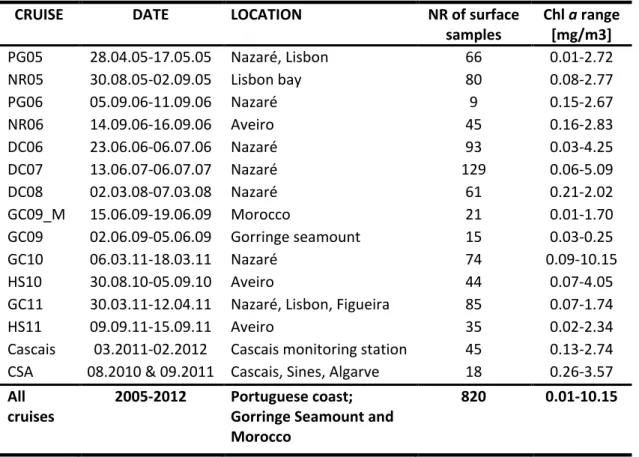
phytoplankton communities (Jeffrey et al., 1997). ... 48 Table III List of oceanographic cruises with respective sampling period, location, number of
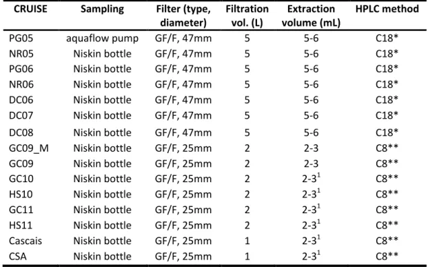
surface samples collected and Chlorophyll a (Chl) values range. ... 60 Table IV Summary of sampling and processing methods used in each cruise. ... 61 Table V List of flags used for processing the satellite data. ... 71 Table VI Summary statistics for linear regression analyses between TChl a and accessory
pigments. ... 81 Table VII Statistical results obtained from the agreement between in situ field data and
concomitant satellite data. ... 88 Table VIII Summary of the diffences (diff) observed between the maps of SeaWiFS and MODIS classification for 2005. Results are presented for each season. ... 106 Table IX Statistics of MODIS radiometric data comparison with the in situ SeaBASS database ... 110 Table X Statistics of SeaWiFS radiometric data comparison with the in situ SeaBASS database ... 111 Table XI Statistics of MODIS radiometric data comparison with in situ data collected off the
Portuguese coast (cruise GC11). ... 112 Table XII Correlation matrices for MODIS and MERIS standard products match-ups parameters. . 119
Figures Index
Figure 1 Schematics of thesis organization and investigated topics. ... 30
Figure 2 Schematic representation of the atmospheric windows for remote sensing. ... 34
Figure 3 Schematics of light pathways reaching a remote sensor. ... 35
Figure 4 Factors that influence the upwelling light leaving the sea surface. ... 39
Figure 5 Reflectance spectra of water masses dominated by different optical active components. ... 40
Figure 6 Water type classification scheme. ... 41
Figure 7 Chlorophyll a structure ... 47
Figure 8 Example of absorption spectra for a range of monospecific cultures. ... 50
Figure 9 The Western Iberia and Gulf of Cadiz regimes in a) spring and summer, and b) autumn and winter. ... 53
Figure 10 Schematics of a deep chlorophyll maximum (DCM). ... 54
Figure 11 Samples location taken on board RV Pelagia in 2005 (PG05) and 2006 (PG06); NI Noruega 2005 (NR05) and 2006 (NR06); NRP D.Carlos I in 2006 (DC06), 2007 (DC07) and 2008 (DC08); NRP Gago Coutinho in 2009 (GC09 and GC09M), 2010 (GC10) and 2011 (GC11); RV Mytilus in 2010 and 2011 under HABSpot project (HS10, HS11) and coastal monitoring stations in Cascais and Cascais, Sines and Algarve (CS and CSA, respectively). ... 59
Figure 12 Lee and Hu 2006 model (result of equation 2.16 and 2.18) ... 75
Figure 13 Lee and Hu 2006 model (result of equation 2.17 and 2.19) ... 75
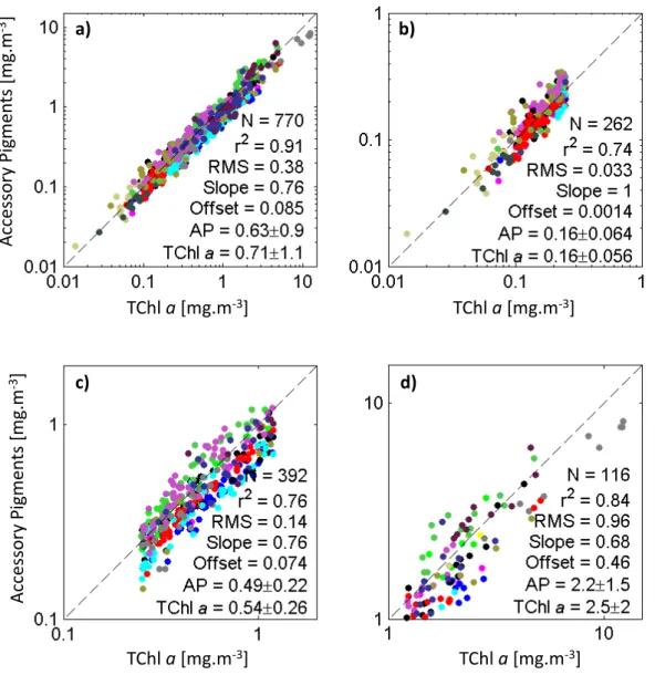
Figure 14 Pigment dataset after quality control: accessory pigments against total chlorophyll a (Tchl a). ... 82
Figure 15 Pigment dataset, after quality control, separated for size class dominance based on Uitz et al., 2006. ... 83
Figure 16 Distribution map of the different size dominant samples (a) and all dataset relation between accessory pigments (AP) and total chlorophyll a (TChl a) (b). . ... 84
Figure 17 Ternary plot showing the relative contributions (percent) of picoplankton, nanoplaknton, and microphytoplankton to total Chl, estimated from the relative contribution of some taxonomic pigments (Uitz et al., 2006). ... 85
Figure 18 Variations of size index (Bricaud et al 2004) as function of chlorophyll (TChla). . ... 86
Figure 19 Match-up results obtained using the standard algorithms for MODIS (OC3M) and MERIS (algal 1 and algal 2). A 3h time difference was used in this analysis. ... 89
Figure 20 Match-up results obtained using the standard algorithms for MODIS (OC3M) and MERIS (algal 1 and algal 2). Two different time intervals are represented: 0 to 3h (black) and 3 to 6h (blue). ... 90
Figure 21 Regional adjustment of the equation 2.8 of the algal 2 Chl product, based on in situ absorption values at 442nm and Chl concentrations (a). Recalculation of match-up results using the regionally adjusted product, in black, and previous results of the standard product, in grey (b). ... 91 Figure 22 Match-up results obtained using the novel products developed in the CoastColour
Project, using MERIS (CC_NN and CC_QAA). A 3h time difference was used in this analysis. . ... 92 Figure 23 Match-up results obtained after regionally adjusting the novel products developed in the CoastColour Project, using MERIS (CC_NN and CC_QAA). A 3h time difference was used in this analysis. . ... 93 Figure 24 Match-up results obtained using the novel algorithms developed for the regionally
adjusted MLP-NN, using MERIS (MLPME_ATLP). A 3h time difference was used in this analysis. ... 94
Figure 25 Match-up results obtained using the novel algorithms developed for the regionally adjusted MLP-NN, using MERIS (MLPME_ATLP). Two different time intervals are represented: 0 to
3h (black) and 3 to 6h (blue). ... 95 Figure 26 Match-up results obtained using the novel algorithm developed for regional adjusted MLP-NN, using MODIS (MLPMO_ATLP). A 3h time difference was used in this analysis. ... 96
Figure 27 Match-up results obtained using the novel algorithms developed the regionally adjusted MLP-NN, using MODIS (MLPMO_ATLP). Two different time intervals are represented: 0
to 3h (black) and 3 to 6h (blue). ... 97 Figure 28 Match-up results obtained with the Chl CCI product. A 3h time difference was used in this analysis. ... 98 Figure 29 Location of common valid pixels using algal 1 and algal 2 MERIS algorithms (a); The
comparison between the Chl product for these two algorithms is also presented (b).. ... 99 Figure 30 Location of common match-ups for MODIS and MERIS (algal 1) products, within a time window of 6h (a). The comparison between the Chl products for these two sensors is also
presented (b). ... 99 Figure 31 Ternary plot of absorption at 442nm of CDOM, non-algal particles and phytoplankton measured during the GC11 cruise. ... 100 Figure 32 All in situ radiometric data collected during the GC11 cruise superimposed with Lee
and Hu (2006) model: a) RR12_RR53 condition, b) Rrs555_RR53 condition. ... 101 Figure 33 Reflectance ratios applied to MODIS (in blue) and SeaWIFS (in black) data off the
Portuguese coast with superimposed Lee and Hu (2006) model for Case 1-waters (lines). Data presented are averaged Rrs data for the Summer period of 2005. ... 102 Figure 34 Maps of percentage of pixel classification as Case 1 waters according to Lee and Hu
(2006) model conditions for MODIS data, considering the four seasons of 2005. ... 103 Figure 35 Maps of percentage of pixel classification as Case 1 waters according to Lee and Hu
(2006) model conditions for SeaWiFS data, considering the four seasons of 2005. ... 104 Figure 36 Maps of the difference between SeaWiFS and MODIS Case 1 waters percentage
d) winter. Note that b) is the result of the difference between Figure 35 b) and Figure 34 b). Positive values result from higher percentage values for SeaWiFS classification and negative
values from higher percentage values of MODIS classification. ... 107 Figure 37 Maps of the difference between SeaWiFS and MODIS Case 1 waters percentage
classification using only the Rrs555_RR53 condition for 2005: a) spring, b) summer, c) autumn and d) winter. ... 108 Figure 38 Validation of radiometric MODIS data with SeaBaSS in situ database. ... 110 Figure 39 Validation of radiometric SeaWiFS data with SeaBaSS in situ database. ... 111 Figure 40 Validation of radiometric MODIS data with in situ data collected during the GC11
cruise. ... 112 Figure 41 RR12 ratio variation with distance from coast (km). ... 113 Figure 42 Radiometric MODIS match-ups with the CO database (n=75), for a 6h time window,
plotted superimposed with the Lee andHu 2006 model (lines). ... 114 Figure 43 Seasonal maps of percentage of pixel classification as Case 1 waters according to Lee and Hu (2006) model conditions for the MODIS data for a 7 years period, 2005-2011. ... 115 Figure 44 Maps of standard deviation of seasonal percentage of pixel classification as Case 1
waters according to Lee and Hu (2006) model (Rrs555_RR53 condition) for the MODIS data for a 7 years period, 2005-2011. ... 116 Figure 45 Mean percentage of total pixels between 2005 and 2011 for each season. ... 117 Figure 46 Target diagram for the relation of each Chl product with their correspondent in situ
match-ups. URMS (∆) is plotted in the x-axis, and bias (δ) in the y-axis. Dotted lines are isolines of RMS (Ψ), as according to equation Ψ2=∆2+δ2. ... 134 Figure 47 Taylor diagram for the relation of each Chl product with their correspondent in situ
match-ups. Normalized standard deviation is plotted in the x-axis, and the angle corresponds to the correlation coefficient. Dashed black lines are isolines of normalized standard deviation, dotted black lines are correlation coefficient isolines and dotted blue lines are isolines of URMS (∆). ... 136 Figure 48 Target diagram for the relation of CoastColour QAA (a) and NN (b) Chl products with their correspondent in situ match-ups. ... 139 Figure 49 Target diagram for the relation of MODIS (a) and CCI (b) Chl products with their
correspondent in situ match-ups. ... 140 Figure 50 Target diagram for the relation of MERIS algal1 (a) and algal2 (b) Chl products with
their correspondent in situ match-ups. ... 141 Figure 51 Target diagram for the relation of MLP_ATLP MO (a) and ME (b) Chl products (novelty index < 3) with their correspondent in situ match-ups. ... 142 Figure 52 Morel and Belanger (2006) model superimposed (for sun-zenith angle of 45°) to
satellite data and Lee and Hu (2006) second condition model. Data presented are averaged Rrs data for the summer period of 2005. ... 151
Figure 53 Variation of percentage error of MODIS matchups with Zeu. ... 157 Figure 54 Summary scheme of comparison between satellite Chl products and the in situ
dataset. Absolute percentage of difference (APD) is presented for each of the standard (in blue) and novel (in green) products tested... 163
23
Resumo
A detecção remota implica que a obtenção de informação sobre um objecto seja feita a distância. Nesse sentido, a informação que se pretende obter tem de estar directamente relacionada com algum parametro mensuravel a essa distância. A medição da “cor” do oceano permite recolher informação sobre as propriedades ópticas de uma determinada massa de agua, uma vez que se encontra directamente relacionada com essas propriedades. Preisendorfer (1961) definiu dois tipos de propriedades opticas para a coluna de agua: as propriedades opticas 1) aparentes e as 2) inerentes. As propriedades aparentes (AOPs), como sejam a reflectância ou a radiância, dependem não só da natureza e quantidade de substâncias presentes, mas são tambem influenciadas pela distribuicao angular do campo de luz. Ao contrario das propriedades inerentes (IOPs), a absorção, dispersão e atenuação, que são independentes das condições de iluminação e dependem somente do tipo e concentração das substâncias presentes na coluna de agua. As substâncias opticamente activas absorvem ou dispersam a luz, podendo as propriedades opticas inerentes serem descritas como a probabilidade de um fotão ser removido (absorvido) ou redireccionado (disperso) por unidade de medida. São estas propriedades que se relacionam directamente com a concentração das substâncias no meio. No entanto, são as propriedades aparentes que são mensuraveis por satelite.
A medição da “cor” é feita pela quantificacao da radiância/reflectância que e emitida pela coluna de agua nos comprimentos de onda do visivel. O sensor óptico, a cerca de 800km de altitude, recebe o sinal emitido. No entanto, 90% do sinal que e recebido provem da atmosfera ou de outras fontes que não da coluna de agua. Diferentes procedimentos foram desenvolvidos para efectuar a correcção atmosferica (ex. Gordon and Wang, 1994) e uma vez isolado o sinal proveniente da coluna de agua, este pode ser então interpretado e relacionado com as suas propriedade ópticas inerentes e consequentemente com as substâncias nela presentes.
Uma única expressão, a radiative transfer equation (RTE), relaciona as propriedades aparentes e inerentes entre si. Contudo, a sua resolução requer o uso de aproximações. Algoritmos empiricos, semi-empiricos e analiticos têm sido desenvolvidos de forma a determinar IOPs e concentrações de substâncias directamente a partir das AOPs medidas pelos sensores (ex.: Garver and Siegel, 1997, Lee et al., 2002, Maritorena et al., 2002, O’Reilly et al., 1998).
Os componentes opticamente activos são geralmente agrupados por semelhanca espectral, e podem ser de 3 tipos: 1) matéria orgânica dissolvida (CDOM), 2) fitoplâncton e 3) material inorgânico particulado (ou sedimentos em suspensão). De forma a simplificar o desenvolvimento
24
de algoritmos, as massas de água foram classificadas em dois tipos (Morel and Prieur, 1977). No caso das aguas tipo-I, as suas propriedades ópticas co-variam com o fitoplancton e material associado. Recorrendo à clorofila (Chl) como proxy, pode afirmar-se que a partir da concentração de Chl se conseguem determinar as propriedades ópticas da massa de água. Quando a presença de CDOM ou de sedimentos em suspensão ocorre simultaneamente e não co-varia com o fitoplâncton, as águas são ditas de tipo-II, e a interpretação das propriedades ópticas é mais complexa.
A clorofila absorve luz predominantemente na região azul e vermelha do espectro do visivel e reflecte na região do verde. Um aumento de Chl conduz a uma diminuição na reflectância na zona do azul e apenas a um ligeiro aumento na região do verde. Estas diferencas de reflectância nos diferentes comprimentos de onda possibilitam o uso dos rácios de reflectância azul-verde para determinar a concentração de Chl através de relações empiricas. Estes algoritmos empiricos são operacionalmente usados pelas Agências Espaciais para gerar produtos de Chl, no entanto, são teoricamente apenas aplicáveis em aguas tipo-I. Em aguas tipo-II, a presença de CDOM ou de sedimentos em supensão pode condicionar a relação dos rácios com a concentração de Chl e portanto, inviabilizar a operacionabilidade destes algoritmos. No entanto, algoritmos aplicaveis em aguas tipo-II têm vindo a ser desenvolvidos (ex.: Doerffer and Schiller, 2007).
As especificidades dos algoritmos podem levar a diferenças nas incertezas dos produtos gerados, e a importância de validar os produtos de Chl com dados in situ de diferentes regiões tem sido reconhecida pelas Agências Espaciais. Estas agências promoveram a criação de bases de dados com o intuito de apoiar a actividade de validação dos seus produtos e de desenvolver novos algoritmos. Os resultados de validação têm revelado que a nivel global os objectivos de exactidão de 5% para os dados radiometricos e de 35% para a concentração de Chl têm sido verificados (McClain, 2009), contudo, a nivel regional, os erros associados podem ser superiores, tendo sido propostos ajustes regionais aos algoritmos (ex.: Garcia et al. 2005, Folkestad et al., 2007, Volpe et al., 2007). O uso dos produtos de Chl para monitorização ambiental, estudos de análise climatológica, ou cálculo de produção primária e análise de impacto dos ciclos bio-geoquimicos a nivel regional e global tornam prioritária a validação e análise de incertezas associadas a estes produtos.
O objectivo principal desta tese incluiu a avaliação dos produtos standard de clorofila dos sensors MERIS e MODIS, o ajuste regional de algoritmos usados para a determinação da concentração de Chl, bem como identificar a variabilidade espacial e temporal dos factores associados aos erros dos produtos de Chl. Os seguintes objectivos especificos foram
25
identificados e realizados: 1) Recolher dados de pigmentos fitoplanctónicos e organizar uma base de dados para a validação e desenvolvimento de aplicações de produtos de “cor” do oceano; 2) Validar e comparar os produtos de Chl dos sensores MERIS e MODIS para a costa portuguesa; 3) Proceder a ajustes regionais dos algoritmos; 4) Produzir mapas de classificação óptica das águas ao largo de Portugal de forma a possibilitar a análise da variabilidade sazonal e espacial da sua distribuição.
A validação dos produtos de Chl para a costa portuguesa foi feita através da análise estatistica da comparação de produtos de diferentes sensores com dados in situ recollhidos durante dois programas de monitorização e a bordo de 13 cruzeiros de investigação. Os dados de pigmentos fitoplanctónicos foram colhidos ao longo dos anos, de 2005 a 2012, e foram processados por cromatografia liquida de alta precisão (HPLC). A concentração de Chl foi comparada com dados contemporaneos dos sensores MERIS e MODIS. Os produtos testados incluiram os produtos
standard algal 1 e algal 2 do MERIS e o OC3M do MODIS, bem como novos produtos,
recentemente desenvolvidos no âmbito de projectos da Agencia Espacial Europeia (ESA), nomeadamente os produtos gerados pelo projecto CoastColour e pelo projecto Climate Change
Iniciative (CCI). O ajuste regional de um algoritmo baseado numa rede neuronal (MLP_ATLP) foi
tambem testado.
De um modo geral, os produtos de satelite revelaram uma sobreestimação da concentração de Chl em comparacao com os valores in situ. Os melhores resultados foram obtidos pelo algoritmo que foi especificamente ajustado para a regiao em estudo (MLP_ATLP). Dos produtos standard testados, os melhores resultados foram determinados com o OC3M do MODIS e o algal 2 do MERIS. O primeiro obteve menor dispersão dos dados (<RMS), o segundo revelou menor erro de exactidão (<bias) em relação aos dados in situ. A análise especifica dos diferentes cruzeiros separadamente revelou diferenças estatisticas, tendo a região da Nazaré sido identificada como uma area de interesse para as actividades de validação. Esta região é oceanograficamente e bio-geoquimicamente muito dinamica, possibilitando a avaliação da performance dos algoritmos em águas com diferentes propriedades ópticas numa reduzida area de amostragem. Dados opticos
in situ foram obtidos durante um cruzeiro nesta região e a análise dos dados revelou a presença
de águas dominadas por CDOM. A informação recolhida neste cruzeiro (68 estacoes de optica), durante a Primavera de 2011, permitiu uma caraterização da região amostrada, no entanto, não possibilita uma generalização, uma vez que a amostragem foi espacial e temporalmente restrita. De forma a obter um mapa da distribuição sazonal dos tipos de água ao longo e ao largo da costa portuguesa, usaram-se dados de detecção remota. O modelo descrito por Lee e Hu (2006)
26
foi testado, mas os resultados revelaram problemas de correcção atmosférica nas primeira bandas do visivel (na região do azul). De qualquer forma, o esquema de classificação dos tipos de agua foi aplicado parcialmente e permitiu mapear a distribuição das águas dominadas por sedimentos em suspensão. A distribuição destas águas revelou uma forte componente sazonal, sendo a sua presença mais predominante ao longo da costa norte, a norte do Cabo Espichel, durante o inverno.
O impacto de diversos parâmetros nos erros determinados para os produtos de Chl foi tambem avaliado. Apenas os produtos standard foram testados e os principais factores associados aos erros determinados variaram de acordo com o produto analisado. Os valores de clorofila, da primeira profundidade óptica e da radiância nos 555 nm foram parâmetros significativamente relacionados com a percentagem de erro encontrada entre o produto MODIS e os dados in situ. Para os produtos standard do MERIS, o erro associado ao produto algal 1 foi significativamente relacionado com o indice de tamanho das celulas da comunidade fitoplanctónica da amostra, com os valores de radiância na banda dos 555 nm e com o rácio das radiâncias nas bandas 412/443nm. Este rácio tambem esteve significativamente relacionado com o erro determinado para o produto algal 2. Os valores de clorofila e da primeira profundidade óptica estiveram tambem significativamente ralacionados com o erro neste produto.
Todos os objectivos inicialmente propostos foram atingidos. Os resultados gerados são essenciais para aplicação em diversas áreas, não só de investigação, mas também como validação de ferramentas de monitorização ambiental. Um exemplo de investigação futura inclui a detecção de blooms de algas nocivas por satélite, o que envolve a análise de dados históricos de Chl, para estabelecer limites associados a variabilidade natural da biomassa fitoplanctónica e identificar anomalias. As contribuições desta tese, serão usadas durante o projecto Europeu EU FP7 AQUA_USERS, cujo objectivo será o de modelar e identificar precocemente o aparecimento deste tipo de blooms, e no qual a equipa do centro de oceanografia está envolvida. A base de dados recolhida durante este estudo pode ainda ser explorada a nivel ecológico e contribuir para o conhecimento da dinâmica das comunidades de fitoplâncton em diferentes regioes da costa portuguesa (ex.: Mendes et al., 2011, Silva et al., 2008).
Palavras-chave: Clorofila, Cor do oceano, deteccão remota, sensores MERIS e MODIS, validacão, características ópticas das massas de água.
27
Summary
Ocean colour is an invaluable tool to monitor temporal and spatial distribution of phytoplankton biomass. Chlorophyll a (Chl) is the main biomass proxy for phytoplankton, and ocean colour sensors allow for a synoptic and quasi-permanent following of this pigment concentration in surface waters. However, algorithms that are designed for use at global scales may be less accurate at local and regional scales, namely in coastal areas. These optically complex areas are of upmost importance to monitor phytoplankton blooms as they are subject to major anthropogenic pressures. Therefore, regional evaluation of products accuracy is needed to ensure correct data analysis and interpretation. It is important to understand the limitations of the different products in reference to specific areas and to validate the ocean-colour standard products with in situ data, in order to satisfy the quality requirements for monitoring purposes. In this thesis, Chl product validation is undertaken by directly comparing remote sensing data with in situ surface data. Water samples collected during 2 monitoring programmes and on board 13 cruises off the Portuguese coast during the period 2005 – 2012 were processed by reversed phase High-Performance Liquid Chromatography (HPLC) for pigment determination, and the Chl concentration compared with coincident MERIS and MODIS sensors data. The performance of standard MERIS (algal1 and algal2) and OC3M MODIS products, as well as novel products generated by ESA projects (i.e., CoastColour and Climate Chnage Initiative, CCI, products) and a regionally adjusted algorithm were evaluated using match-up data sets. In general, satellite products were found to overestimate Chl concentrations in comparison to in
situ values. Best results were determined for the regionalized algorithm (MLP_ATLP) and the
standard products with best results were the MODIS OC3M and the algal 2 MERIS, the former having lower RMS, but the latter revealing lower bias. Statistical differences were verified for the various cruises, and Nazaré region was identified as an area of interest for validation activities due to its complex oceanographic dynamic. Optical in situ data collected in one cruise revealed the presence of CDOM dominated waters, however more comprehensive analysis is needed. The use of remote sensing data for water-type classification revealed the need for improved atmospheric correction in the blue part of the spectrum. Nonetheless, classification scheme applied revealed a strong seasonal component in the spatial distribution of non-case 1 water types, which were more relevant along the northern coast (i.e., north of Cape Espichel) during winter.
28
Factors influencing Chl products accuracy varied according to product under analysis. Biomass, first optical depth and water-leaving radiance at 555 nm were found to be significantly related to the percent error of MODIS Chl product. For MERIS standard products, algal 1 percent error was significantly related to the phytoplankton size index, to the water-leaving radiance at 555 nm and to the water-leaving radiance ratio 412/443 nm, which was also significantly related to the algal 2 product error. Biomass and the first optical depth were the other factors identified to be significantly related to algal 2 product percent error.
29
Thesis motivation, objectives and outline
This thesis was motivated by the need to better understand the performance of standard Chlorophyll a (Chl) satellite products. Phytoplankton represent the basis of oceanic food webs. Their dynamics may have significant implications in terms of fisheries and they can be considered as indicators of ecosystem quality. Therefore, they are key elements to evaluate and monitor, both in short and long-term perspectives. The aim of this thesis was to evaluate the standard MERIS and MODIS Chl products, to perform algorithm regional adjustments, and to identify the spatial and temporal variability of environmental parmeters that influence their performance. The main objective was pursued by focusing on the following specific tasks:
①. To gather a phytoplankton pigment database for ocean colour product validation and application development;
②. To validate and compare MERIS and MODIS sensor Chl products for the Portuguese coast; ③. To perform regional adaptations to the algorithms;
④. To provide a classification of the waters off the Portuguese coast and a general seasonal and spatial analysis of its variability.
A schematic representation of the thesis organization is presented in Figure 1. The thesis is organized in 5 Chapters. Chapter 1 includes a general introduction to provide the reader the background and necessary context to understand the work described in the following chapters. Basis of ocean-colour and phytoplankton knowledge are provided, as well as a characterization of the study area. The data collected and methods applied are detailed in Chapter 2. Data collection and quality processing of both in situ and satellite datasets are described. Details on the comparison procedure and statistical analysis are also given. The complete in situ dataset is provided in Annex I. Results are presented in Chapter 3 and discussed in Chapter 4. Concluding remarks, as well as future perspectives are addressed in Chapter 5.
30
33
1.1 Ocean colour
Ocean colour has long been an invaluable tool for scientists to understand global and regional oceanographic events. In the 19th and early 20th centuries oceanographers were already using
ocean colour as an indicator of water masses and, indirectly, ocean currents (Robinson, 2004). This was conducted through qualitative methods such as the Forel Scale (Forel, 1890), used to determine the colour of seawater, and the Secchi disk used to quantify the transparency of seawater (Secchi, 1866). In the 1960s and 1970s, the technological basis for marine applications of ocean-colour remote sensing began to emerge with airborne studies aimed at chlorophyll a (Chl) detection (Clarke et al., 1970). During that period the fundamental theoretical basis for marine radiative transfer (Preisendorfer, 1961) and the relationship between spectral radiance or reflectance at the sea surface and phytoplankton pigments (Morel and Prieur, 1977) also emerged, and the first satellite sensor to monitor ocean colour was launched in 1978, by the american space agency (National Aeronautics and Space Admnistration - NASA). The Coastal Zone Colour Scanner (CZCS) was a proof-of-concept mission which flew aboard the Nimbus-7 satellite for the period 1978-86. During this period, the feasibility of ocean-colour satellite remote sensing was finally established (e.g. Gordon et al., 1983, Smith and Wilson, 1981). It had been proven that the radiance leaving a water body could be detected and quantified by a sensor put into orbit, and further quantitatively related to its Chl content. The main concepts and processes involved in the quantification of substances present in a water body through ocean-colour will be introduced in the following sections.
1.1.1 Electromagnetic radiation and optical properties
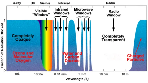
Electromagnetic radiation is made up of a continuum of wavelengths ranging from very short (gamma rays, typically 0.1 nanometres) to very long (radio waves, typically in the order of meters). The sun emits all forms of radiation within the electromagnetic spectrum (EM), but the Earth's atmosphere blocks part of the radiation and passive remote sensing (RS) from space is only possible due to atmospheric windows in different parts of the EM (Figure 2). Atmospheric windows are parts of the EM where the atmosphere has a small influence on the transmission of light and determine which wavebands are available for oceanography. For instance, in the visible region (400-700 nm), atmospheric opacity is low allowing for the analysis of the “colour” of the targets observed. In fact, the visible portion of the EM accounts for approximately 45 % of total solar energy (Kirk, 1994) and, as a consequence, evolution has resulted in many organisms
34
utilising the visible portion of the EM whether for sight, as with the case of humans, or for energy, as in the case of photosynthetic organisms (Falkowski and Raven, 1997).
Figure 2 Schematic representation of the atmospheric windows for remote sensing.
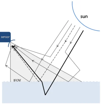
Ocean colour satellites orbit the earth at around 700-800 km altitude. This means that the signal reaching the sensor needs to be corrected for the atmospheric component. More than 90 % of the signal reaching the sensor has an atmospheric origin, which needs to be subtracted from the total signal in order to get only the portion coming from the target of interest, in this case, the ocean. This means that only ~10 % of the signal reaching the sensor is relevant to retrieve the optically active sea-water components (Figure 3).
35
Figure 3 Schematics of light pathways reaching a remote sensor (adapted from IOCCG, 2000). IFOV refers
to the instant field of view of the sensor.
Different atmospheric correction procedures have been developed to retrieve the ocean-colour signal (e.g. Gordon, 1997). The most simple correction relies on the fact that the water absorbs all radiance in the near infra-red (NIR) part of the spectrum (i.e., zero reflectance), which is also known as the “black pixel assumption” (Gordon and Wang 1994). The NIR bands are essentially used to identify the aerosol type and optical thickness in order to remove the contribution due to the atmosphere in the visible part of the spectrum (Antoine and Morel, 1999; Gordon and Wang, 1994; Siegel et al 2000). Once the upwelling radiance coming from the sea surface has been isolated, it can be used to infer on the water components. This involves the analysis of variations in magnitude and spectral quality of the water-leaving radiation to derive quantitative information on the type of substances present in the water and their concentrations. In other words, involves the analysis of the optical properties that characterize a water body, which contain latent information on its optically active constituents (OACs). Preisendorfer (1961) defines these optical properties according to their invariance under changes in the incident radiance distribution about the point at which the property is measured. According to this author, if the property is invariant with respect to changes in the radiance distribution, it is said
36
to be an inherent optical property, otherwise it is an apparent optical property. It should be noticed that all optical properties of ocean waters are wavelength (λ) dependent (IOCCG, 2000).
1.1.1.1 Apparent optical properties (AOPs)
Apparent optical properties (AOPs) are those optical properties that are influenced by the angular distribution of the light field, as well as by the nature and quantity of substances present in the medium (IOCCG, 2000). That is, properties which can be modified by the zenith-angular structure of the incident light field. Typically include the normalized water leaving radiance (nLw(λ)), the remote sensing reflectance (Rrs(λ)) and the downwelling diffuse attenuation coefficient (Kd(λ)).
Radiance L(λ) is defined as the measure of light energy leaving an extended source (Robinson, 2004) and depends on both the viewing and illumination geometry. It is a measure of radiant flux per unit area and per unit solid angle. Water leaving radiance (Lw(λ)) is the measure of the component of light energy leaving the water. The normalized water-leaving radiance (nLw(λ)) is its normalization to a single sun-viewing geometry (Gordon, 2005): i.e., the radiance that would be measured leaving the flat surface of the ocean, with the atmosphere absent and the sun directly overhead (i.e. at zenith).
The ratio of upwelling and downwelling irradiances (Eu(λ) and Ed(λ), respectively) is defined as
reflectance. Irradiance being the radiant flux per unit surface area in all directions. Reflectance is therefore a measure of how much of the downwelling light is reflected back up (Robinson, 2004). In ocean colour, remote sensing reflectance (Rrs(λ)) is commonlly defined as the ratio of the upward normalized water leaving radiance (nLw(λ)) and the downwelling irradiance (Ed(λ)).
The downwelling diffuse attenuation coefficient, KEd(λ), defines the rate of decrease of
downwelling irradiance with depth. That is, the variation of downwelling irradiance (Ed(λ)) in the
water column per depth unit. It can be expressed according to dEd(λ ,z)/Ed(λ ,z) = -Kd(λ )dz, where z is depth in metres. It is one of the geophysical variables that can be derived from ocean-colour
data, and is often used as an index of water clarity.
These apparent optical properties are quantities measurable by remote sensing, but the ultimate goal is to derived, from them, quantitative information on the types of substances present in the water and on their concentrations. It is then necessary to relate the apparent optical properties to the substances in the water and its inherent optical properties.
37 1.1.1.2 Inherent optical properties (IOPs)
Inherent optical properties (lOPs) are independent of variations in the angular distribution of the incident light field, and are solely determined by the type and concentration of substances present in the medium (Preisendorfer, 1976 in IOCCG, 2000). This typically relates to how the water constituents present in the medium, absorb and scatter light. The IOPs can therefore be defined as those describing the probability of photon removal and photon redirection per unit length. The fundamental IOPs are the absorption, scattering and beam attenuation coefficients (a, b and c, respectively), where c=a+b, and the volume scattering function, which describes the scattering relative to the direction of light propagation and azimuth angle. Measurements of the volume scattering function are not commonly performed and restricted in the field to scattering coefficients.
An important characteristic of IOPs is that they are additive. This means that, for a seawater sample containing a mixture of constituents, the absorption and scattering coefficients of the various constituents are independent, and the total coefficient can be determined by summation. In an aquatic medium, the bulk IOPs are the sum of the IOPs for water itself and all the solutes and particles contained in it. Because of the impossibility of measuring the IOPs of each individual constituent, components are grouped operationally based on their spectral similarity or defined analytically. For total a(λ), for example, Prieur and Sathyendranath 1981, suggested partitioning into contributions from: (1) water (aw(λ)), (2) coloured dissolved organic
matter, CDOM (acdom(λ)), (3) phytoplankton (aphy(λ)) and (4) non-algal particles, NAP (aNAP (λ)) (i.e.
atotal=aw+aCDOM+aphy+aNAP). The same consideration can be applied to scattering (i.e.
btotal=bw+bNAP+bphy), but note that there is no scattering by CDOM. All these coefficients are bulk
inherent optical properties, whereby each constituent in the water column is considered as a composite entity with no regard as to specific component contributions. The contributions of each component can be expressed as the product of the concentration of that substance and a corresponding specific absorption coefficient. The specific coefficient is the absorption normalized by the concentration of the constituent of interest (e.g. a*phy(λ)=aphy(λ)/Chl). The
absorption coefficients superscripted by an asterisk indicate the absorption components of each constituent per unit concentration. Analog for scattering.
Other IOPs can be derived given the mentioned basic set. For example, back-scattering coefficient (bb) is defined as the integral of the volume scattering function (β(χ)) over all
38
backward directions χ>90. From an Earth observation perspective, the bulk backscattering coefficient (bb) from the ocean may be attributed mainly to bubbles, submicron particles and
viruses (Stramski and Kiefer, 1991; Zhang et al., 1998), and some larger particles. Phytoplankton groups such as Coccolithophores and Trichodesmium can also have a particularly strong influence on backscattering of light (Balch et al, 1996; Subramaniam et al., 2002). Absorption, however, has been found to be the main optical property that can be used to identify phytoplankton (Ciotti et al., 2002), as phytoplankton absorb light for photosynthesis.
1.1.2 Water types
Based on their optical properties, water types/classes have been defined to simplify algorithm development. Case 1 waters were identified by Morel and Prieur (1977) and Gordon and Morel (1983) as waters for which phytoplankton and their associated materials (such as debris, heterotrophic organisms and bacteria, excreted organic matter) control the optical properties. Using Chl as a proxy for phytoplankton, it can be said that the Chl concentration defines the optical properties of Case 1 waters, which denotes not only Chl a pigment per se but also includes divinyl Chl a and chlorophyllide a, when the pigments are determined via high performance liquid chromatography (HPLC) technique (Morel and Antoine, 2011). However, this dependence of optical properties on Chl is not linear, the main reasons being: (1) the varying detritus-to-Chl ratio; (2) the varying pigments-to-Chl ratio in algal cells; (3) the packaging effect, which is an internal “shadowing” effect of the pigment that occurs in bigger cells with high pigment content; (4) the relative proportions of algae and of endogenous "yellow substance" which are not regularly varying along with Chl; to name a few (Morel and Antoine, 2011). Despite the non-linearity, optical properties follow closely the optical properties of phytoplankton. However, in regions influenced by land drainage or by sediment resuspension, the optical properties depart from those in Case 1 waters because of the presence of at least two additional components, already mentioned in the previous section, which can occur separately or simultaneously and are not generally correlated with Chl, namely: (1) the coloured dissolved organic matters, collectively named "yellow substance", or CDOM; and (2) the mineral particles and various suspended sediments also referred to as non-algal particles (NAP). Generically, the optical properties of a “natural” water body are dependent on the presence/variability of these three OACs (phytoplankton, CDOM and suspended sediments) Figure 4. In other words, the presence and varying proportion of these components strongly change the optical properties of a water body.
39
Figure 4 Factors that influence the upwelling light leaving the sea surface (adapted from IOCCG, 2000). Y -
yellow substance (or CDOM); S – suspended sediment (or NAP); P – phytoplankton. IFOV refers to the sensors instant field of view.
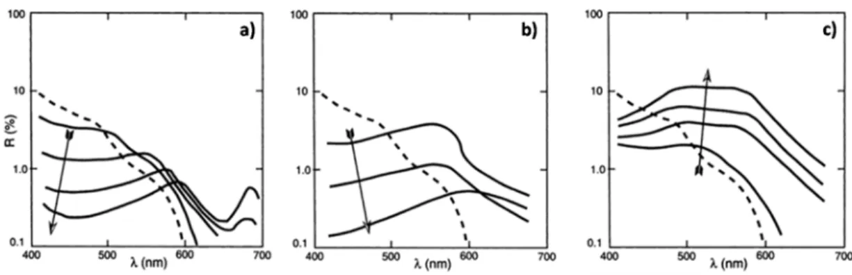
For instance, the yellow substance-dominated waters are essentially absorbing (thus with extremely low reflectances), whereas the sediment-dominated waters are strongly scattering, with high reflectances (Figure 5).
40
Figure 5 Reflectance spectra of water masses dominated by different optical active components.
Chorophyll (a), Yellow substance (b), and Inorganic sediments (c). Arrows indicate increasing concentration. (Image taken from Robinson, 2004)
It is generally recognized that Case 2 waters are more complex than Case 1 waters in their composition and optical properties. Interpretation of an optical signal from Case 2 waters can therefore be rather difficult. The "natural" waters have been conceptually organized by Prieur and Sathyendranath (1981) in Case 1 and Case 2 according to the triangular diagram in Figure 6. The 3 tips (denoted Chl, Y and S) represent the Chl-dominated waters, (i.e. the "true Case 1 waters"), the yellow substance-dominated Case 2 waters, and the sediment dominated Case 2 waters, respectively. The central part of the triangle represents Case 2 waters with various mixtures of OACs.
In Case 1 waters, and depending on the trophic regime, the Chl concentration can vary over about 3 orders of magnitude, starting from very low values (~0.02 mg m-3) in vast oligotrophic
zones (as subtropical gyres) up to high values, 5-30 mg m-3, in more restricted upwelling areas
(e.g. off Peru, Mauritania or Benguela), or during the short blooming period in moderate and high latitude ocean, as observed off the coast of Portugal.
41
Figure 6 Water type classification scheme (in Morel and Antoine, 2011) Y - yellow susbstance; S –
suspended sediment; Chl - phytoplankton
Geographically, Case 2 waters are usually associated to coastal zones, where the presence of rivers and dynamic processes like waves and tides promote introduction and resuspension of sediments. Contrastingly, Case 1 waters are typically associated to the open ocean, which does not mean that such waters are uniform. Peculiar situations are to be expected in the open ocean like the occurrence of monospecif blooms such as coccolithophorids blooms (Brown and Podestá, 1997), Trichodesmium blooms (Subramanian et al., 1999), Phaeocystis, or
Synechococcus blooms (Morel, 1997), which lead to strong deviations from the Case 1 typical
properties. In fact, the association of coastal an open ocean waters to Case 2 and Case 1 waters, respectively, can be misleading as waters can be differently classified depending on criterion applied (Mobley et al., 2004) and non-Case 1 waters can be found offshore (Lee and Hu, 2006).
42
1.1.3 Ocean colour algorithms
Satellite sensors cannot measure lOPs of the sea directly, instead they measure AOPs. In order to determine lOPs they must be estimated from AOPs, which implies assumptions on the distribution of the underwater light field. An unique expression, namely the radiative transfer equation (RTE), establishes the exact relationship that links the two classes of properties. Deriving the AOPs from the knowledge of IOPs combined with boundary conditions (e.g. the incident solar radiation) is generally called the forward problem; the inverse problem consisting of retrieval of the IOPs from measured AOPs under known illumination conditions. However, both problems require the manipulation of the RTE, which are integral equations that do not permit an easy solution. This has resulted in the development of a variety of numerical and analytical techniques involving approximations in order to produce a solution (Robinson, 2004). Empirical, semi-empirical and analytical techniques have arisen that directly estimate lOPs and/or water substances concentrations from AOPs using satellite data (see Carder et al., 1999; Garver and Siegel, 1997; Lee et al., 2002; Maritorena et al., 2002; O’Reilly et al., 1998; Smyth et al., 2005).
Empirical approaches rely on a specific spectral feature, such as a spectral ratio modelled to biophysical measurements using statistical regression, whereas semi-analytical algorithms rely on greater knowledge of optical properties of the water column and dealing to isolate the spectral influence of several optical variables (IOCCG, 2006). The empirical algorithms are derived from regression of coincident ship and satellite observations of Lw(λ) against shipboard observations of Chl. The inputs to these algorithms are satellite observations of Lw or equivalently Rrs at several wavelengths; the output is Chl concentration.
Chlorophyll a absorbs light in the blue and red portions of the visible spectrum and reflects light at green wavelengths (Figure 5-a). As the Chl concentration increases, light is absorbed more strongly in the blue and red portions of the spectrum and reflects more strongly in the green. Therefore, as Chl increases, the reflectance in the blue regions decreases and in the green it increases slightly. Thus a ratio of blue to green water reflectance can be used to derive quantitative estimates of the satellite-derived Chl concentration. However, one has to be cautious when using band-ratio algorithms to derive the Chl concentration as they will only function in waters whose variations in optical properties are mainly driven by the abundance of phytoplankton, i.e. Case 1 waters. In more optically complex waters (Case 2 waters), where Rrs(λ) is more heavily influenced by CDOM and suspended sediments, band ratio algorithms are likely to break down. Various authors have attempted to used semi-analytical models to derive
43
the Chl concentration in more optically complex waters (e.g. Morel and Maritorena 2001; Maritorena et al., 2002).
Operational algorithms in use by Space Agencies for Chl products retrieval are generally band-ratio algorithms derived and applicable to Case 1-waters, although specific algorithms have been also developed for application in Case 2-waters (e.g. Algal 2 MERIS product, Doerffer and Schiller, 2007). Chlorophyll is typically the main variable derived from ocean colour imagery and its synoptic estimates have allowed to greatly increase the knowledge about spatial, seasonal and inter-annual variability of phytoplankton biomass as indexed by Chl, at regional and global scales (e.g. Behrenfeld et al., 2006; Dandonneau et al., 2004; Kahru and Mitchell, 1999; Kahru et al., 2012; Werdell et al., 2009; Yoder et al., 2010).
1.1.4 Ocean colour sensors
The first ocean colour dedicated mission was the NASA’s proof-of-concept sensor, Coastal Zone Color Scanner (CZCS), which exceeded all expectations and end up operating from 1978 until 1986. CZCS was aboard satellite Nimbus 7 wich was launched into a 995 km near polar sun-synchronous orbit in 1972 (Gibson et al., 2000). The CZCS obtained reflected radiation in five bands in the 433-800 nm range and had a spatial resolution of 825 m for a 1,556 km wide swath (Gibson et al, 2000). With the goal of measuring water-leaving radiance, at a limited number of wavebands in the visible domain, and to use the signal to infer concentrations of phytoplankton pigments in the near-surface layers of the ocean, CZCS demonstrated, for the first time, the feasibility of retrieving Chl from RS data on a synoptic and global scale. The next satellite instruments were the Japanese Ocean Colour and Temperature Sensor (OCTS) on the ADEOS-1 satellite that operated from August 1996 to June 1997, and the German Modular Optical Scanner (MOS) launched in 1996 on the Indian Remote Sensing Satellite IRS-P3 (Martin, 2004). The Sea-viewing Wide Field-of-view Sensor (SeaWiFS) was launched on the ORBVIEW-2 satellite in August 1997, and operated between the 412-865 nm range since September 1997 until December 2010. The Moderate Resolution Imaging Spectrometer (MODIS) was launched on the TERRA satellite in December 1999 and on AQUA satellite in May 2002 (Martin, 2004). MODIS sensors have a spatial resolution of 250 m in the UV band, 500 m in the visible waveband in the red, and 1 km in the ocean-colour wavebands (Robinson, 2004). In March 2002, the European Space Agency (ESA) launched its first ocean colour sensor, the Medium Resolution Imaging Spectrometer (MERIS), onboard the ENVISAT platform, where MERIS is in a descending
sun-44
synchronous orbit with 15 observing bands between 400 and 900 nm (Martin, 2004). Its primary goal was to monitor ocean colour. However, it was also designed to determine atmospheric and land surface information. MERIS had five parallel arrays to gain a swath width of 1150 m, offering ocean colour and geophysical products at a reduced resolution of 1200 m (RR) and full resolution (FR) capability of 300 m (Robinson, 2004). MERIS operationally ceased in April 2013. More recently (March 2011), NASA launched the Visible Infrared Imaging Spectro-Radiometer Suite (VIIRS), under the National Polar-orbiting Operational Environment Satellite System (NPOESS). ESAs next ocean colour mission is expected to be launched in 2014, Ocean and Land Colour Instrument sensor (OLCI) on Sentinel-3 satellite, within the European Union-ESA Global Monitoring for Environment and Security (GMES) programme.
Table I List of ocean colour sensors (IOCCG, 2012)
Sensor (Satellite) Mission Developer Launch year Resolution Spatial (m)
CZCS (NIMBUS-7) NASA (USA) 1978 825
POLDER (ADEOS) CNES (FRANCE) 1996 6000
OCTS (ADEOS) JAXA (JAPAN) 1996 700
SeaWiFS (SeaStar) NASA (USA) 1997 1100
OCI (ROCSAT) NSPO (TAIWAN) 1999 800
OCM (IRS-P4) ISRO (INDIA) 1999 350
MODIS (Terra/Aqua) NASA (USA) 1999 1000
MERIS (ENVISAT) ESA (EU) 2002 300 & 1200
GLI (ADEOS-II) JAXA (JAPAN) 2002 1000
COCTS (HY-1B) CAST (CHINA) 2007 1100
GOCI-I (COMS) KIOST (KOREA) 2010 500
VIIRS (Suomi NPP) NOAA (USA) 2011 750
OLCI (SENTINEL 3) ESA (EU) 2014 300
SGLI (GCOM-C1)
JAXA (JAPAN) 2015 250 & 1000
GOCI-II
(GeoKOMPSAT-2B)
45
1.1.5 Ocean colour products validation
Ocean-colour missions have revealed the importance of validating satellite products. NASA (e.g. SeaWiFS, MODIS) and ESA (e.g. MERIS) sensors have been validated with both geographically distributed field measurements and radiometric data collected by moored systems. The space agencies defined as goals for accuracy 5% for radiometry and 35% for Chl concentration (e.g. McClain, 2009) supporting large datasets programs for algorithm development and validation (e.g. NASAs SeaBASS database and ESAs MERMAID matchup database). Although global results are within the error expectations, satellite validation with in situ data has revealed the need for specific algorithm adjustments at regional levels (e.g. Folkestad et al., 2007; Garcia et al., 2005; Komich et al., 2009; Ohde et al., 2007; Sorensen et al., 2007; Volpe et al., 2007).
The need for validation of ocean-colour products is also emphasized by the necessity of merging satellite ocean colour observations. Different projects have focused on data merging to provide continous global products, including the GlobColour project (http://www.globcolour.info), the NASA SIMBIOS Program (McClain et al., 2002; Maritorena and Siegel, 2005), and the recent OC-CCI ESA project (Ocean Colour Climate Change Initiative). Such projects aim to improve the consistency of ocean colour time-series, spatial and temporal coverages, and produce the necessary requirements to use ocean colour as an Essential Climate Variable (EVC). This thesis uses the MODIS and MERIS datasets for ocean colour product validation off the Portuguese coast.
1.2 Phytoplankton
The term plankton was introduced by Viktor Hensen in 1887, and originally described “everything that drifts in the water, whether shallow or deep, living or dead” (from Taylor 1980
in Hoppenrath, 2009). The term evolved to include only living organisms caused probably by the
“Plankton-Studien” of Ernst Haeckel published in 1890 (Taylor 1980 in Hoppenrath, 2009). Phytoplankton refers to the phyto, “plants” in greek, component of plankton. The small “plants”/ “algae” / photosynthetic protists that drift in the water column. A broad variety of taxa are represented in the marine phytoplankton, including cyanobacteria, Prochlorophyta, Chlorophyta, Euglenophyta, Dinophyta, Cryptophyta and Chromophyta (Bacillariophyta, Chrysophyceae, Rapidophyceae and Prymnesiophyceae). These phytoplankton communities are essential to the majority of ecological processes and affect the structure of food webs (e.g., primary production), nutrient cycling and the flux of particles to deep waters. Primary production is one of the most important ecological aspects of the phytoplankton as the biomass
46
built through photosynthesis is the nutritional basis for all higher trophic levels (e.g zooplankton). Revelance of phytoplankton role not only in the oceans but also in the global ecosystem has been emphasized by Field et al (1998) remote sensing study, where, for the first time, estimates of phytoplankton production were shown to account for 50 % of the worlds primary production.
Phytoplankton distribution changes both horizontally and vertically (Barlow et al., 2007; Brunet and Lizon, 2003; Leal et al., 2009). Locally, temperature, salinity and currents, along with other factors, determine the horizontal distribution, while vertical distribution is primarily determined by irradiance, nutrients and water column stability. The effect of these factors on phytoplankton abundance and community structure is known to vary among worldwide regions, from tropical to temperate ecosystems (Longhurst, 1998).
1.2.1 Phytoplankton: size classes and functional types
Phytoplankton cover a wide spectrum of biological diversity (Bowler et al., 2009), encompassing taxonomic groups with distinct sizes, life cycles, turn-over rates, nutrient stoichiometry, biochemical composition and ecological requirements, performing therefore an array of diverse functions in the marine ecosystem. In this context, phytoplankton functional types (PFTs) have been defined to link certain phytoplankton groups (which can be polyphyletic) with specific biogeochemical functions (Nair et al., 2008). The number of defined PFTs can vary according to the scientific question being addressed (Le Quéré et al., 2005), but calcifiers (coccolithophores), silicifiers (diatoms), nitrogen fixers (Trichodesmium and N2 fixing prokaryotes), pico-autotrophs
(pico-eukaryotes, and cyanobacteria such as Prochlorococcus and Synechococcus) and DMS producers (e.g., autotrophic flagellates) are commonly considered.
Concerning size, phytoplankton have been categorized in: (1) picoplankton (<2 µm in diameter), comprising pro-prokaryotes (cyanobacteria, prochlorophytes and other bacteria) and pico-eukaryotes; (2) nanoplankton (2-20 µm), eukaryotic flagellates (cryptophytes, chrysophytes, prymnesiophytes and chlorophytes); (3) microplankton (20-200 µm), diatoms and dinoflagellates (Sieburth et al., 1978). This size-based approach to phytoplankton functionality is not always fully satisfactory from a biogeochemical perspective (Nair et al., 2008). For example, diatoms are silicifiers and typically categorised as micro-phytoplankton, yet some diatoms fall into the nano-size range. Although these smaller diatoms have the same biogeochemical function, they are likely to respond differently with respect to size-based functionality (e.g., export production).
47
There are also some examples of nano-phytoplankton of a similar size having a contrasting biogeochemical function (e.g., calcifiers and DMS producers). Despite this, many functions of phytoplankton, such as nutrient uptake, light absorption, metabolic rates and sinking are strongly related to size.
1.2.2 Phytoplankton Pigments
Phytoplankton contain three types of pigments involved in light harvesting and photoprotection: chlorophylls, carotenoids and biliproteins (Wright and Jeffrey 2006). All photosynthetic phytoplankton contain one or more types of chlorophylls as part of the light-harvesting complexes in their chloroplasts. Chlorophyll a (Chl) is ubiquitous to phytoplankton and the reason why it is used as a biomass proxy. Chlorophyll a are magnesium coordination complexes of conjugated cyclic tetrapyrroles with a fifth isocyclic ring and often esterified long-chain alcohol (Figure 7). Other chlorophylls differ according to the oxidation state of the macrocycle, the type of side-chains, and the type of esterifying alcohol, if present. For instance, Divinyl form of Chl, which can be found in prochlorophytes, results from a substitution of an ethyl group into a second vinyl one.