Equity Valuation – EDP Renováveis
Frederico Ladeira Teixeira Dias I 152413015 Advisor: José Carlos Tudela Martins
Master Thesis I MSc in Finance
January 2015
Dissertation submitted in partial fulfilment of requirements for the degree of MSc in Finance at Universidade Católica Portuguesa
Abstract
The renewables industry has been facing an important diffusion in the world of long-term energy scenarios. The necessary strict control over carbon dioxide emissions and the diversification of energy sources through ambitious world commitments is leading to a promising and continuously development of this sector.
The equity valuation exercise here proposed aims to explore the connection between theoretically fundamentals with the practitioners work basis.
We have designed a well theoretically supported work, with a cautious literature revision, and strongly adjusted for what equity research industry defends in practice, trying to deeply explore a more robust valuation exercise.
EDP Renováveis (EDPR) is considered to be one of the leading players in the wind industry and its valuation requires a thorough analysis of industry and company specifications, considering also the actual financial markets conditions.
This dissertation foresees a future development path of EDPR, based on its current framework, investment plan and natural redirections of its growth, as it has been assisted in the entire industry.
We forecast a standalone valuation for EDPR of €12.509 Billion, corresponding to a target price per share of €7.10.
Nevertheless, the consistent uncertainty of few main drivers’ comportments and whole projects construction, a sensitivity analysis is computed in order to account the potential future of this company.
Independently of the sensitivity results of the base case, this equity valuation exercise clearly indicates a BUY recommendation.
Acknowledgments
The Master of Science in Finance at Católica Lisbon School of Economics was one of the most important decisions in my life.
Its conclusion is expressed by the Master thesis that I expose here. It was possible to use the diversify knowledge obtained in the masters’ courses that allow me to face this practical case, an equity valuation, with strong theoretically and practice fundamentals.
The Equity Valuation Seminar was the perfect framework to develop this dissertation, being mandatory to express my gratitude to Professor José Carlos Tudela Martins, for his availability and help in several questions that I raised during this last 4 months, always complementing with trustful and important comments; but also to express thanks to my seminar colleagues, given the questions and topics discussed during and outside the seminar sessions.
I would also to express my thanks to Dr. Luís Guimarães for its technical support, but also for all valuable insights and discussions that we had, representing a crucial help for this work. Finally, I would like to remark a set of people who are indispensable for me, in this specific time of my life.
I would like to express my gratitude to Ana Azevedo Branco, Tiago Lopes Sequeira and Francisco Varandas Fernandes, for their distinctive support, personally and technically speaking, being impossible to finish this dissertation without them.
With the same feeling, I would like to especially thank to my parents and my sister, and finally to my old friends, namely Pedro Guimarães, Gonçalo Morgado, Diogo Portinha e Luís Oliveira, for providing me incentive words, and all necessary support to perform this stage successfully.
This dissertation represents simultaneously the end of an important academic path and the beginning of my professional life, which I will face optimistically.
Index Introduction ...9 1. Literature Review ... 10 1.1. Equity Valuation... 10 1.2. Relative Valuation ... 11 1.2.1. Multiples Analysis ... 11 1.2.2. Peer Group ... 12
1.3. Discounted cash-flow methods ... 12
1.3.1. Terminal Value ... 14
1.3.2. Discount rate ... 16
1.3.3. Weighted Average Cost of Capital ... 17
1.3.4. Capital Asset Pricing Model ... 17
1.3.5. Adjusted Present Value ... 20
1.3.6. Dividend Discount Model ... 23
1.4. Profitability models ... 24
1.4.1. Economic Value Added (EVA)... 24
1.4.2. Residual Income (RI) or Dynamic ROE... 24
1.5. Option Pricing Theory... 25
1.6. Note of cross-border valuation ... 26
1.7. Note of valuation of Utilities ... 27
1.8. EDPR – Theoretical assumptions ... 27
2. Industry and market review ... 29
2.1. Renewable Energy Industry ... 29
2.2. Wind Energy Industry ... 32
2.2.1. World portfolio – Re-shifting of installed capacity ... 32
2.2.2. “Are renewables energies a luxury?” – Cost competitiveness ... 35
2.2.3. Regulatory systems ... 37
2.3. Macroeconomic Framework ... 39
2.4. Company Overview ... 40
2.4.1. Shareholder structure and share performance ... 40
2.4.2. The top quality portfolio... 42
2.4.3. Asset rotation strategy ... 46
2.4.4. EDPR - National markets & regulatory framework... 47
2.4.6. Portugal ... 49
2.4.7. Rest of Europe ... 50
2.4.8. North America: US, Canada and Mexico ... 51
2.4.9. Brazil... 53
2.4.10. Offshore ... 54
2.5. Business risks and opportunities ... 54
3. Valuation ... 56
3.1. Projections ... 56
3.1.1. Portfolio Expansion Program ... 57
3.1.2. Projected Revenues ... 57
3.1.3. Projected Operating Costs ... 59
3.1.4. Provisions... 59
3.1.5. Depreciation, Amortization and Government Grants... 60
3.1.6. Capex ... 60
3.1.7. Investment in Net Working Capital... 61
3.1.8. Tax Rate ... 62
3.1.9. Explicit Period and Terminal Value ... 62
3.1.10. Cost of Capital – Unlevered Cost of Equity ... 63
3.2. Financing Plan – Market Value of Debt and Interest Tax Shields ... 64
3.3. Results of the valuation exercise ... 66
3.3.1. EDPR APV valuation ... 67
3.3.2. Relative Valuation – Market Multiples Analysis... 69
3.3.3. Comparison exercise – Millennium Investment Banking (MIB) Equity Research Note . 70 3.3.4. Sensitivity Analysis ... 71
Conclusion... 74
Appendix ... 76
Bibliography ... 87
Index of Figures
Figure 1: World Energy Drivers
Figure 2: Worldwide and Renewable Additions Figure 3: World Wind Capacity 2011-2014 (MW) Figure 4: LCOE of Wind industry derivation Figure 5: Capex Wind Onshore breakdown
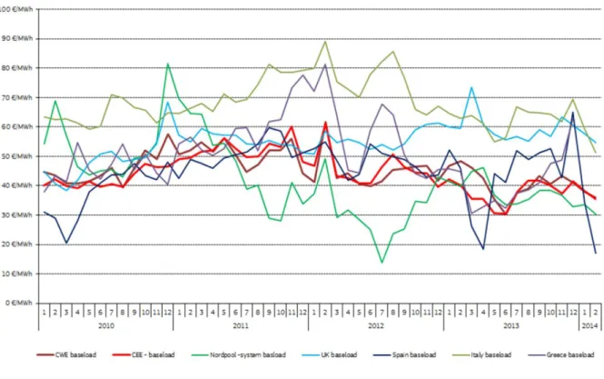
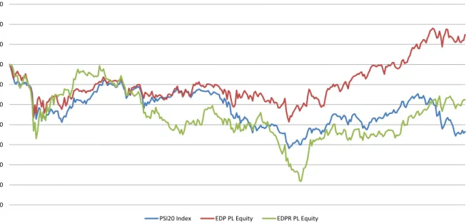
Figure 6: Wholesale Electricity Prices in Europe (€/MWh) 2010-2014 Figure 7: Stock performance over the period 2008-2014
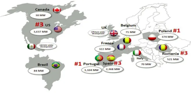
Figure 8: EDPR’s Portfolio September 2014
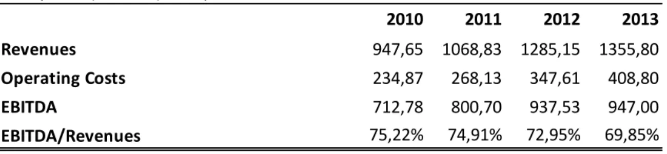
Figure 9: Revenues, Operating Costs and EBITDA Margins
Figure 10: NOPLAT and ROIC evolution over the period 2010-2013 Figure 11: MW capacity over the period 2014-2039
Figure 12: Remuneration Scheme and 2014 prices
Figure 13: Revenues and Operating Costs over the period 2014-2039 (€Million) Figure 14: Capex Estimations
Figure 15: Calculation of Beta Figure 16: Unlevered Cost of Equity
Figure 17: EDPR's debt plan (€Million) over the period 2014-2039 Figure 18: EV breakdown (€Million)
Figure 19: From EV to Equity Value (€Million) Figure 20: Relative Valuation
List of abbreviations
ANEEL National agency of electric energy BNDES Banco Nacional do Desenvolvimento
FiT Feed in Tariff GW Gigawatt
IPO Initial Public Offering IRR Internal Rate of Return MW Megawatt
NA North America
O&M Operating and Maintenance P.P. Percentage points
PPA Purchase Power Agreements
PROINFA Program of incentive to the electric energy alternative sources
Q&A Questions and Answers
REC Renewable Energy Certificates ROC Renewable Obligation Certificates
RoE Rest of Europe
SG&A Selling, General and Administrative expenses Solar PV Solar Photovoltaic
UK United Kingdom
US United States of America YoY Year Over Year
Introduction
The present dissertation has the purpose of presenting a trustable and professional valuation exercise of EDPR. The main objective is so to estimate a value for EDPR’s stock based on its particular fundamentals. EDPR is a leading company in renewable energy industry highly supported by its integration in EDP Group (EDP), listed on Euronext Lisbon since 2008.
This dissertation answers simultaneously to different motivations. Firstly, it is desired that it provides a superior understanding of equity valuation methodologies, combining the theoretically and practice principles. Secondly, the aim of exploring a complex and interesting industry, essentially given its financial and technological oriented structure, and finally, the opportunity to place in practice the knowledge that acquired during the Master of Science in Finance.
This work is so organized in three major sections, beginning with the literature review, passing through the industry and company overview and concluding with the valuation section.
The literature review is a crucial section, exploring the state of the art, which will be the theoretically support of the dissertation. The company and industry overview develops the framework in which EDPR is inserted, underlying relevant topics to be accounted when the valuation is performed. It gives a general picture of the company today’s situation, adding an important valuable analysis to understand, even superficially in some topics, the renewable energy industry. Lastly, the valuation section displays our methodology and results, explaining in detail the main assumptions behind the valuation model with a specific comparison exercise, concluding with an estimation of 2014 target price for EDPR stock. In sum, our work designs a robust and coherent path of valuation analysis, combining the different school of thoughts with the fundamentals of the industry and the proper specifications of EDPR. The final result is an investment recommendation, a specific output that nowadays has significant relevance on investors’ decisions and capital applications.
1. Literature Review
In this first section of this dissertation, it is summarized the state of the art, analyzing the existent set of models to perform a valuation exercise of a company.
Each model will be defined and explained, emphasizing the literature developed about them, their fundamentals, strengths and weaknesses, and their final results.
It is important to notice that some details regarding the valuation models are only presented in valuation section, where the company’s characteristics are discussed and adjusted to the methodologies explained previously.
After this discussion, there is the necessary information to design a valuation path to evaluate EDPR, selecting different methods in order to achieve stronger conclusions.
1.1. Equity Valuation
“Valuation can be considered the heart of finance.”1.
The valuation process is a complex but useful exercise, designed individually for each company. Several academics and professionals have been focused on this process, specifically on the choice of the right valuation models, taking into consideration the different drivers from the different businesses areas and industries.
The different valuation models contribute individually to the big picture. Looking at it, it is possible to understand why different results are achieved over the models, and which assumptions do not make sense, accurate the global valuation exercise.
According to Fernandez (2013), the mechanism of companies’ valuation is a critical point in the corporate finance domain, which has been developed by equity researchers and investors. More, it is also an important concept for the managers’ day-by-day by identifying sources of value creation through valuation of the company and its different business units.
1
Damodaran, Aswath. “Valuation approaches and metrics: A survey of the theory and evidence”. Now Publishers Inc, 2005
Damodaran (2005) indicates that in order to make reasonable and sensible valuation decisions, it is mandatory to understand what determines and influences the firm’s value, and how the best way to estimate it.
According to the author, there are four main approaches to valuation: relative valuation, discounted cash flow valuation, contingent claim valuation and liquidation and ac counting valuation. In this work, it will be explored the first three approaches, once the last one is considered only for liquidation or short-term “fire sale” purposes.
1.2. Relative Valuation 1.2.1. Multiples Analysis
The valuation using multiples is one of the most popular valuation methods among financial analysts, researchers and investors, as it is reported in Asquith et al (2005) “(…) 99% of top analysts use a multiplier model for firm valuation”.
“Valuation by multiples entails calculating particular multiples for a benchmark companies and then finding the implied value of the company of interest based on the benchmark multiples” is stated in Lie and Lie (2002) as a definition of the model.
In Lie et al (2001), this method is appointed as a method which facilitates the comprehension of other valuations, once communicates clearly the end result of those valuations. More, they argued that a valuation using multiples complements other valuations by calibrating their final results and helping to obtain the terminal value.
As we stressed previously, the relative valuation has two main critical points: to choose which multiples to use and the peer group selection. These critical points are considered the main drivers of the valuation and the output can vary significantly if we apply different drivers, no matter if it is a different multiple or a different set of comparable firms.
The literature has developed the necessary requirements to build a robust and consistent analysis of comparable multiples, highlighting that the principles of valuation and the empirical evidence recommend the use of forward-looking multiples instead of using trailing multiples, once the first ones are more accurate predictors of value, as it i s reported in Liu et al (2001) and Kim and Ritter (1999).
The price-to-earnings (P/E) is a widely used multiple, even nowadays has been criticized because the distortions created by the different capital structures of the companies and the incorporation of non-operating gains and losses in final result. The enterprise value (EV) to EBITDA, a similar multiple focused in EV instead of share price, is considered and reported as the mandatory multiple when it is comparing valuations across companies. It is the multiple
that “(…) tells more about the company’s value than any other multiple.”2.
1.2.2. Peer Group
The definition of the peer group is a multifaceted and a discussed topic in literature as well. Henschke and Homburg (2009) stated that “(…) it is difficult to find a peer group which corresponds to a target firm in all value relevant characteristics”. However, to define a set of comparable firms we can use a statistical tool, the cluster analysis for exampl e, or the information that companies may disclose in their annual reports regarding their group of competitors. As it is declared in Koller et al (2005), the definition of the peers should lies on companies that have similar outlooks for return on invested capital (ROIC) and long-term growth.
Despite this method is commonly used, it is indispensable to understand the characteristics and limitations of the model in order to avoid inconsistent calculations, incoherent use of multiples and incorrect valuations, which can lead to overlook perspectives or to ignore existent risks, reason why this method is rarely used in a standalone basis.
1.3. Discounted cash-flow methods
According to Copeland et al (2000), the fact of the cash is king makes that a good valuation should be based on a Discounted Cash Flow (DCF) method. The several DCF models are reported as one of the most rigorous and secure approaches when appraising investments. These models consist in using future projections of the cash-flows of the company and discount them at an appropriate rate to obtain the present value, which allows us to evaluate a potential opportunity of investment. Furthermore, according to Ceglowski and
2
Koller, Tim, Marc Goedhart, and David Wessels. “Valuation: measuring and managing the value of companies”. Vol. 499. John Wiley and Sons, 2010.
Podgóvsky (2012), this model can be applied based on two different cash flow perspectives, the Free Cash Flow to Firm (FCFF) and the Free Cash Flow to Equity (FCFE).
The FCFF perspective refers to all resources that will be available to all financing parties, the equity and the debt holders, representing the expected cash flows from the company’s operation.
After the deduction of the taxes on earnings before interest and taxes (EBIT), it is necessary to sum up the depreciations and amortizations, previously deducted, once they are tax deductible but they represent a source of capital available for the firm. The investments done by the company are after deducted through capital expenditures (Capex) and increments on working capital (NWC), getting finally the FCFF. In order to estimate the Firm Value (FV), the FCFF must be discounted at an adequate rate, the Weighted Average Cost of Capital (WACC), a term that will be discusses further on. The FV is then given by:
𝐹𝑖𝑟𝑚 𝑉𝑎𝑙𝑢𝑒 = ∑ 𝐹𝐶𝐹𝐹𝑡 (1 + 𝑊𝐴𝐶𝐶)𝑡 𝑁
𝑡=1
The FCFE perspective refers to the amount that a firm has available to pay dividends to their equity holders, which is equal to the cash flow from operations net of all payments to debt holders.
To obtain the FCFE, the calculation process starts with the net income presented in the Profit and Losses (P&L). After, add the new debt of the company, and subtract the CAPEX and the principal repayments to debt holders. As we only are considering the resources available for shareholders, the appropriate discount rate to obtain the equity value is not the WACC, but it is the cost of equity, Re, which represents the shareholders’ opportunity cost.
𝐸𝑞𝑢𝑖𝑡𝑦 𝑉𝑎𝑙𝑢𝑒 = ∑ 𝐹𝐶𝐹𝐸𝑡 (1 + 𝑟𝑒)𝑡 𝑁
𝑡 =1
Although the two valuations are calculated differently, if the set of assumptions are specific, coherent and realistic, the final value should be the same, given the directly relation stated between the FCFF and the FCFE.
Theoretically, the application of the DCF model is not a complex process, no matters what perspective it is used. However, Pinto et al (2010) argued that if we are considering levered and non-stable capital structure firms, or companies with negative FCFE, the perspective of FCFF is more trustful with the WACC approach, regarding the sensibility of the cost of equity to the capital structure’s changes.
There are some practical questions that should be treated carefully, once the success of the valuation exercise may depend on them.
One of the most important transversal questions regarding the DCF analysis is the time frame to use in projections, or also denominated as the explicit period. The rule lies on the performing point of the company. Usually, the literature recommends an explicit period between five and ten years. However, in some cases that companies are already performing on their steady-state point, this period can be shorter, or longer, if we are considering outstanding growth companies.
The second important question is the definition of the second stage of the valuation, the terminal value. This term is an indispensable part of a DCF analysis and represents a higher proportion of the EV, reason why the methodology and concerns are discussed, later, in a specific topic.
The DCF analysis is highly influenced by the quality of assumptions for the forecasts presented, reason why it is stated that they should representing almost 80% of the time allocated to the valuation exercise and the computations only 20%. The DCF value is given so by the following equation.
𝐷𝐶𝐹 𝑉𝑎𝑙𝑢𝑒 = ∑𝐶𝑎𝑠ℎ 𝐹𝑙𝑜𝑤𝑡 (1 + 𝑟)𝑡 𝑁 𝑡=1 + 𝑇𝑒𝑟𝑚𝑖𝑛𝑎𝑙 𝑉𝑎𝑙𝑢𝑒𝑁 (1 + 𝑟)𝑁
The literature indicates the DCF model as the preferred one to evaluate companies, but also underlying that some information is distorted or is not disclosed without the use of other models, as the tax shields advantages or bankruptcy costs.
1.3.1. Terminal Value
The expected future cash flows of a company cannot be estimated forever, being impossible to have an infinite explicit period. The terminal value of a company is the denominated
second stage when valuing a company based on DCF method by Cassia et al (2007), also called the continuing value. This term quantifies the anticipated value of a company at a specific future date, after the calculation of the explicit period, by computing all projected future cash flows for a longer period.
The terminal value calculation is a critical point of every DCF analysis once it usually represents a higher percentage of the estimated EV, being influenced by the forecast horizon of the explicit period and the potential future growth of the business.
Damodaran (2012) states that there are three approaches to estimate the terminal value: the market multiples, the stable growth model and the liquidation value.
The first two approaches are the most used to estimate the terminal value and assume that the activity of the company will continue after the last year of the explicit period, on the contrary to the liquidation value.
The liquidation value assumes that the operation of the company will cease at a future certain point, and it will be liquidated. The valuation of the company is an estimation of what the market may pay for the assets that the firm has accumulated, after paying its debts. However, this model presents an approach based on the book value assets, not considering the earning power of the assets.
The multiples approach refers that the future value of the company is estimated based on the application of multiples of comparable firms on present company multiples. The rationale of this method lies on the fact that the multiples today contain the expected growth performance of the company in the future. However, there are limitations regarding this terminal value calculation, given we are mixing a discounted cash flow valuation in the explicit period with a relative valuation of the terminal value, resulting a possible non-consistent valuation.
The limitations presented above drive us to understand that “(…) the only consistent way of estimating the terminal value in a discounted cash flow model is to use either a liquidation
value or a stable growth model”3.
The stable growth model assumes that firms use part of their cash-flows to perpetual reinvest them back into new assets, increasing the life cycle of the company. As it was stressed previously, the terminal value allows us to concentrate all projected future cash flows of the company in one unique value. This reason points out the reason why when the terminal value is been calculated, the company should be in its steady-state phase, growing at a constant rate.
The terminal value calculation can be adjusted depending if we are valuing equity or valuing the firm. In both cases it is assumed a constant growth rate in perpetuity, adjusting between cash flow to equity and free cash flow to the firm, cost of equity and cost of capital, respectively. 𝑇𝑒𝑟𝑚𝑖𝑛𝑎𝑙 𝑉𝑎𝑙𝑢𝑒 𝑜𝑓 𝐸𝑞𝑢𝑖𝑡𝑦𝑡= 𝐶𝑎𝑠ℎ 𝐹𝑙𝑜𝑤 𝑡𝑜 𝐸𝑞𝑢𝑖𝑡𝑦𝑡+1 𝐶𝑜𝑠𝑡 𝑜𝑓 𝐸𝑞𝑢𝑖𝑡𝑦𝑡+1− 𝑔𝑡 𝑇𝑒𝑟𝑚𝑖𝑛𝑎𝑙 𝑉𝑎𝑙𝑢𝑒𝑡= 𝐶𝑎𝑠ℎ 𝐹𝑙𝑜𝑤𝑡+1 𝑟𝑡− 𝑔𝑡
The literature presents some concerns about this method regarding the perpetuity constant growth rate. First of all Damodaran (2005) clearly presents as impossible a firm that can grow forever at a higher rate than the growth rate of the country’s economy where it is. More, even the firm is a multi-national one, the limit of growth rate still is the growth level of the global economy. This adjustment will be crucial in the valuation section to make an accurate terminal value calculation.
1.3.2. Discount rate
In this topic it will be discussed one important part of the DCF analysis: the discount rate. The discount rate is the appropriate rate used to discount the future cash-flows considering the opportunity cost and the risk of the company, obtaining the present value of those cash
3
Damodaran, Aswath. “Investment Valuation: Tools and Techniques for Determining the Value of any Asset, University Edition”, John Wiley and Sons, 2012.
flows. The discount rate should be adjusted to the risk level of the company and also to the capital structure of the company.
1.3.3. Weighted Average Cost of Capital
The Weighted Average Cost of Capital (WACC) has been the widely discount rate used in DCF analysis. The WACC is a tax-adjusted discount rate, given the ability to incorporate the advantage of the corporate borrowing, and according to Fernandez (2010), it is a “(…)
weighted average of a cost and a required return.”4, once it contains company’s capital
structure ratios, cost of debt, cost of equity and an extra input regarding mixed instruments, as it is shown in the equation above:
𝑊𝐴𝐶𝐶 = 𝐷 𝐷 + 𝐸 + 𝑃∗ 𝑟𝑑∗ (1 − 𝑇) + 𝐸 𝐷 + 𝐸 + 𝑃∗ 𝑟𝑒+ 𝑃 𝐷 + 𝐸 + 𝑃∗ 𝑟𝑝
The limitations of this method have been discussed in the literature by several authors, considering that the WACC is the appropriate discount rate only when the capital structure of the company is relatively stable. Luerhman (1997) is one of those, stating that WACC does a poor job with companies that present complex tax structures.
As it is understood, the WACC equation has several components. Each of them is computed with specific fundamentals and models, being the most relevant the computation of the cost of equity component.
1.3.4. Capital Asset Pricing Model
To compute this component is necessary to use an asset pricing model, which allows us to yield a correct discount factor based on the level of risk of the company. The standard asset pricing model generally used is the Capital Asset Pricing Model (CAPM) introduced by Sharpe (1964). CAPM is a factor model that relates the expected required return of a security or portfolio, usually called cost of capital, with the required return appointed by the market. This model has been developed and some extensions were introduced by Fama and French (1992) and Carhart (1997), introducing factors on size and growth, and a factor over momentum, respectively.
4
Fernandez, Pablo. "WACC: Definition, Misconceptions, and Errors." Business Valuation Review 29.4 (2010): 138-144.
Despite the existence of updated and robust approaches for asset pricing models, the CAPM still is the most used model given its simplicity and its utility in companies’ valuations. The CAPM determines the expected rate of return of a security or portfolio, equals the sum of the risk free rate of the market, and the market risk premium, already adjusted to the company’s correlation with the market through the firm’s beta factor.
𝑟𝑒 = 𝑟𝑓+ 𝛽𝐿∗ [𝐸(𝑟𝑚) − 𝑟𝑓]
The risk-free rate of return is most of the times undervalued when it is accessing the expected return of the security. However, a non-careful selection of which risk free to use is sufficient to influence wrongly an entire valuation. According to Damodaran (1999), the risk free rate should be a short- or a long-term risk free rate depending of the duration of the investment analysis. More, considering the government as a default free entity, the author argues that the risk free rate used for companies’ valuations should be a long term risk-free government bond. The author points out two conditions when we are dealing with risk-free rates: the consistency principle and the inflation adjustment.
The first one lies on the fact that is the currency used to estimate the cash flows of the firm that determines the choice of the currency of the risk free rate. The second one states that the estimated cash flows and the risk free rate should be or not adjusted to the inflation, since both are in the same condition, real or nominal terms.
The risk-free component is used to compute the cost of equity but also the market risk premium and the beta of the company.
The market risk premium, also called the equity risk premium, is one of the most debated concepts in the literature, given its weight in every risk and return finance model. This term reflects the difference between the expected return on a market portfolio and the risk-free rate, combining three concepts: the required market risk premium, the historical market risk premium and the expected market risk premium.
According to Damodaran (1999), there are three main approaches for defining the market risk premium: the historical premium approach, the modified historical risk premium and the implied equity premium approach.
The standard approach is the historical premium approach that computes the market risk premium through the average of the historical differences between the market returns and the risk free returns over a long time period. Damodaran (1999) argues that this model only can be used if we are considering a mature market with historical data available, as i t is the case of the US market.
The difference to the others approaches lies on the methodology used to calculate the market data of the specific market. However, it is generally accepted as consensus by the market, investors and companies, a mature equity market risk premium between the ra nge 5% and 6%.
There are two main approaches talking about the adjustment of market risk premium for country’s risk premium or similar risks.
From Damodaran (1999) point of view, the country risk premium reflects an extra risk in a specific country, which should be added to the base premium for mature equity market. This term accounts the country’s default risk, but also many equity factors, as stability of the country’s currency or country’s politic situation, and the adjustment procedure is through the bludgeon, the beta or the market lambda approach.
The second approach states that the country risk should be directly adjusted in the cash flows, creating scenarios for the different risky situations that you could face in a specific country. To each scenario, positively and negative, it is attributed a specific probability of occurrence, leading to a resulted cash flow already adjusted.
The last factor of the equation is the beta. This factor measures the correlation between the securities’ or portfolios’ volatility with the whole market volatility. Looking to the beta, we can analyze the firm’s exposure to the market risk, which means how securities’ returns will respond to market movements.
Regarding the calculation of the beta, there are several approaches. Damodaran suggests a regression of the company’s stock returns on the market returns, paying attention to three different concepts: the market index, the frequency of the data and the time frame.
The market index used should be considered as a benchmark for the company and it should be a weighted market index. The frequency usually used by practitioners is weekly or
monthly returns, once daily returns are negatively correlated even a higher frequency allows more observations. The time frame is a tricky concern once on one hand with a higher time frame we obtain more observations and so a stronger regression, on the other hand, the characteristics of the company may be different along this time frame and the regression will be biased. The following relationship permits us to estimate the beta levered for the company.
𝑟𝑖 = 𝛼 + 𝛽 ∗ 𝑟𝑚
The beta term has a directly relation with the leverage level of the company. The incremental risk in case of the company has debt is reflected directly in the unlevered beta of the company, arising it. Through the Damodaran suggestion, the obtained beta after the regression is the levered beta of the company, and consequently, to obtain the unlevered beta for the CAPM calculation of the cost of equity, it is needed to rearrange this equation to do so.
𝛽𝐿= 𝛽𝑈∗ [1 + (1 − 𝑡) ∗ 𝐷 𝐸]
The second strategy also explained by Damodaran to estimate the unlevered beta of a
specific company is the bottom-up strategy5. This strategy is driven by a peer group, which
should be diversified as possible inside the industry segment, once it is able to capture all effects of the industry risks overall the world, assessing a better unlevered beta. After the deleveraging of the betas of the peer group, it is computed the average of unlevered betas, further leverage adjusted to the financial profile of the company, getting the company’s specific levered beta.
1.3.5. Adjusted Present Value
The Adjusted Present Value (APV) model appears as the preferred model to use in substitution of the DCF/WACC model, regarding the limitations already discussed.
The APV valuation model calculates the value of the company as if it is solely equity financed, adding the financing benefits in a second stage of the valuation exercise taking into consideration the bankruptcy costs. Indeed, APV provides important information for
5
management teams, making possible to analyze the contribution of each of source of value to the company’s present value.
Moreover, according to Luehrman (1997), this model has the advantage of performing well when WACC approach works, but also when the latter does not perform so well. Despite the fact that it requires less assumptions then the DCF model, the APV yields less serious errors when compared with the WACC.
The application of the model is not a difficult process, but it is necessary to pay attention to some critical points, as the discount rate used, the debt benefits and the influence of the bankruptcy costs.
The first step is partially shared with the DCF model, and it consists in forecasting the future cash flows and discounts them at an appropriate rate. After this step, the valuation exercise incorporates the different fundamentals of the models. To discount the obtained cash flows is used the unlevered cost of equity instead of the WACC, once it is assumed that the company is 100% equity financed.
The second step focus, individually, on the big picture of the company’s debt. In this stage, it is forecasted the debt repayments and interest expenses, being consequently estimated the present value of the interest tax shields (PVITS).
The PVITS concept is the answer to the question “Why a company with debt in its structure worth more than the same company solely equity financed?”. It is true that a levered company has repayment obligations and interest expenses to pay. However, the company saves cash flows through the reduction of income taxes resulting from the debt tax-deductible condition. This condition increases the value of the company until a certain point, the optimal debt-to-equity ratio.
After this optimal point, an extra element gains relevance, the distress costs. Increasing debt levels also increases the distress costs of the company, and overpasses this optimal level, the expenses with distress costs are higher than the interest tax shields. This discrimination of the interest tax shields is the remarkable difference between APV and DCF model, which accounts it on the WACC.
According to Fernandez (2004), to estimate the PVITS should be applied the following equation, despite the fact that it is only valid if the company does not increase its debt level.
𝑃𝑉(𝐼𝑇𝑆) =𝐷 ∗ 𝑟𝑑∗ 𝑇
(1 + 𝑟𝑑)𝑡
The third and last component to compute the company’s value through the APV model is the expected bankruptcy costs. The bankruptcy costs can be defined as all expenses incurred by the firm if it is unable to repay its outstanding debts, as the legal fees or the lawyers’ fees. Despite the fact that there is not an explicit model to estimate the bankruptcy costs, the accurate estimation is crucial to have a correct valuation and not a mislead one. The common formula used to estimate is appointed below.
𝐸𝑥𝑝𝑒𝑐𝑡𝑒𝑑 𝐵𝑎𝑛𝑘𝑟𝑢𝑝𝑡𝑐𝑦 𝐶𝑜𝑠𝑡𝑠 (𝐸𝐵𝐶) = 𝑃𝑟𝑜𝑏𝑎𝑏𝑖𝑙𝑖𝑡𝑦 𝑜𝑓 𝐷𝑒𝑓𝑎𝑢𝑙𝑡 ∗ 𝐵𝑎𝑛𝑘𝑟𝑢𝑝𝑡𝑐𝑦 𝐶𝑜𝑠𝑡𝑠
The last equation includes two inputs, the probability of default (PD) and the bankruptcy costs, which do not generate consensus in the way how to achieve them. The bankruptcy costs are difficult to concretely measure as it was stressed previously, given the nature of those expenses. Although this fact, Branch (2002) states that the distress losses may be equal to 28% of the pre-distressed value of the company, reason why, according to the author, these term is imperative in defining capital structures and discussing required risk premiums.
In order to achieve the PD term, there are some sources to do that. Damodaran suggests a methodology based on the traded bond rating of the company and different interest coverage ratios as a good proxy, existing other sources that establishes a certain probability of default given a specific industry or a market segment, as Moody’s.
The last step of the APV valuation is to achieve the levered value of the company, based on the unlevered company’s value, the PVITS and the EBC previously calculated.
1.3.6. Dividend Discount Model
The Dividend Discount Model (DDM) was one of the older contributions to the valuation theory, introduced by Williams in 1938. This model is also called the Gordon growth model given the adjustment made by Gordon and Shapiro (1956).
The DDM is a straightforward valuation technique that provides the company’s stock price based on the present value of the sum of all expected future dividends payments, a useful tool for investors’ investment analysis.
According to this methodology, the company’s stock price today is given by the next year’s dividends discounted by the appropriate discount rate, the cost of equity required for that company, minus the expected constant growth rate of dividends in perpetuity, as it is stated below.
𝑉𝑎𝑙𝑢𝑒 𝑜𝑓 𝑆𝑡𝑜𝑐𝑘 = 𝐸𝑥𝑝𝑒𝑐𝑡𝑒𝑑 𝑑𝑖𝑣𝑖𝑑𝑒𝑛𝑑𝑠 𝑖𝑛 𝑛𝑒𝑥𝑡 𝑝𝑒𝑟𝑖𝑜𝑑
(𝐶𝑜𝑠𝑡 𝑜𝑓 𝑒𝑞𝑢𝑖𝑡𝑦 − 𝐸𝑥𝑝𝑒𝑐𝑡𝑒𝑑 𝑔𝑟𝑜𝑤𝑡ℎ 𝑟𝑎𝑡𝑒 𝑖𝑛 𝑝𝑒𝑟𝑝𝑒𝑡𝑢𝑖𝑡𝑦)
Although the simple application of this model, some literature criticize this model as it is. This approach is directly related with the decision of paying dividends and due this fact we should be aware to some facts.
First of all, for some companies, the decision of paying dividends is exclusively political, which can lead to a non-rational valuation. Moreover, there are companies that prefer do not pay dividends, or only declare extraordinary dividends when in a particular year they have a lot of money to distribute, as we had seen in Microsoft or Apple some years ago, which makes impossible the pricing of the stock. Finally, the assumption of constant dividend growth rate is not realistic for the majority of the companies and “the practitioner
knows that in reality dividends simply do not growth at a constant rate forever.”6. In these
cases, it is difficult to perform a valid valuation by using the standard DDM, so it has been discussed some adjustments.
Molodovsky et al (1965) suggest using a more realistic but complicated multistage growth model to accurate the constant growth rate of dividends assumption. In this model there are
6
Fuller, Russell J. "Programming the Three-Phase Dividend Discount Model."The Journal of Portfolio
three phases, each of them with a specific comportment of the dividend growth rate. This growth rate pattern for dividends starts with a constant growth rate, followed by a declining linearly growth rate period and finally another but lower constant growth rate that persists for the company’s life.
The DDM has been refined by practitioners and academics, in different expositions of different multistage models or different methodologies. However, it is noticed that the application of these models nowadays can easily lead to misleading valuations, if the companies do not fulfill certain characteristics or a certain framework.
1.4. Profitability models
The performance of the company is an important item for investors and for the market. One of the drawbacks of the DCF models lies on the fact that the cash flows do not give specified information regarding the company’s performance. In this section, it will be discussed two methods based on profitability, which allow us to realize when and how the company generates value.
1.4.1. Economic Value Added (EVA)
The EVA is a derived model from DCF and it measures the residual income through the difference between the company’s cost of capital and its return on capital.
The EVA determines that the value of a company is equal to the sum of the book value of the invested capital and the present value of the future economic profit generated. Obviously, in order to generate economic profit in the future, the Return on Invested Capital (ROIC) should be higher than the WACC. As it is understood, this model also requires a set of assumptions to create a coherent and consistent valuation exercise, as we have seen in DCF. The Invested Capital (IC) should be the last value available, and the ROIC and the WACC should be carefully estimated.
𝐸𝑉𝐴 = (𝑅𝑒𝑡𝑢𝑟𝑛 𝑜𝑛 𝐶𝑎𝑝𝑖𝑡𝑎𝑙 𝐼𝑛𝑣𝑒𝑠𝑡𝑒𝑑 − 𝐶𝑜𝑠𝑡 𝑜𝑓 𝐶𝑎𝑝𝑖𝑡𝑎𝑙) ∗ 𝐶𝑎𝑝𝑖𝑡𝑎𝑙 𝐼𝑛𝑣𝑒𝑠𝑡𝑒𝑑 1.4.2. Residual Income (RI) or Dynamic ROE
The residual income is a strict similar model to the EVA, with the same reasoning and similar calculations. However, its perspective is over the equity rather than the firm perspective, reason why in this model it is compared the return on equity (ROE) and the cost of equity
(Ke) of the firm. As we presented previously, this model has an equivalent DCF model that is the DDM.
1 1 0 ) 1 ( * * t t e e t t eq K K ROE E E VThese models allows us, as it stated previously, to distinguish when and how a company is generating economic profit, something that DCF analysis does not determine, but also they have their disadvantages. The main drawbacks of these profitability models lie on the fact that are based on accounting information, and if the latter does not contain all income and expenses, the valuation will be misled. More, the optimal time frame of these models is short term forecasting reason why it is not universally used in longer time valuations.
1.5. Option Pricing Theory
The Option Pricing Theory offers a supplement to the net present value rule and other discounted cash flow approaches, valuing a project that provides some type of flexibility, real options.
The two models that have been used to explore the real options valuation are the Black-Scholes and the Binomial Model, each of them with specific derivations.
Fernandez (2002) reported that real options splits in contractual options, growth or learning options and flexibility options. More, he argued that real options valuation is based on riskless arbitrage and only should be applied if it is possible to create a portfolio with the same risk-return relation.
According to Trigeorgis (1993), the recent literature recognizes that DCF approaches cannot capture the management team’s flexibility value to adjust their decisions in response to the unexpected market developments.
Nowadays, management teams currently face changes in their expectations regarding the projected cash flows of an investment or project, since the actual market is characterized by multiples sources of uncertainty. These constraints should force the management team to adjust their decisions in order to capitalize the opportunities and mitigate the losses
considering an investment project. An example of this management decisions is the operation of a mining firm is directly related with the future oil price.
The use of this method to valuate wind farms is currently present in the literature, using different methodologies inside of option pricing theory, as it is stated with Méndez (2009) and Venetsanos et al. (2002).
One of the generic problems of these models is the multiple sources of uncertainty that influence the real asset investments and difficult the accuracy of the models’ inputs, therefore the calculation is difficult. However, these models allow the managers to identify the sources of uncertainty and how it will be solved in the future, by decomposing an investment into its options and risks components.
Although real options valuation has been used more often, as we stressed previously, there are specific valuation exercises where this approach should not be used.
1.6. Note of cross-border valuation
Regarding EDPR valuation includes a cross border valuation exercise, it is mandatory to explain which points of view are considered in this exercise. According to Kester and Froot (1997) and Koller et al. (2010), there are several questions when we are valuing international operations, as forecasting cash flows in foreign currencies or estimating the cost of capital in foreign currency among others. The more influent issue is, among others, the currency in which the valuation is performed and which methodology is used over the entire exercise. Koller et al. (2010) states a general rule that we must have kept in mind: independently of the currency methodology used to project the cash flows, the intrinsic value of the company should be equal. It also suggests that there are two methods for forecasting and discounting foreign currency cash flows: (i) spot rate method; (ii) Forward rate method.
The first one performs the entire valuation in the foreign currency, projections and the discount rate, converted lastly the present value of the cash flows into domestic currency through the spot exchange rate.
The second one performs the projections of cash flows in the foreign currency, converting in a year-by-year basis those cash flows through the relevant forward exchange rates, being after discounted already at a domestic currency based rate.
Summarizing, the most important idea is to be coherent and to perform correctly the different methods displayed, over the different valuation’s stages.
1.7. Note of valuation of Utilities
Given the specificity of the utility industry, there is some literature arguing that some differences on valuation should be cautiously analyzed.
According to the some literature the regulation associated to this industry can change the rationale of some important variables, as market values, book values and earnings as it is stated in Blacconieri et al. (2000).
The common regulation for utility industry is characterized by constant and pre-defined revenues stream and pre-agreed cost expenses, being possible some kind of subsidies in order to achieve a fair rate of return, higher than the total capital cost.
This fact could distort the required return concept, presenting fundamental differences between “investor rate-of-return expectations and regulatory commission rate-of-return (…)”7.
The utilities business’ structure concedes a strong visibility of generated cash flows combining a common low activity risk, with lower asset betas. The operating activity has a strong impact on valuation, highlighting some variables as the EBITDA margi ns or the high coverage ratios.
Some literature, as Menegaki (2007) suggests that alternative valuation methodologies for utilities companies should be applied in order to capture more effects rather than economic ones.
1.8. EDPR – Theoretical assumptions
Considering the several literature points previously explored in this s ection, it is fundamental to define a specific framework for the valuation exercise. This framework is indispensable to refer in which approaches and models the valuation will be based on, considering the EDPR characteristics.
7
Holmberg, Stevan R. “Investor Risk and Required Return in Regulated Industries”. Nebraska Journal of Economics and Business, Vol. 16, No. 4 (Autumn, 1977), pp. 61-74
Regarding the discount model, our decision is based on a discussion with the executive director of EDP that explained us that the capital structure will be variable over the next years. This fact implies that was not reasonable following a WACC valuation method, being decided to follow an APV discounted cash flow method for the valuation exercise.
This model will be based on different business units, complemented with a unique financing plan. For the valuation of business units, we will use the unlevered cost of equity supported by Damodaran’s point of view adding, if necessary, a specific country risk premium for different business units, using simultaneously the forward rate method for cross -border valuation.
The relative valuation is the second methodology applied to EDPR equity valuation. This method will allow performing a coherent comparison between the two EVs, the APV one and the industry competitors’ result, analyzing critically differences or simil arities of the expected values.
In the literature review, we have presented more few models that we will not include in this dissertation based on few justifications. The DDM technique requires a certain framework regarding dividend policy and potential dividends growth that is not expected given a high uncertainty, which possibly originates a misleading and non-coherent result. The EVA and the RI have a set of pre-defined requisites that are not met given the structure of our APV model, as the WACC requirement and the short-term projections. Finally, the option theory is applicable for this type of valuation, however the aim of covering all EDPR’s operating markets in valuation and the uncertainty and complex calculations under the majority of the necessary inputs to build this model, influencing us to reject this possibility and focus on the other two models.
2. Industry and market review
The renewable energy industry has facing in the last years an economic boost responding directly to the overall shift to green sources of energy by the main world economies.
In this section, we present an overview of the renewable energy industry, exploring in more detail the wind industry, the core business of EDPR. We will analyze the markets trends, the main business characteristics, future growing path and business risks and opportunities. Additionally, we present a review of EDPR, its structure and development model, designing a company framework of the last results and future strategy.
2.1. Renewable Energy Industry
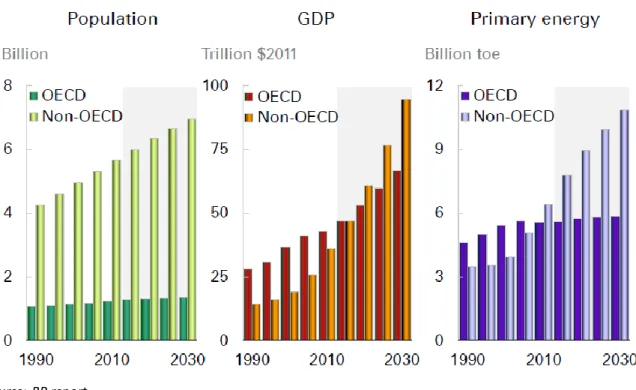
According to the BP Energy Outlook 2030 (BP report), the worldwide demand for energy will be growing for the next 15 years, driven by the increasing income level, around double in 2030, and the world population evolution, almost more 1.3 Billion people consuming energy.
Figure 1: World Energy Drivers
Source: BP report
The world primary energy consumption will be reached 1.6% growth/year, accompanied by the urgent necessity of protecting the environment, reducing the air pollution and CO2 emissions and other pollutants as well. In 1997, the Kyoto Protocol was the first s tep of the
world climate change discussion, considered at that time a milestone regarding the world environment policy. However, the fact of US did not sign the protocol become its overall impact weakened.
The protocol intentions were reducing the greenhouse gas in atmosphere, by targeting maximum lower quantitative values of emissions to the atmosphere to industrialized countries, attributing extra taxation if they do not fulfil this value. On the other hand, the intentions for developing countries were less restrict, once it is understandable that social and economic developing goals entered in conflict with those environment goals.
Recently, the European Union revised upwards the 2020 target to 20%8 of its total energy
getting from renewable resources, including wind, solar, hydro, geothermal and biomass as well, making possible a stronger reduction of greenhouse emissions but also a necessary diversification in the energy sector diminishing the dependence of fossil fuels.
According to the Global Wind Energy Council (GWEC) report, the main aspect nowadays regarding energy constraints is to find the optimal solution to meet the future energy needs with the necessary rearrange of energy mix, being sustainable and economically advantageous. Over the last 10 years, the power sector fuel mix has changed significantly, given the higher contribution of the non-fossil fuels to this performance. Analyzing the BP
report, the renewables including biofuels are “the fastest growing fuels”9 presenting a 7.6%
growth rate per year between 2011 and 2030. Regarding fossil fuels, gas presents higher growth, around 2%/year, followed by coal and oil, 1.2% and 0.8%/year respectively.
Renewable energy has demonstrated a strong and consistently performance path given the already mentioned necessity of finding alternative and efficient sources of energy, as it is stated in BP Report through the analysis of the growth rate and share evolution of renewables in 2011-2030 period. This path was boosted by favorable regulations and incentives schemes adopted by several countries/governments to supporting ambitious renewable energy values compared with their total production. Based on this set of incentives combining the continuous falling of technology’s costs plus the impact of recent
8
European Commission – Directive of the European Parliament and of the Council, COM (2012) 595 Final
9
crude and carbon prices comportment, globally help to framework the presented stronger growth rates of renewables.
According to KPMG Taxes and incentives for renewable energy (KPMG report), it is recognized that renewable energy delivers several benefits for industries, markets and countries, summarizing to the global economic representatives.
First of all, renewables allow more diversity of supply sources of energy given the increasingly demand, and concede capacity to reduce the importations of fossil fuels, increasing the security and diversity of energy. Secondly, renewables has an active role in environment protection and economic growth, contributing to the reductions of CO2 emissions and being an important part of different countries’ recovery economic plans, namely associated with significant job creation and lower energy bills . Finally, responding to a continuously higher demand of electricity and to service part of population without access to electricity, renewables increase the access and affordability of energy.
According to the KPMG report, renewables trends for 2014 have been suggesting a year of industry’s maturation based on changing investors options, lower values of global investments, the government policies, the role of emerging markets and the develop of other subsectors of renewables.
Also the BP Report underlying this idea, considering that renewables face a future set of challenges, leading by the key growth limitary factor, the affordability of subsidies. Diminishing investment costs allow maintaining the subsidy burden at a sufficient level to incentive the renewables scale up. Nevertheless, it is stated that renewables are expected to maintain a growing path, supported essentially by emerging markets once they are able to sustain higher growth rates and significant profitable opportunities. Parallel, the subsidies issue is gaining relevance in the market and in the industry analyses, due the fact it is an important part of the return equation and investment projects decisions, justification for shifting business focus of major renewables companies. EDPR is one of these companies stating that its expansion plan will focus mainly on emerging markets, Brazil and now Mexico, and US and Canada.
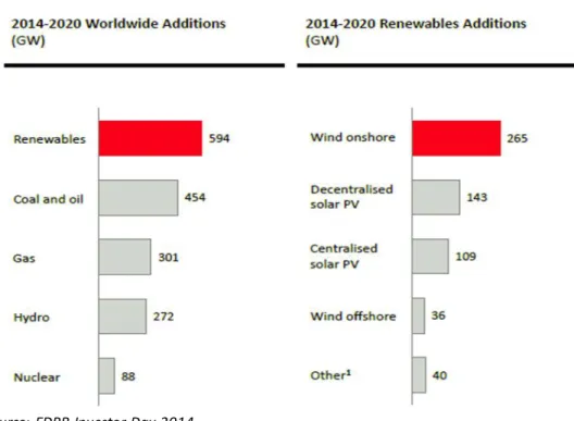
According to the data presented by EDPR, renewables will represent the higher amount of additions regarding different type of energy sources, almost 594 GW between 2014 and 2020. More, inside renewables segment, the wind onshore is largely the source of energy with more additions achieving nearby 265GW, followed by solar PV – decentralized and centralized- and wind offshore.
Figure 2: Worldwide and Renewable Additions
Source: EDPR Investor Day 2014
The core competencies of EDPR are focused on wind energy as we already explained above, reason why we will explore now in more detail the wind energy industry, its performance drivers and evolution, discussing the main trends and possible future options of this industry in several different markets.
2.2. Wind Energy Industry
2.2.1. World portfolio – Re-shifting of installed capacity
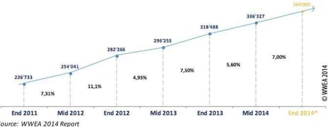
According to the World Wind Energy Association (WWEA) – 2014 half-year report (WWEA report), since 2011 the wind world capacity registered a successively increase, underlying that the total installed wind capacity expected for end 2014 will achieve 360.000 MW, representing an annual increase of 7%.
Figure 3: World Wind Capacity 2011-2014 (MW)
Source: WWEA 2014 Report
Summarizing all reasons appointed to the development of renewables, the wind energy development bases essentially on the economic advantages, the increasing competitiveness relative to others energy’s sources and pressing necessity to mitigate air contamination and climate changes with emission free technologies.
The wind market of energy is dominated by the five wind traditional countries: China, Germany, US, Spain and India. These countries represent almost 72% of the total world wind
capacity, being responsible for 62% of the total capacity additions in first semester of 201410.
The dynamism of the market is extended to all continents, with new installations in South Africa and other Africans countries, but also an increasing of capacity in Brazil , Sweden, Poland and Australia.
Firstly, the Asiatic market accounts 36.9% of total installed capacity in the world, crossing the share of Europe of 36.7%, confirming the boost that Asiatic countries are experiencing. China and India are the responsible for that achievement since they present optimistic prospects given new ambitious plans for wind energy developments. The contributions of this market are only constrained by the nuclear lobby that yet exists in some countries, as Japan or Korea, avoiding the clear industrial and economic advantages.
Secondly, the European market is largely leaded by Germany, with a total capacity around 35.5GW. Spain, UK, France and Italy complete the Europe top five based on installed
10
capacity. However, the additions of new capacity are showing relative stabilization in some countries, as Spain and Italy, and a continuous increasing in others, as France, Sweden and UK. This situation is justified by the expected revision of 2030 European renewables energy targets and the clarification of the Ukraine situation.
Thirdly, the North American market faced a dramatic decline during the first part of 2013 year, regarding the uncertainty over the extension of Production Tax Credit (PTC) and Investment Tax Credit (ITC). PTC and ITC are similar fiscal incentives to renewable producers, remunerating the production and the investment, respectively, being updated every 2-3
years, as the MACRs incentive as well11.
After the approval of the incentives extension, the market has started its recovery based on a higher competitiveness and increasing support schemes, even the signals sent by the federal level were not positive as expected. Canada is assisting a growing phase, installing more 92% in this first semester compared with the first semester of previous year, helping the overall development of the whole region market, but more important, becoming “the
sixth largest market of new wind turbines worldwide”12.
Fourthly, the Latin American market is essentially dominated by Brazil. Brazilian market
represents the 13th largest user of wind energy, accounting a total capacity of 4.7GW given
an impressive growth rate of 38.2% in this 1st semester. It is expectable that Brazil achieves
the top ten countries with more installed capacity in the end of 2014, being possible that other Latin American countries emerge with modest growth levels.
Finally, the offshore market starts appearing as the next global movement for the wind industry. The Roland Berger Work states that offshore will be crucial for European countries in order to achieve the climate and energy targets pre-defined to 2020, namely the 40GW installed offshore capacity. It also argues that offshore has several advantages that justify this growing strategy. Firstly, the maturity of the wind industry; secondly, offshore seems to be the best solution for countries with higher population density; and finally, it presents higher availability than wind onshore, and larger room for improvements regarding costs reductions. 11 Appendix 13 12 WWEA Report
2.2.2. “Are renewables energies a luxury?” – Cost competitiveness
Renewables energies – wind onshore specifically – create a unique opportunity to policymakers develop a solution for the related problems with conventional technologies. Wind is nowadays a cost competitive source, as we will explain further, with a general high level of availability, even at different speeds levels based on different geographical locations. It is important to underling that wind is a zero marginal cost technolog y, representing a comparative advantage vis-à-vis coal, nuclear energy or natural gas once it is cheaper, in first plan, and in second plan, it creates a protection from fuel prices and government decisions uncertainty.
The decision in which technology to invest in, conventional or renewables, it is one of the most debated questions in utilities industry and it has dividing the market. The literature states that for this specific analysis, it should be used the Levelised Cost of Energy (LCOE), “(…) the primary metric for describing and comparing the underlying economics of power
projects”13. LCOE combines all expected lifetime costs, since construction, operational and
financial, required to guarantee wind farms fully operation, and the expected revenues and production streams. Both cost and revenues are adjusted to the inflation and the set is discounted to obtain the present value.
Figure 4: LCOE of Wind industry derivation
Source: IRENA report
13
IRENA, “Renewable Energy Technologies: Cost Analysis Series – Wind Power”, Volume 1: Power Sector, Issue 5/5, June 2012
As we can analyze from the graph above, in terms of LCOE, wind onshore competes with all technologies, getting a LCOE of €68/MWh. The LCOE of wind onshore is lower than some conventional energy technologies, as coal or nuclear, due the fact of a decreasing investment cost per MWh, based on scale economies and technology progress, and also overall increasing its competitiveness.
More, EDPR indicates that onshore wind projects with high load factors are already
competitive with new combined cycle gas turbine (CCGT) power station14, a truly
competitive alternative energy source, even there are renewables technologies that must develop their mature state and continue to increase their competitiveness to be a reasonable future solution.
The load factor is an important element when we are analyzing the performance of a wind farm, being influenced by the turbines characteristics, wind resources and consequently achieved total production. It is usually accepted an average value between 25% and 30%, even it can change widely considering different geographical regions, different wind resources, or even different turbines as it stated by the Partnerships for Renewables and confirmed further in our valuation, in EDPR operational case.
According to the IRENA (2012), the wind industry faces a relative simple structure of costs when is starting a new project: Capital Costs and Operating Costs.
On one hand, the capital costs, or usually denominated Capex, aggregate the expenses of wind turbines, foundation, grid connection, planning & miscellaneous, among others. On the other hand, operating costs aggregates the Levies and Opex, being the latter usually segmented in O&M, Personnel costs and SG&A.
14
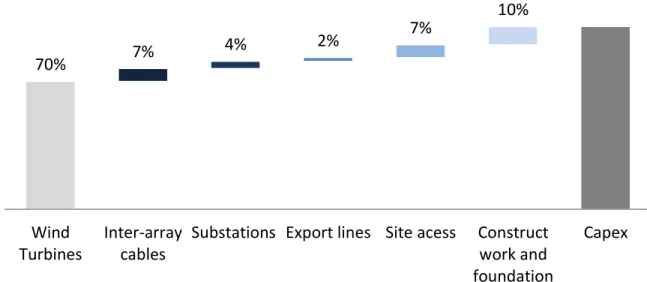
Figure 5: Capex Wind Onshore breakdown
Source: E.ON Wind Factbook
It is noticeable the parallel path existing between wind energy industry and the wind turbines industry. Bearing in mind a construction of an onshore wind farm, the wind turbines represents around 70% of capex during the construction phase and during the lifetime of the project represent a fixed maintenance part of O&M total costs, accordingly to E .ON Wind
Factbook15. The importance of strong agreements and competition among turbines suppliers
is so justified, being the base of future substantial reductions regarding the required initial investment on wind farms.
2.2.3. Regulatory systems
One of the main discussed assumptions regarding renewables is that the late are expensive compared with other technologies, given an analysis between renewables costs and electricity wholesale market prices. Renewable technology has marginal variable costs and currently a set of priorities regarding the market, as preferred injection of production in the market.
The wholesale market pressures the companies’ variable costs and creates competition among entities, benefiting from the pressure to lowering the wholesale price, tending to
zero when there is a strong renewable production16.
15
See Appendix 11
16
EDPR’s example in Spain, where with high wind generation (December 25th 2013), the wholesale price achieves €5/MWh 70% 7% 4% 2% 7% 10% Wind Turbines Inter-array cables
Substations Export lines Site acess Construct
work and foundation