1
Is the Euro-Area Core Price Index Really More
Persistent than the Food and Energy Price Indexes?
José Manuel Belbute
Department of Economics, University of Évora, Portugal
Center for Advanced Studies in Management and Economics - CEFAGE, Portugal jbelbute@uevora.pt
Abstract
The purpose of this paper is to measure the degree of persistence of the overall, core, food and energy Harmonized Indexes of Consumer Prices for the European Monetary Zone (HICP-EAs) and to identify its implications for decision-making in the private sector and in public policy.
Using a non-parametric approach, our results demonstrate the presence of a statistically significant level of persistence in four HICP-EAs: headline, core, food and energy. Moreover, contrary to popular belief, the core index does not reflect permanent price changes. We also find evidence that the food and energy price indexes are more volatile and more persistent than the other two price indexes. Our results also show a reduction in persistence for both the headline and the core price indexes after the implementation of the single monetary policy, but not for food and energy.
These results have important implications for both the private sector and for policymakers who use the core as a reference price index for their decision-making because the use of this index can lead to an erroneous perception of price movements.
Keywords: Harmonized Index of Consumption Prices, Core Inflation, Euro Area, Persistence JEL Classification: C14, C22, E31, E52
Paper prepared for the 32º Meeting of the Brazilian Econometric Society Salvador, December 2010
2
Is the Euro-Area Core Price Index Really More
Persistent than the Food and Energy Price Indexes?
1. Introduction and Motivation
Inflation persistence has been a central issue in macroeconomics for the last decade due to its implications for the design, implementation and effectiveness of monetary policy. In the specific case of the European Monetary Union (or European Area, hereafter E.A.), the implementation of a single monetary policy was responsible for a decline in inflation persistence after 1999, signaling that the European Central Bank (hereafter ECB) has been able to ensure that actual inflation does not deviate for too long and too persistently from the level announced by the bank and from its medium-term inflation target.
Most of the literature on the subject focuses on topics like the degree of persistence in inflation or whether inflation has changed as a result of a shift in the strategy of monetary policy towards “inflation targeting.” The papers of Levin and Piger (2003), Willis (2003), Gadzinsky and Orlandi (2004), Cogley and Sargent (2008), Altissimo et al. (2006), Corvoisier and Mojon (2005), Piveta and Reis (2007), Marques (2004) and Dias & Marques (2010) are a few examples of the many important contributions to the literature on inflation persistence All of these papers compute persistence by estimating the sum of the autoregressive coefficients1 using inflation data extracted from the aggregate private consumption, gross domestic product deflators, the consumer price index (for the USA) or the harmonized index of consumer prices (headline or overall, core, food and energy for the E.A.) time series.
Core inflation is one of the leading indicators upon which both individual and institutional economic agents base their decisions and anchor their expectations. Households, governments, unions, central bankers, etc. tend to perceive core inflation as an indicator of long-lasting change in prices. In contrast, overall inflation is seen as an indicator of a mix of both permanent (long-lasting) and transitory changes in prices that may cause erroneous perceptions of price trends, thereby leading to erroneous decisions.
Core inflation is obtained by extracting the two most volatile components from the overall price index (that is, food and energy prices), arguably to obtain a smoother and less volatile time series that supposedly better reflects long-term (or permanent) price movements.
1
Marques (2004), and Dias & Marques (2010) also use a non-parametric method to measure inflation persistence.
3
Because they are more volatile, the food and energy price indexes reproduce transitory price movements and are, therefore, perceived as being less persistent.
The purpose of this paper is to measure the degree of persistence of the overall, core, food and energy Harmonized Indexes of Consumer Prices for the European Monetary Zone, neither seasonally nor working-day adjusted (hereafter HICP-EAs) and to identify its implications for both the design of monetary policy and the management of inflation expectations in the Euro Area. In particular, we test whether the core price index of the E.A. reflects long-lasting instead of temporary price level movements, as is commonly believed. We measure the degree of persistence using a non-parametric methodology proposed by Marques (2004) and Dias & Marques (2010). This new measure of persistence is based upon the relationship between persistence and the concept of mean reversion and can be defined as the unconditional probability of a (either a stationary or a non-stationary) stochastic process not crossing its mean in time t.
Our results show that we cannot reject the presence of a process of persistence in all-time series even though not all are equal. In particular, the persistence of the overall HICP-EA does not significantly differ from the core HICP-EA and both of these indexes are statistically less persistent then the food and energy price indexes. We also find that, contrary to common belief, the most volatile HCP Indexes (food and energy) are also the most persistent. Moreover, extracting the most volatile components of the overall HICP does not generate a time series that better reflects the permanent price-level. Our findings also confirm that after the implementation of the single monetary policy in the E.A., there was a decline in persistence for both the aggregate and the core price indexes, while the food and energy indexes did not change their level of inertia after the creation of the Euro. This finding suggests that the European Central Bank (hereafter ECB) was able to anchor inflation expectations to its policy goal, regardless of the long-lasting increases in food and energy prices.Moreover, these results have important implications for both the private sector and for policymakers who use the core as a reference price index for decision-making because the use of this index can lead to an erroneous perception of price movements.
The rest of the paper is organized as follows: Section 2 offers some methodological notes about persistence. Sections 3 and 4 present the data and our results. Section 5 concludes the paper.
4
2. Persistence: definitions and methodological notes
This section briefly presents the concept of persistence, discusses the manner in which it is measured when the time series is not stationary and presents some methodological notes regarding the test of a change in the level of persistence between two periods.
Persistence is a well-known concept from the macroeconomic literature. The papers of Rotemberg and Woodford (1997), Huang and Liu (2002), Ascari (2003) and Wang and Wen (2006) are examples of contributions to the literature that focus on staggered price and staggered wage-setting as causes of persistence in the major macroeconomic aggregates. Moreover, the articles of Frankel and Rose (1996), Cheung and Lai (2000) and Murray and Papell (2002) are examples of measurements of the persistence of PPP deviations from equilibrium, while the papers of Guender (2006), Giugale and Korobow (2000), are examples of contributions to the literature that relate persistence of output and of inflation with the degree of openness of the economy and the exchange-rate regime. Maury and Tripier (2003) and Bouakez and Kano (2006) suggest that persistence mechanisms are inherent to the propagation of the causal effects of temporary shocks, such as policy measures, and, therefore, capable of explaining the (strong) persistence of output. Finally, Belbute and Caleiro (2009) find evidence of a strong process of persistence in aggregate and disaggregate private consumption.
There are several definitions of persistence in the literature and they all share the concept that persistence is related to the speed of a variable’s response to a shock (see, for example, Marques (2004)). In this paper, we adopt the definition proposed by Marques (2004) and Dias & Marques (2010) and define persistence as the speed with which a variable converges to its equilibrium after a shock. A variable is said to be the more (less) inertial the slower (faster) it converges (or returns) to its equilibrium after the occurrence of a stimulus. In other words, when the value is small, a variable responds quickly to a shock, tends to deviate from its trend briefly and therefore its changes tend to be temporary. Conversely, when the value is high, the speed of adjustment is low and the shock tends to have long-lasting effects.
The usual way to capture a variable degree of persistence is by the estimation of the sum of the autoregressive coefficient given by the well-known univariate AR(k), whose reparameterization may be given by the following expression:
5
(1)
where denotes the variable at moment t,
is the “sum of the auto-regressive coefficients”, , and
(2)
is the “unconditional mean” of series.
This formulation has the advantage of demonstrating that persistence is related to the concept of “mean reversion,” represented in equation (1) by the term As long as 2
any unit deviation from the mean in period t-1, , will force the series to a (positive or negative) change in the following period by the amount , thus bringing it close to the mean.3 Therefore, Andrews & Chen (1994) proposed the “sum of the autoregressive coefficients” as a measure of persistence.4 The rationale for this measure comes from the fact that for , the cumulative effect of a shock on is given by . One important implication of the stationary autoregressive processes case (that is, ) is that any random shock has transitory effects on the variable, while under the autoregressive unit roots hypothesis case (that is ), its effects on the system are long-lasting. Moreover, although the temporary effects of a shock may vary in length, under the unit roots hypothesis, the system will never return to its trend after a shock.
Unfortunately, the existence of a unit root in the data generation process makes it impossible to accept the results from a traditional OLS estimation and the procedure described above is infeasible. Marques (2004) and Dias & Marques (2010) have suggested a non-parametric measure of persistence, , based on the relationship between persistence and mean reversion. In particular, they suggested using the statistic:
(3)
2
In his case, the time series is said to be stationary or, equivalently, it does not have an autoregressive unit root.
3
By definition, a unit root process does not exhibit this property of mean reversion.
4
Authors have indeed proposed other alternative measures of persistence such as the largest autoregressive root, the spectrum at zero frequency, or the so-called half-life. For a technical appraisal of these other measures see, for instance, Marques (2004) and Dias & Marques (2010).
6
where n stands for the number of times the series crosses the mean during a time interval with T + 1 observations. The ratio n/T gives the degree of mean reversion and can be seen as the unconditional probability of a given series not crossing its mean in period t.
This alternative measure of persistence, , has the advantage of not requiring any particular specification for the data generation process, but rather extracts the determinist component of the series using an appropriate approach.5 Moreover, this method is also robust to the presence of outliers in the data. Naturally, the model is sensitive to the method used to de-trend the data series, but it is particularly well suited to the empirical evidence of changing means.
By definition, this measure varies between 0 and 1. In the context of a symmetric white noise process with mean zero, when we have evidence of the absence of significant persistence. When we find evidence of greater persistence and with values below 0.5 we find evidence of negative autocorrelation.
The nonparametric degree of persistence of the four HICP-EAs will be evaluated assuming the presence of a long-term changing mean and using the cyclical component of each series extracted by the Hodrick-Prescott filter (1981).
Finally, we look at persistence conditional to an unknown break in the mean for each time series and for the whole sample using the strategy proposed by Dias and Marques (2010) by estimating the following model:
(4)
where equals 1 if the time series crosses its mean and zero otherwise and is a dummy variable that is 0 and 1 otherwise. From (5), we can write that and where and are, respectively, the persistence measures for the first and second sub-period. Therefore, testing the change of persistence amounts to a test of whether is significantly different from zero.
3. Data and preliminary data analysis
This section describes the basic dataset, presents the results of the unit root tests and discusses the implications for persistence of the non-stationary nature of the data.
3.1 A brief description of the dataset
7
We use the monthly E.A. HICP data (Harmonized Index of Consumer prices (HICP-EA hereafter)) from January of 1995 through January of 2010 from Eurostat to measure the degree of persistence for four series (neither seasonally nor working-days adjusted): 1) HICP all items, 2) all items excluding food and energy HICP (also known as “core”), 3) food HICP and 4) energy HICP.
The HICPs are economic indicators constructed to measure changes over time in the prices of consumer goods and services acquired by households. The HICPs give comparable measures of inflation in the euro zone.6 They are calculated according to a harmonized approach and a single set of definitions. They provide the official measure of consumer price inflation in the euro zone for a wide variety of purposes, including: as a guide for monetary policy; for assessing inflation convergence as required under the Maastricht criteria; for the indexation of commercial contracts, wages, social protection benefits or financial instruments; as a tool for deflating the national accounts or calculating changes in national consumption or living standards, etc.7
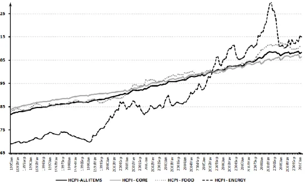
Conceptually, the HICPs are ‘Laspeyres-type price indices8’ or ‘pure price’ indexes that measure the average price change on the basis of the changed expenditures required to maintain household consumption patterns and the composition of the consumer population in the base or reference period. Strictly speaking, ‘pure’ means that only the changes in prices are reflected in the measure between the current and the base or reference period. The HICPs are not a cost-of-living index. That is, they are not a measure of the change in the minimum cost for achieving the same ‘standard of living’ (i.e., constant utility) from two different consumption patterns in two compared periods and where factors other than pure price changes may enter the indexes. The key role of the HICPs is, therefore, to measure price stability. Figure 1 plots the four time series used in the study.
6
As well as for the EU, the European Economic Area and for other countries including accession and candidate countries
7
HICP data, including backdata, is revisable under the terms set in Commission Regulation (EC) Nº 1921/2001. When updated, the database overwrites existing data with the revised data and those changes will only be flagged for a short period, generally until the next update.
8
The indices are based on the prices of goods and services available for purchase in the economic territory of the Member State for the purpose of directly satisfying consumer needs. It should be noted that the decision to adopt this specific method was supported by the most widespread definition of inflation: “… a persistent increase in the general level of prices.”
8
Figure 1 – Harmonized Consumer Price Indexes
For the whole-period sample, the average core inflation rate (both monthly and annual) was lower than the other three inflation measures. However, Table 1 also shows that although many products included in the index of core inflation, such as transportation or plastic-made goods, are directly influenced by energy prices, the core inflation rate was almost half the energy inflation rate. This suggests that firms’ final prices did not reflect the higher energy cost that they eventually had to face.
Regarding the level of volatility of the four HICP-EAs, we find that, as expected, energy and food are the most volatile price indexes. However, when they are excluded from the overall price index, the resulting time series, the HICP core, becomes more volatile than the original series.
Table 1. Inflation rate and HICP volatility
HCPI-ALL ITEMS HCPI - CORE HCPI - FOOD HCPI - ENERGY
Average monthly rate of inflation 0,16% 0,13% 0,16% 0,28%
Standard deviation (pp) 0,271 0,350 0,428 1,415
Average annual rate of inflation (chain) 1,89% 1,61% 1,98% 3,40%
Standard deviation (pp) 0,760 0,412 1,870 6,119
9
3.2 Testing stationary
We test the unit roots hypothesis for the four HICPs using the modified Dickey–Fuller t test proposed by Elliott et al. (1996) and also the KPSS test for the null hypothesis of stationarity (Kwiatkowski et al., 1992). The AD-GLS t-test strongly suggests that the null hypothesis of a unit root cannot be rejected for all variables at the 5% significance level.9 Moreover, the KPSS stationarity test rejects the presence of a stationary linear trend for all four price index series. As expected, stationarity could not be rejected for inflation for the four time series.
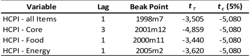
One major problem with the unit roots test is the implicit assumption that the deterministic trend is well determined. However, as Perron (1989) argued, if there is a break in the deterministic component of the time series, then unit root tests will lead to misleading conclusions about the (non)stationarity tests. The literature on trend breaks in unit roots is vast and sometimes controversial, but converges upon the need to test the null hypothesis of a unit root with a possible known and/or unknown broken point. In our empirical analysis, we fully considered the possibility of unknown structural breaks in both the drift and the trend for the four HICPs. To test for a break in the mean, we choose the Zivot and Andrews (1992) test that allows testing for an unknown break in the mean. We imposed 20% symmetric trimming to avoid detecting spurious breaks at the beginning and/or at the end of the sample. We were able to find four statistically significant mean breaks for which the unit root hypothesis could not be rejected (see Table 2). The optimal time lag was chosen using BIC.
Table 2. Unit roots tests allowing for one unknown break point
Variable Lag Beak Point tt tc (5%)
HCPI - all Items 1 1998m7 -3,505 -5,080
HCPI - Core 3 2001m12 -4,859 -5,080
HCPI - Food 1 2000m11 -3,440 -5,080
HCPI - Energy 1 2005m2 -3,620 -5,080
These breaks are consistent with the emergence of the euro and with the implementation of a single monetary policy in 1999. We use these breaks to measure persistence conditional to a break in the mean for each HCP index.
9
The tests were also done using log-levels, and we consistently found that we cannot reject the null hypothesis of nonstationarity at the 5% level of significance.
10
4. The level of persistence of the overall, core, food and energy HCP indexes.
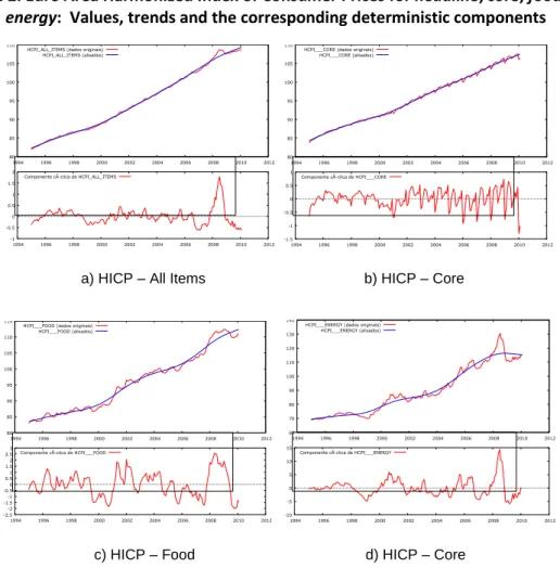
This section measures the level of persistence of the four HICP-EAs. A simple visual inspection of the graphs of all-time series samples suggests that the measurement of the level of persistence should be performed under a time varying mean framework. Moreover, given the strong evidence of nonstationarity of all times series, the use of the non-parametric method proposed by Marques (2004) and Dias & Marques (2010) to measure persistence is appropriate. We do that by extracting the cyclical component using the H-P filter. The H-P filter is a well-known method to obtain the smoothed non-linear representation of a time series. Formally, the trend component (or mean) t of the time series is the solution of the following
minimization problem: (5)
i.e., the H-P filter seeks to minimize (penalizes) the cyclical component subject to a smoothness condition reflected in the second term. The second term penalizes variations in the growth rate of the trend component. The larger the value of λ, the higher the penalty and thus, the smoother the trend will be. In the limit, as goes to infinity, the filter will choose for approximating a linear trend. Conversely, for , we get the original series.
The H-P filter is a very flexible device because it allows us to approximate many commonly used filters by choosing appropriate values of . Hodrick and Prescott have suggested using values for of around 1600 for quarterly frequency data. A simple and common way to get the value of is to multiply the square of the data frequency by 100. Given that our data is of monthly frequency = 14.400, the cyclical components of our data series are plotted in the graphs below.
11
Figure 2. Euro Area Harmonized Index of Consumer Prices for headline, core, food and
energy: Values, trends and the corresponding deterministic components
a) HICP – All Items b) HICP – Core
c) HICP – Food d) HICP – Core
The non-parametric methodology confirms the presence of a significant high degree of persistence for all four HICP indexes (see Table 3). Moreover, the null hypothesis of absence of persistence for the four indexes of persistence can be rejected at a test of 1% significance level.
Table 3. Level of persistence of HCP indexes for E.A. (1995-2010)
Variable
HCPI - All items 0,7473 0,0323 *** HCPI - Core 0,7692 0,0313 *** HCPI - Food 0,8791 0,0242 *** HCPI - Energy 0,8571 0,0260 ***
se
Note:
*** Denotes the rejection of the null of (absence of persistence) at a 1% significance level 80 85 90 95 100 105 110 1994 1996 1998 2000 2002 2004 2006 2008 2010 2012 HCPI_ALL_ITEMS (dados originais)
HCPI_ALL_ITEMS (alisados) -1 -0.5 0 0.5 1 1.5 2 1994 1996 1998 2000 2002 2004 2006 2008 2010 2012 Componente cÃclica de HCPI_ALL_ITEMS
80 85 90 95 100 105 110 1994 1996 1998 2000 2002 2004 2006 2008 2010 2012 HCPI___CORE (dados originais)
HCPI___CORE (alisados) -1.5 -1 -0.5 0 0.5 1 1994 1996 1998 2000 2002 2004 2006 2008 2010 2012 Componente cÃclica de HCPI___CORE
80 85 90 95 100 105 110 115 1994 1996 1998 2000 2002 2004 2006 2008 2010 2012 HCPI___FOOD (dados originais)
HCPI___FOOD (alisados) -2.5-2 -1.5-1 -0.5 0 0.5 1 1.5 2 2.5 3 1994 1996 1998 2000 2002 2004 2006 2008 2010 2012 Componente cÃclica de HCPI___FOOD
60 70 80 90 100 110 120 130 140 1994 1996 1998 2000 2002 2004 2006 2008 2010 2012 HCPI___ENERGY (dados originais)
HCPI___ENERGY (alisados) -10 -5 0 5 10 15 1994 1996 1998 2000 2002 2004 2006 2008 2010 2012 Componente cÃclica de HCPI___ENERGY
12
Nonetheless, we could not reject the null of equal persistence between HICP-all items and HICP-core, as well as HICP-food and HICP-energy. However, our results also provide statistically significant evidence for differences in persistence among the four indexes at a 5% significance level. In particular the HICP-food and HICP-energy indexes are more persistent than the overall and the core HICPs. Moreover, these two price indexes are also the two most volatile HICP components (see Table 1). Given that food and energy price movements tend to be long lasting, the previous results contradict the current thinking about the relationship between volatility and persistence. Therefore, a volatile time series is not necessarily less persistent and vice versa.
Additionally, given our definition of persistence, food and energy prices tend to move away from and/or return to their trends more slowly than the overall and core HICPs. Moreover, changes in food and energy prices tend to be more long-lasting than changes affecting the core index. Therefore, a random shock affecting the core (and the overall) HICP will cause temporary effects, whereas the same shock will have more permanent effects on the food and energy price indexes.
Core HICP is built under the assumption that the most volatile and temporary price movements are removed from the overall index. Despite this assumption, the resulting time series is not more persistent. The fact that the core price index is both less persistent and less volatile has the important implication that price movements remain essentially temporary in the new series. Therefore, both private and public agents using the core HICP may hold erroneous perceptions of permanent price movements.
Finally, we tested the null hypothesis of change in persistence in the dates identified by Zivot and Andrews’ (1992) unit roots tests (see Table 2) and we consistently find that before the breaks, all four HICPs exhibit a high degree of persistence. Additionally, our results also suggest that the level of persistence does not differ significantly among the four HICPs.
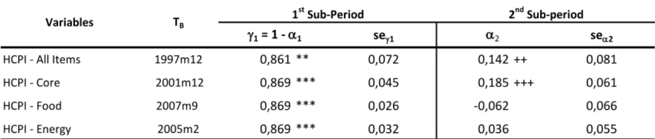
Table 4 – Testing changes in persistence between the two sub-periods
se1 sea2
HCPI - All Items 1997m12 0,861 ** 0,072 0,142 ++ 0,081
HCPI - Core 2001m12 0,869 *** 0,045 0,185 +++ 0,061 HCPI - Food 2007m9 0,869 *** 0,026 -0,062 0,066 HCPI - Energy 2005m2 0,869 *** 0,032 0,036 0,055 TB Variables 1 st Sub-Period 2nd Sub-period 1 = 1 - a1 a2 Notes:
13
** Denotes the rejection of the null of absence of persistence at a 5% significance level +++ Denotes the rejection of the null of no change of persistence at a 1% significance level ++ Denotes the rejection of the null of no change of persistence at a 5% significance level
However, after the breaks, we find that the estimated persistence is lower for both the aggregate (0.719) and the core (0.684) HICPs, whereas we could find no significant evidence that persistence changed over time for the food and energy prices indexes.
5. Conclusions
Households, firms, governments, unions, central bankers, etc. perceive core inflation as an indicator of long-lasting change in prices and use it to form their expectations for current and future inflation. Core inflation is obtained by extracting the two most volatile components of the overall price index (food and energy prices), so the resulting index is thought to describe the more stable inflation rate of non-food and non-energy items. Moreover, given that volatility is often associated with temporary movements, ignoring changes in food and energy prices also suggests that changes in prices of these two items are temporary.
Our paper investigates these issues using a new non-parametric measure of persistence proposed by Marques (2004) and Dias and Marques (2010). Persistence is broadly understood as the unconditional probability of not crossing the mean in time t.
Our results show the presence of a statistically significant level of persistence in the four E.A. harmonized consumer price indexes: overall (or headline), core, food and energy. The degree of persistence of the core price index is not significantly different from that of the overall price index. This suggests that extracting the most volatile components of the general price index does not generate a new series (the core) that is less volatile and more persistent than the original. In other words, for the whole sample period, the E.A. core consumer price index did not describe a less volatile behavior than the original index.
The degree of persistence also does not differ statistically between the food and energy price indexes. Moreover, they are both statistically higher than the other two price indexes. That is, for the whole sample period, we find that changes in food and energy prices were more permanent than in the headline and core price indexes. In particular, we find evidence suggesting that the core price index does not measure permanent price movements and, therefore, permanent inflation. This is an unexpected result, given that food and energy prices have been rising steadily since 2003 and that many products included in the index of core inflation, such as transportation or plastic-made goods, may be directly influenced when the real price of energy changes permanently. Given that the ECB was able to successfully anchor
14
inflation expectations to its target, a possible explanation for this result is that firms may perceive energy price movements as temporary and accordingly tend to reduce profit margins rather than increase final prices.
We also find that, contrary to common belief, a more volatile variable is not necessarily a less persistent one. In other words, the food and energy price indexes are more volatile than the headline and core price indexes, but they nevertheless reflect long-lasting price changes. Finally, our findings suggest that after the breaks, there was significant evidence of a strong reduction of persistence for both the aggregate and the core, whereas the food and energy indexes did not change their level of persistence.
These results have important implications for both the private sector and for policymakers who use the core as a reference price index for decision-making because the use of this index can lead to an erroneous perception of price movements. Contrary to common belief, the core price index is not a measure of permanent price changes; therefore, using it as a reference of long-lasting price changes may lead to biased policy decisions.
15 References:
Altissimo, F., M. Ehrmann, F. Smets (2006); Inflation Persistence and Price Setting in the E.A.: A Summary of the IPN Evidence, Occasional Paper nº 46, European Central Bank.
Ascari, G., (2003), “Price/Wage Staggering and Persistence: A Unifying Framework”, Journal of Economic Surveys, 17, 511-540.
Belbute, J. and A. Caleiro (2009), “Measuring the Persistence on Consumption in Portugal,” Journal of Applied Economic Sciences, IV, 2(8) (Summer), 185-202.
Bouakez, H., Kano, T., (2006), Learning-by-doing or habit formation?, Review of Economic Dynamics, 9, 508-524.
Cheung, Y. and K. Lai (2000), On the Purchasing Power Parity Puzzle, Jornal of INtenational Economics, 52, 321-330.
Cogley, T., Primiceri, G.E., Sargent, T.J., (2008), Inflation-Gap Persistence in the U.S.Working Paper No. 13749. National Bereau of Economic Research.
Corvoisier, S. and B. Mojon (2005); Breaks in the Mean of Inflation: How They happen and What to do With Them. Working Paper nº 451, European Central Bank.
Dias, D. and C. Marques (2010); Using Mean Reversion as a Measure of Persistence, Economic Modeling, 27, 226-273.
Elliot, G., T. Rothemberg and J. Stock (1996), Efficient Tests for an Autoregressive Root, Econometrica, 64, 813-836.
European Comission, (2004); Harmonized Indices of Consumer Prices (HICP), European Comission, Eurostat. Luxembourg.
European Comission, (2001); Compendium of HICP Reference Documents, European Comission, Eurostat. Luxembourg.
Frankel, J. and A. Rose (1996), A Panel Project on Purchasing Power Parity: Mean Reversion Within and Between Countries, Journal of International Economics, 40, 209-224.
Gadzinski, G., Orlandi, F., 2004. Inflation Persistence in the European Union, the E.A. and the United States. Working Paper 414. European Central Bank.
Giugale, M., Korobow, A., (2000), “Shock Persistence and the Choice of Foreign Exchange Regime: An Empirical Note from Mexico”, World Bank Policy Research Working Paper No. 2371. Available at SSRN: http://ssrn.com/abstract=630755.
Guender, A., (2006), “Stabilising Properties of Discretionary Monetary Policies in a Small Open Economy”, The Economic Journal, 116, 309-326.
Hodrick, R. and Prescott, E.(1981): “Post-war U.S. Business Cycles: An Empirical Investigation,” Working Paper, Carnegie-Mellon, University. Reprinted in Journal of Money, Credit and Banking, Vol. 29, No. 1, February 1997.
Huang, K., Liu, Z., (2002), “Staggered Price-Setting, Staggered Wage-Setting and Business Cycle Persistence”, Journal of Monetary Economics, 49, 405-433.
Kwiatkowski, D., P. Phillips, P. Schmidt and Y. Shin (1992), Testing the Null Hypothesis of Stationary Agsins the Alternative of a Unit Root, Journal of Econometrics, 54, 159-178. Levin, A.T. and J.M. Piger (2003),Is Inflation Persistence Intrinsic in Industrial Economies?
16
Marques, C. R. (2004), “Inflation Persistence: Facts or Artefacts?”, Working Paper 8, European Cemntrall Bank, June.
Maury, T.-P., Tripier, F., (2003), Output persistence in human capital-based growth models, Economics Bulletin, 5, 1-8.
Murray, C. and D. Papell (2002), The Purchasing Power Parity Persistence Paradigm, Journal of International Economics, 56, 1-19.
Perron, P. (1989):The Great Crash, the Oil Price Shock and the Unit Root Hypothesis, Econometrica, 57, 1361-1401.
Pivetta, F., Reis, R., (2007). The persistence of inflation in the United States. Journal of Economic Dynamics and Control 31, 1326–1358.
Rotemberg, J., Woodford, M., (1997), “An Optimization Based Econometric Framework for the Evaluation of Monetary Policy”, In: Rotemberg, J., Bernanke, B., (Eds.). NBER Macroeconomics Annual 1997. Cambridge (MA): The MIT Press, 297-346.
Wang, P.-f., Wen, Y., (2006), “Another Look at Sticky Prices and Output Persistence”, Journal of Economic Dynamics and Control, 30, 2533-2552.
Willis, J.L., 2003. Implications of Structural Changes in the U.S. Economy for Pricing Behavior and Inflation Dynamics. Economic Review, October. Federal Reserve Bank of Kansas City.
Zivot, E. and D. Andrews (1992); Further Evidence on the Great Crash, the Oil-Price Shock and the Unit-Root Hypothesis, Journal of Business & Economic Statistics, Vol. 10, No. 3