The Priips performance scenarios and its misleading shortcomings

(1)

1

A Work Project presented as part of the requirements for the Award of

a Master degree in Finance from the NOVA - School of Business and

Economics

The PRIIPs performance scenarios and its

misleading shortcomings

Maria Teresa Bitetto – 29756

A Project carried out on the Master in Finance Program, under the

supervision of Melissa Prado, professor at NOVA and Saumya Singh,

manager at EY Luxembourg in the Risk and Regulatory Services

department.

(2)

2 From July until December 2018, I worked in EY Luxembourg – Financial Services Advisory.

Particularly, I was an intern in the Risk and Regulatory Services department.

During my internship, I had the chance to work on several projects (i.e. regulatory

requirements, business proposal for an EU tender on financial services supporting solutions

for retail investors, communication with several people across the company, clients facing role…).

The major focus was on the PRIIPs regulation. The main goal of this regulation is the

improvement of the transparency among investment products, through the production of a

document, the Key Information Document (KID), which discloses the risk-reward profile of a

certain product. Indeed, EY Luxembourg helps asset managers to fulfil the increasing

regulatory requirements.

However, during my work experience, I realized, together with my PRIIPs team, that there are

several shortcomings related to this regulation.

Indeed, is the PRIIPs KID really able to give a better overview of the risk?

Through this report, under the supervision of the manager Saumya Singh, and the professor

Melissa Prado, I have shown the biggest failures of a specific requirement of PRIIPs, the

(3)

3

Table of Content

Executive Summary ________________________________________________________ 4

1.Introduction ____________________________________________________________ 6

1.1.The Financial Crisis ______________________________________________ 6 1.2.The new European Regulatory Framework ____________________________ 9

2.The PRIIPs regulation __________________________________________________ 13

2.1.The PRIIPs regulatory technical standards ___________________________ 14 2.2.The PRIIPs Shortcomings – Performance Scenarios ____________________ 15

3. Conclusion ___________________________________________________________ 32 4. References ____________________________________________________________ 33 5. Annex _______________________________________________________________ 36

(4)

4

Executive Summary

The international financial crisis of 2007, was one of the worst crises in recent history, for its magnitude and its impact all over the world.

In Europe, the crush was turned into a sovereign debt crisis. Despite the European Union (EU) and the International Monetary Fund (IMF) adoption of austere measures as financial support condition, the crisis persisted for more than 10 years. As the president of the European Central Bank, Mario Draghi1_{, said, in 2017 the Eurozone was finally out of the crisis. In essence,}

Greece and Spain have finally exited their bailout program, Portugal and its Prime Minister Antonio Costa’s “anti-austerity” government, have cut the deficit to its lowest level in more than 40 years.

However, the recovery has been very slow and still further progresses are needed. The banking sector is fragile, and more reforms should be implemented. It is worthless to say that there are several factors that led to the crisis. Although, many agree that one of the main causes was the lack of a consistent regulation concerning the transparency and accountability requirements in the market. The economic system has worked many years without any Supervisory authority to control it. Indeed, the financial system has always brought innovative instruments within the market. Unfortunately, this innovation was not supported by any new or past regulation, and there were no financial intermediaries for the new instruments. Furthermore, the market, excited for the innovation and the benefits it could offer without any government intervention, did not consider the potential failures.

As a result, a new regulatory framework has been introduced by the European entities, to ensure transparency within the market and the investors. In particular, the PRIIPs regulation, through

1_{See « Tel Aviv, Mario Draghi rassicura: “La crisi nell’Eurozona è finita” », Libero Quotidiano, 17th May 2017, available}

(5)

5 the KID, shall enable a decrease in the level of information asymmetries between the retail investors and the products’ issuers. Despite its goal, the figures related to the KID could be misleading, especially the performance scenarios’ ones. Particularly, as it will be shown further in this work, the performance scenarios base their structure on past data and, consequently, they are not able to capture the unexpected changes in the price trend of a certain product. Furthermore, the missing illustration of past performance is contributing to a not clear visualization of the risk related to a product.

This report has the aim of proving, through the analysis and the tests performed in the Paragraph 2.2., how the PRIIPs performance scenarios cannot be reliable in all the cases, giving in fact a misleading overview on investment solutions.

Indeed, the work wants to highlight that the scenarios could be misguiding and investors have not always the right perception of the risks related to a certain product and could not help in reducing the information asymmetries.

It is important to specify that only PRIIPs Category 2 will be taken into consideration (Paragraph 2.1.), as it is the only Category that EY Luxembourg is advising on.

(6)

6

1. Introduction

1.1. The Financial Crisis

As is well known, the crisis started in the US around 2006, and it is imputable to the sub-prime mortgages. However, its roots date back in 2003, when the number of high-risk mortgages and loans increased significantly. The mortgage subscribers were people that, in different circumstances, would not have obtained the credit requested, since they did not have the necessary guarantees. The factors that have influenced the sub-prime mortgages are related to the US real-estate market and to the securitisation phenomenon. In particular:

- A real-estate bubble was generated by a steady increase in the house prices, from 2000 until 2006. This performance was encouraged by the Federal Reserve (FED) accommodative monetary policy, that kept the interest rates at very low values until 2004, as a consequence to the Internet bubble crisis, and to the attack on the Twin Towers in 2001.

- The above mentioned Monetary Policy allowed the borrowers (i.e. US families) to subscribe mortgages at favourable conditions. The mortgage prices were so convenient that the number of subscriptions rose significantly. This boosted the demand for houses, and, without any increment on the supply side, it led to a mechanism of steady increase of real-estate prices, marking the start of the bubble. Furthermore, the mortgage subscriptions were convenient also for the financial institutions, since, in case of default, they could have recovered the money through the foreclosure and the resell of the houses.

- The Securitisation was developed, a “procedure whereby an issuer designs a financial instrument by merging various financial assets and then markets tiers of the repackaged

(7)

7 instruments to investors. This process can encompass any type of financial asset and

promotes liquidity in the marketplace” (Investopedia definition). Indeed, the credit

institutions could transfer the mortgages to third parties (i.e. special purpose vehicle – SPV, also known as “bankruptcy- remote entity”), once they have been converted into asset-backed securities2_{. As a result, these institutions could receive money before the}

mortgage maturities. The securitisation ensured (at least apparently) banks to get rid of the default risk. This weakened the willing to value properly the customer’s reliability. On the other hand, the SPV financed the acquisition of sub-prime mortgages through the short-term securities offer to investors. Therefore, the procedure of securitisation, together with the lack of an accurate valuation of the assets, allowed the banks to spread highly risk products within the markets.

Considering the low-interest rates, the asset-backed securities were very attractive for both US and European investors, who started to invest in these products. As a consequence, first the risk, and consequently the crisis, could expand also in the Eurozone.

The securitisation contributed to modify the banks’ business model from “originate and hold”, to “originate and distribute”. This means that the banks could have recovered the money lent immediately, through securitisation, and then, they could have used the resources for more mortgages to unreliable borrowers. The financial institutions increased their assets and liabilities in relation to the equity (leverage phenomenon). The related profits were high, but the risk of default was also significant. All these products were sold over the counter (OTC), not in a regulated market. In these circumstances, considering the difficulties of their valuation, the role of the rating agencies has been increasingly important. However, the ratings were subject to model and assumptions, which were not accurate and precise.

2_{See the Investopedia definition: “An asset-backed security is a security that is backed by a pool of loans or receivables. These}

include: auto loans, consumer loans, commercial assets (planes, receivables), credit cards, home equity loans, and manufactured housing loans.”

(8)

8 In 2004, the FED set the interest rates at a higher level, due to the economic revival. The mortgages became more expensive and the number of the defaulted debtors rose. The real-estate demand decreased, and the bubble burst, causing substantial direct and indirect damages. The financial institutions that were more involved, suffered heavy losses. Furthermore, from 2008, the rating agencies downgraded the credit ratings of many asset-backed securities. Most of the securities widely distributed in the markets, became illiquid. Because of the uncertainty, the interbank market experienced a sharp rise in rates. The credit availability was tightened, bringing on a confidence crisis first, and then a liquidity one. The banks suffered because of the SPV and clients default risk exposures, respectively as an asset-backed securities holder and as a direct counterparty. Most of the largest financial institutions went bankrupt: some of them were saved by FED, and others went defaulted (i.e. Lehman Brother), highlighting additional concerns about the confidence of the market participants. As a result, the interest rates increased and the market liquidity was rapidly reduced.

Shortly, because of the European banks’ direct or indirect exposure to the subprime mortgages, the crisis moved from the US market to European markets, affecting the real economies of the two countries. Northern Rock, one of the biggest UK institutions within the real-estate market, went bankrupt and was nationalized by Bank of England.

The income and the employment levels decreased, the banks limited the number of loans, the market stock crashed and the real-estate prices declined dramatically. These affected the level of consumptions and investments, lowering the world trade.

At that point, it was urgently needed an intervention by that the Supervisory Authorities and the international bodies, concerning the policies and the regulations for the financial markets.

(9)

9

1.2. The new European Regulatory Framework

It seemed necessary to focus on the rating agencies, the hedge funds and all the products traded OTC. The old regulations were entirely revised, from the capital requirements to the accounting policies, as well as the firms’ governance policies, related to the managers’ compensations and the risk management.

In 2009, the Council of the European Union approved the setting up of the European Systemic Risk Board, focused on the financial stability control within Europe. Furthermore, the Council elected 3 European Supervisory Authorities, which are:

- The European Banking Authority (EBA), dedicated to the banking system control3_,

- The European Insurance and Occupational Pensions Authority (EIOPA), dedicated to the insurance and pension system control,

- The European Securities and Markets Authority (ESMA), dedicated to the securities market control, at an international level.

(10)

10 Figure 1: The European System of Financial Supervision

The goal of these new entities was to guarantee a stable and uniform growth, all over Europe. For this purpose, the European Commission published in 2015 a “green paper” for the EU Capital Markets Union. Together with the idea of a unique capital market, there was also the idea of a unique banking system: in 2014 came into force the Single Supervisory Mechanism (SSM4_{), to mitigate the heterogeneous regulatory approaches of the different European}

countries, while in 2014 was established the Single Resolution Mechanism (SRM5_{), for a}

unique supervisory mechanism.

The Supervisory arrangements were just the beginning; then, also the regulatory framework was modified.

The new Financial Services Action Plan directives were focused on all the weakness which have come to light in the existing supervisory framework as a result of the crisis. In particular, they were focused on:

- The financial intermediaries and the markets: in 2012 the Short-Selling Regulation was approved (Regulation UE 236/12). It enables the identification of the short-selling operations that could have a negative impact on market stability. Furthermore, in 2014 the EU Council approved the Markets in Financial Instruments Directive (MiFID II6_),

which provides more transparency to the transactions and more efficiency within the financial instruments’ markets.

- The market infrastructures: in 2012 have come into force the Central Securities Depository Regulation (CSDR) concerning the market infrastructure, the derivatives’ trade (especially OTC instruments), the securities’ management in UE and the central

4_{Regulation EU 1024/2013.}

5_{Regulation EU 806/2014.}

(11)

11 depositors’ operations. Other relevant regulations are the UE648/2012 (EMIR), which offers more transparency within the market infrastructures, and the UE 909/2014, which goal is to make efficient the operations within the market.

- The credit and the intermediation: concerning the shadow banking7_{, the Directive}

2011/61/UE, also known as the Alternative Investment Fund Managers Directive (AIFMD), monitors the hedge funds’ activities, the Regulation 345, also known as EuVECA, is dedicated to the venture capital, while the Regulation 346, known as EuSEF, is related to the social entrepreneurship European funds. Concerning the banking intermediation, the Basel Committee approved several directives. The most relevant are the Directive 2013/36/UE and the Regulation 576/2013, or CRD IV. These increase the minimum capital requirements, to reduce the potential losses related to moral hazard problems and to the bankrupt costs.

- The rating agencies: in 2013 new rules concerning the rating agencies were approved. Their main goal is to decrease the potential overreliance on the credit ratings.

- The products’ and the issuers’ information disclosures: the new regulatory framework includes rules about the investors’ protection, through the strengthening of the information disclosures’ requirements. Indeed, this is the key factor to reduce the information asymmetries between the financial products’ issuers and the retail investors. Furthermore, considering the free movement within the EU markets, it is important to ensure the completeness and the comparability of the information. To meet this challenge, the Packaged Retail and Insurance-based Investment Products (PRIIPs8₎

Regulation came into force. It enables the comprehension and the comparability of the products’ key characteristics, as it is explained in the following paragraph, “The PRIIPs

7_{See the Investopedia definition: “A shadow banking system is the group of financial intermediaries facilitating the creation}

of credit across the global financial system but whose members are not subject to regulatory oversight.”

(12)

12 Regulation”. Another important directive is the 2013/50/UE, known as Transparency Directive, dedicated to the issuers’ information disclosures.

(13)

13

2. The PRIIPs regulation

As mentioned above, the European Parliament, through the Regulation n. 1286 (November 2014), has confirmed that the disclosure requirements concerning the investment products are necessary for the retail investors to understand the risks related to these products, while taking investment decisions. Indeed, both the manufacturers and the distributors, used to provide for each product a prospectus9_{. However, this document was too long and complex to be read. This} discourages any careful reading: the client would trust completely the advice and the explanations offered by the distributors, which have a conflict of interests since the management wants them to sell a certain type of products.

The Regulation is not dedicated to all the financial products, but only to the Packaged Retail and Insurance-based Investment Products (PRIIPs), meaning an investment, including instruments issued by special purpose vehicles as defined in point (26) of Article 13 of Directive

2009/138/EC or securitisation special purpose entities as defined in point (a) of Article 4(1) of

the Directive 2011/61/EU of the European Parliament and of the Council, where, regardless of

the legal form of the investment, the amount repayable to the retail investor is subject to

fluctuations because of exposure to reference values or to the performance of one or more

assets which are not directly purchased by the retail investor.10

The scope of the Regulation is to ensure the PRIIPs’ information disclosure, and consequently, to restore the investors’ confidence, damaged by the crisis.

9_{Information sheet}

10_{See the Article 4 of Regulation (UE) n. 1286/2014 concerning the Key Information Documents, issued by the European}

Parliament and Council on the 26th_{of November 2014.}

(14)

14

2.1. The PRIIPs regulatory technical standards

The European Commission presented a first version of the Key Information Document (KID) regulatory technical standards (RTS) in 201611_{. Then, in 2017 a new one was introduced to the}

European Parliament12_{, with some amendments concerning the KID document, including a}

section dedicated to the methodology for assessing and presenting the risk of the PRIIPs. On the 1st_{January 2018, the Regulation came into effect in all the Member States. Its main}

requirement is a standard document, known as KID, which consists of maximum 3 sides of an A4-sized paper, which should be delivered to the retail investors before any purchase13_.

Through this document, the investors have access to the key characteristics of each PRIIP, allowing them to make better investment decisions. Indeed, the investors could compare different PRIIP KIDs realized by different manufacturers.

Particularly, according to the regulation, the KID is a briefing document, which aims to: - Provide general information about the product;

- Identify and analyse the level of the risk for each PRIIP, “in the form of a risk class by using a summary risk indicator (SRI) having a numerical scale from 1 to 7”14_;

- Identify and analyse 4 different payoffs in three different time periods, known as performance scenarios;

- Identify and analyse all the costs related to the PRIIP.

It is important to specify that, for the purpose of the risk assessment, the regulation divide the PRIIPs into 4 categories:

- Category 1, which includes all the high-risk products (i.e. the potential losses are higher than the amount invested), and all those products for which is not easy to compute the

11_{Commission Delegated Regulation (EU), of 30 June 2016, supplementing the Regulation (EU) n. 1286/2014.}

12_{Commission Delegated Regulation (EU), 2017/653 of 8 March 2017, supplementing the Regulation (EU) n. 1286/2014.} 13_{See Annex 1: KID Template}

(15)

15 level of the risk, because of the lack of historical data or the lack of related benchmarks (i.e. Contract For Difference – CFD);

- Category 2, which includes all the products whose payoffs are a linear function of the underlying investments (i.e. mutual funds or ETFs)

- Category 3, which includes all the products whose payoffs are not a linear function of the underlying investments (i.e. Structured products);

- Category 4, which includes all the products whose values do not depend on factors observable on the market (i.e. Insurance-based products, Guaranteed Interest rate with profit sharing).

As previously mentioned, for the purpose of this report, only PRIIPs belonging to the Category 2 will be analysed.

2.2. The PRIIPs Shortcomings – Performance Scenarios

Several amendments were implemented within the regulation, between 2014 and 2016. Most of them concerned the performance scenarios, as it was (and still is) one of the most critical RTS. Actually, as specified in the regulation, the performance scenarios “shall be presented in a way that is fair, accurate clear and not misleading15_{”. Furthermore, the KIDs should provide} a forward-looking analysis of the potential return the investor could get, considering the initial amount invested (usually 10,000 for any currencies, as suggested by the Regulation), over 3 different periods (1 year after the initial investment, half of the recommended holding period, the recommended holding period), under different scenarios. In essence, the scenarios implemented are an unfavourable scenario, a favourable scenario, a moderate scenario and recently a stress scenario has been introduced to capture all the adverse impacts not included in

(16)

16 the unfavourable scenario. Through the illustration of the potential performances related to a certain investment, the investor could compare them with the ones of other products, and take a more informed investment decision. To compute these performance scenarios, the KIDs producers follow the guidelines specified within the regulation. In general, all calculations should be carried out using the historical fund prices, which length depends on the frequency of available data:

- Daily: at least 2 years of available prices; - Weekly: at least 4 years of available prices; - Monthly: at least 5 years of available prices.

A widely used risk management measure is the Value at Risk (VaR), which is used to compute the maximum potential loss that an investor would expect to incur on a certain investment position. It is a probabilistic measure that captures, in a certain time horizon N, with a 97,5% of confidence level, the potential loss exceeding the 2,5%. In essence:

𝑉𝑎𝑅_0,0975 = −1

2𝜎2𝑁 + 𝑧0,025𝜎√𝑁

, where 𝜎 is the volatility of the LN returns, N is the time horizon for which the VaR is calculated and 𝑧0,025 equals -1,96.

However, the returns of the investment products are often skewed and their distribution does not follow the Gaussian curve. Since the VaR measure assumes that the returns are normally distributed, then it would lead to inaccurate results while computing the potential risks related to a product.

For this reason, it has been considered the Cornish – Fisher Expansion (CFE) in the PRIIPs methodology. Indeed, this method is based on the four moments of the distribution, and can convert a normal variable into a non-normal one.

CFE = [𝑧_𝛼+(𝑧𝛼2− 1) 6 𝑆 + (𝑧_𝛼3_{− 3𝑧} 𝛼) 24 𝐾 − (2𝑧_𝛼3_{− 5𝑧} 𝛼) 36 𝑆2]

(17)

17 , where S represents the skewness and K the excess kurtosis of the distribution.

The ESAs introduced the CFE in the performance scenarios calculation.

For the unfavourable scenario, the formula is: 𝑥 = 𝐸𝑥𝑝 (𝑀₁𝑁 + 𝜎√𝑁 (−1,28 + 0,107 𝜇1 √𝑁+ 0,0724 𝜇₂ 𝑁 − 0,0611 𝜇₁2 𝑁) − 0,5𝜎2𝑁)16 , where 𝐸𝑥𝑝 means “Exponential of”; 𝑀₁ is the mean of the distribution of all the observed returns in the historical period; 𝑁 is the number of trading days, weeks or months within the RHP (i.e. if the RHP is 5 years and the frequency of the data is daily, then 𝑁 5*~252 = 1260); 𝜎 is the volatility of the distribution; 𝜇1 is the skew of the distribution and 𝜇2 is the excess

kurtosis of the distribution. It is important to specify that the unfavourable scenario value is captured by the 10th_{percentile of the distribution. Consequently, the 𝑧}

𝛼 is approximately -1,28.

For the favourable scenario, the formula is: 𝑧 = 𝐸𝑥𝑝 (𝑀₁𝑁 + 𝜎√𝑁 (1,28 + 0,107 𝜇1 √𝑁− 0,0724 𝜇₂ 𝑁 + 0,0611 𝜇₁2 𝑁) − 0,5𝜎2𝑁)17 The items needed are the same listed and described for the unfavourable scenario formula. It is important to specify that the favourable scenario value is captured by the 90th_{percentile of the}

distribution. Consequently, the 𝑧_𝛼 is approximately 1,28.

For the moderate scenario, the formula is:

𝑦 = 𝐸𝑥𝑝 (𝑀₁𝑁 − 𝜎 𝜇1

6 − 0,5𝜎2𝑁)

16_{As specified, the regulation requires the Cornish-Fisher Expansion for the calculation of the scenarios, which is based on}

the four moments of the distribution, as shown in the formula CFE = [𝑧𝛼+(𝑧𝛼

2₋₁₎ 6 𝜇1 √𝑁+ (𝑧𝛼3−3𝑧𝛼) 24 𝜇2 𝑁− (2𝑧𝛼3−5𝑧𝛼) 36 𝜇₁2 𝑁]. 17_{See footnote 16.}

(18)

18 The items needed are the same listed and described for the unfavourable scenario formula. It is important to specify that the favourable scenario value is captured by the 50th_{percentile of the}

distribution. Consequently, the 𝑧_𝛼 is approximately 0.

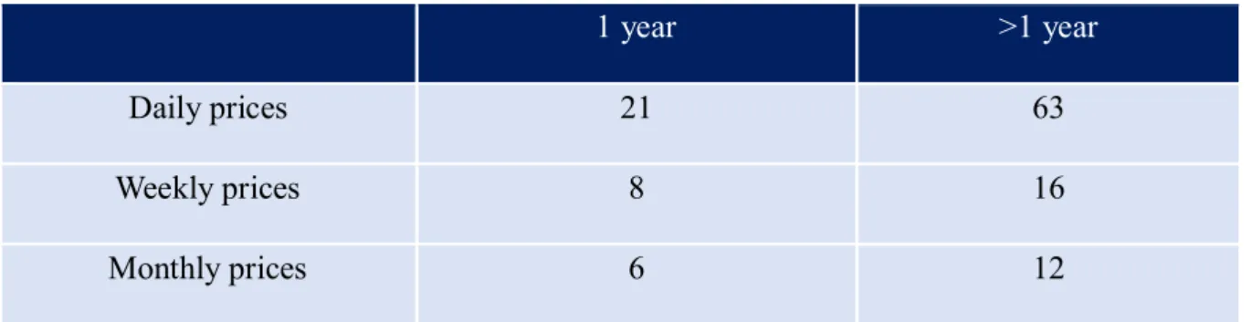
The evaluation of the stress scenario is different from the other ones and requires additional sub-calculations. The first step is identifying an appropriate length of the sub-interval (different for the recommended holding periods 1, 3, and 5 years), according to the table provided:

1 year >1 year

Daily prices 21 63

Weekly prices 8 16

Monthly prices 6 12

Figure 2 - Length of the sub-intervals

Two approaches have been dominant in this area.

Approach 1

For the observations of the prices use the intervals to construct subsets of the prices, for each:

𝑖 = 1,2, … , 𝑀 − 𝑥 + 1

, where the price set:

{𝑃

_𝑖

, 𝑃

_𝑖+1

, … , 𝑃

_{𝑖+𝑤−1}

}

, contains exactly 𝑤 elements. This interval corresponds to 𝑤-1 observed returns:

{𝑟

_𝑖+1

, 𝑟

_𝑖+2

, … , 𝑟

_{𝑖+𝑤−1}

}

Approach 2

For the observations of the prices use the intervals to construct subsets of the prices, for each:

(19)

19 , take the price set:

{𝑃

_𝑖

, 𝑃

_𝑖+1

, … , 𝑃

_𝑖+𝑤+1

}

, which contains “𝑤 + 1” elements. This interval corresponds to 𝑤 observed returns:

𝑟

_𝑖+1

, 𝑟

_𝑖+2

, … , 𝑟

_𝑖+𝑤

The main difference is driven by only one observation. However, in the case of weekly and monthly data for the first year it is a considerable influencer. For the scope of this report, it has been decided to extend the number of observations and adapt the second methodology.

Following that, the formula used in the rolling volatility calculations is:

𝜎

_𝑆

𝑖

𝑤

_{= √}

∑

𝑖+𝑤𝑗=𝑖

(𝑟

𝑗

−

𝑖+𝑤𝑖

𝑀

1

)

2

𝑀

_𝑤

, where:

𝑀𝑤 - is the count of the number of observations in the sub-interval (equal to 𝑤),

𝑀1 𝑖

𝑖+𝑤 _{= 𝐴𝑣𝑔(}_𝑟

𝑖+1, 𝑟𝑖+2, … , 𝑟𝑖+𝑤) – is the mean of all the historical lognormal returns in the

corresponding sub-interval.

From these volatilities, the stressed volatility is calculated by taking the value that corresponds to the 99th percentile for the first year and the 90th percentile for the following holding periods (3 and 5 years). The stressed volatility is denoted by:

𝜎

𝑆 𝑤

The formula for the Stressed Scenario is as follows:

𝑆𝑡𝑟𝑒𝑠𝑠

_{𝑆𝑐𝑒𝑛𝑎𝑟𝑖𝑜}

= 𝑒

𝑘 , where:

𝑘 = 𝜎

𝑤 _𝑆

√𝑁 (𝑍

𝛼

+ (

𝑧𝛼 2₋₁ 6

)

𝜇1 √𝑁

+ (

𝑧𝛼3−3𝑧𝛼 24

)

𝜇2 𝑁

− (

2𝑧𝛼3−5𝑧𝛼 36

)

𝜇12 𝑁

) − 0,5 𝜎

𝑆2

𝑁

𝑤 .

(20)

20 From this formula, it can be deduced that the skewness and the kurtosis used, are the ones taken from the entire distribution of returns since there is no subscript in 𝜇₁ and 𝜇₂ that indicates a rolling skewness and kurtosis.

These figures and disclosures required in the KIDs are not always clear and could misguide the investors. Particularly, the figures related to the performance scenarios can be easily misinterpreted.

First of all, as previously mentioned, the performance scenarios are based on past data, which consist of funds’ historical prices. Usually, through a time series of 5-year prices, the potential amounts and the potential returns are predicted, for 3 different future time periods.

However, a structure which bases the computation of future data exclusively on past data, cannot be totally accurate. Indeed, if the past returns of a certain fund were positive for all the time series taken into consideration, the performance scenarios will be as well positive. The opposite is true; if the last 5 years’ data are negative, then the prediction related to the performance scenarios will be very pessimistic.

Consequently, the results related to the scenarios could be inaccurate and couldn’t help investors in making more informed investment decisions: the scenarios and the actual returns of the investment product could mismatch.

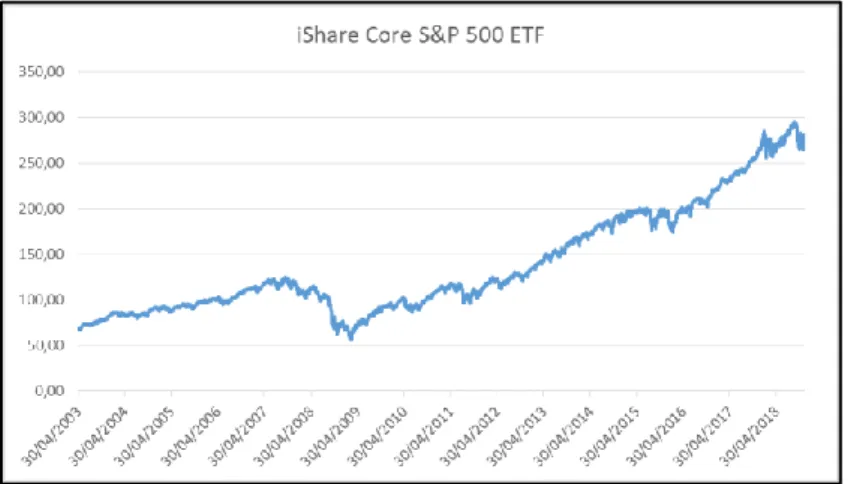
As an example, it has been considered the iShare Core S&P 500 - IVV, an ETF exposed to large American firms, which tracks the S&P 500 index. Particularly, the analysis wants to highlight the difference between the potential results that investors would have obtained according to performance scenarios in 2008, and the actual score they gained in reality.

As it is shown in the figure below, which represents the historical prices, the ETF is characterized by an increasing trend from 2003 until the beginning of 2008. The spike that follows this period is due to the financial crisis.

(21)

21 Figure 3 – IVV historical prices values

Therefore, it has been assumed an investor could have invested 10.000 dollars in this product in January 2008, with a recommended holding period of 5 years. According to the performance scenarios methodology, collecting 1.261 daily prices form 2003 until 200818_{to obtain 1.260}

observations in terms of LN returns (= 5 years * 252 working days), after one year (2009), the

investment would have given back a return of almost 30% in the best scenario and a return of -14,48% in the worst case (see the figure below).

Performance scenarios

11 33 5

Unfavourable scenario amount 10.099,350 9.955,385 11.074,685

Unfavourable scenario return 0,10% -0,15% 2,06%

Moderate performance amount 11.007,060 13.328,085 16.138,537

Moderate performance return 10,07% 10,05% 10,05%

Favourable scenario amount 13.016,244 17.826,786 23.495,924

(22)

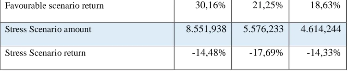
22

Favourable scenario return 30,16% 21,25% 18,63%

Stress Scenario amount 8.551,938 5.576,233 4.614,244

Stress Scenario return -14,48% -17,69% -14,33%

Figure 4 – IVV performance scenarios values

However, the actual annual return at the beginning of 2009 was around -24% since, as illustrated in Figure 3, the prices values significantly decreased in a very short time (the return has been computed through the collection of 253 daily prices from 2008 until 2009, the calculation of 252 LN returns, and then, the computation of the annual average return for that period).

In 2011 (2nd_{period) the actual return was more close to the scenarios’ results, due to the increase}

in the ETF prices and was around 12% (the actual return has been computed through the collection of 757 daily prices from 2008 until 2011, the calculation of 756 LN returns, the computation of the annual average return for that period), while in 2013 the high values reached by the product led to an annual return of 47% (the actual return has been computed through the collection of 1.261 daily prices from 2008 until 2013 (3rd_{period), the calculation of 1.260 LN}

returns, the computation of the annual average return for that period).

Through this example, it can be said that the PRIIPs performance scenarios are not always an accurate disclosure of the potential risks and returns. On one hand, none of the scenarios, even the stress scenarios, is not able to capture the severe effects of an unexpected crisis; on other hand, the favourable scenario is not able to capture possible significant increase of the investment values. In reality, the markets are affected by shocks (both positive and negative) that the PRIIPs methodology often cannot predict. In this way, investors could be misguided and could choose the “wrong” investment product, since they are not concerned of the real risks related to it.

(23)

23 Consequently, “past data are not always good representation of future results”.

Another example that supports this statement, is the analysis below.

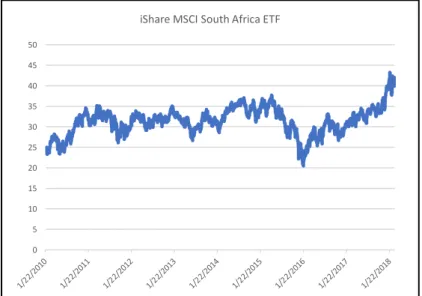
A general ETF, not related to an index which suffered the crisis, the iShare MSCI South Africa ETF, has been taken into consideration. This specific fund is characterised by a high volatility. For this product, daily prices have been collected from 2010 until 201819_{. Furthermore, it is}

assumed an investment in each product in 2015 and a recommended holding period of 5 years (i.e. the first period ends in 2016, the second in 2018 and the third one, in 2020). The performance scenarios have been calculated using 1.261 data from 2010 until 2015 to obtain 1.260 observations in terms of LN returns (= 5 years * 252 working days).

Performance Scenarios

Rec. Holding Periods In Years 1 3 5

N 252 756 1260 Interval Length (W) 21 63 63 Percentile 1% 5% 5% Z alpha -2,326 -1,645 -1,645 WϬs (Stressed Volatility) 0,031 0,023 0,023 Unfavourable Scenario 0,748 0,638 0,588 Moderate Scenario 1,044 1,137 1,239 Favourable Scenario 1,457 2,028 2,615 Stressed Scenario 0,288 0,287 0,185

Figure 5 – MSCI SA performance scenarios values

(24)

24 As it is shown in the table above, at the end of the first period, a certain investor could get back from this product a value of 0,748 for the unfavourable scenario; 1,044 for the moderate scenario; 1,457 for the favourable scenario and 0,288 for the stress scenario (these values should be then multiplied by 10.000 which is assumed to be the amount invested in the product). Although, the actual annual value in 2016, which is approximately 0,56 (the value has been computed through the collection of 253 daily prices from 2015 until 2016, the calculation of 252 LN returns, and then, the computation of the exponential value of the annual average return for that period), is not corresponding to any of the scenarios results. The same is true in the second period (2018) since the historical value is almost 1,4 (the value has been computed through the collection of 757 daily prices from 2015 until 2016, the calculation of 756 LN returns, and then, the computation of the exponential value of the annual average return for that period) due to changes in prices, not taken into consideration within the scenarios’ results, as shown in Figure 4.

Figure 6 – MSCI SA historical prices values

In general, it can be said that, the PRIIPs methodology is not always able to capture the high volatility, and therefore, to give a full and complete understanding of the investment proposed.

0 5 10 15 20 25 30 35 40 45 50

(25)

25 Indeed, the retail investor should take the results given by the scenarios, only as an approximation and an indication of the future performance and should consider this while taking investment decisions.

A solution to this problem could be the introduction of the Montecarlo simulation. Indeed, the method has an important role in the stochastic simulation and is already widely used as a technique to assess the investment risk. Particularly, the Montecarlo simulation, assuming that the future cash flows are related to stochastic variables, could indicate the entire probability distribution of the output (e.g. potential returns), and not just a point estimate. This would also allow measuring the risk- and the reward profile of the investment project through a statistical dispersion. The elements needed for the method are 4:

- Parameters, (i.e. specific inputs as the prices of the product/investment);

- Exogenous shocks (i.e. input that cannot be predicted, but can be defined in terms of probability, as the shock in prices);

- Outputs (i.e. simulation results, as the returns that the investor could get back by investing in a certain product/investment);

- Model (i.e. mathematical equations that could describe the relationship between the outputs, the inputs, and the parameters).

The results would be more accurate compared to the actual performance scenarios, but it should be said that it would be not easy to set-up the method within a database such as SQL, and this is the reason why companies like EY Luxembourg have not implemented this for the Category 2 of PRIIPs.

However, the projection through past data is not the only shortcoming related to the PRIIPs performance scenarios. Indeed, these can be misleading in different ways.

(26)

26 For the analysis two funds are considered. The related prices have been collected from 2013 until 2017. Fund 1 has an annual volatility of 0,005739, while Fund 2 has an annual volatility of 0,006583, as shown in the figures below.

M1 -1,9E-06

Volatility 0,005739

Skewness -14,4506

Excess kurtosis 372,36

Figure 7 – Fund 1 statistical measures Figure 8 – Fund 2 statistical measures

Even if the volatility of Fund 1 is lower than the volatility of Fund 2, the potential return that the investor could get back in the stress scenario after 1 year would be worst if he/she would invest in the first fund. As presented in Figure 7, the return the investor would receive, would be -83,58% for Fund 1 and, as clearly shown in Figure 8, it would be higher if he would invest in Fund 2, since the return would be -41,14%.

Performance scenarios

Unfavourable scenario amount 8.825,17 8.011,07 7.479,27

Unfavourable scenario return -11,75% -7,13% -5,64%

Moderate performance return 0,92% 0,00% -0,19%

Favourable scenario amount 11.029,45 11.927,68 12.541,71

Favourable scenario return 10,29% 6,05% 4,63%

M1 0,000218

Skewness -0,82411

(27)

27 Figure 9 – Fund 1 performance scenarios values

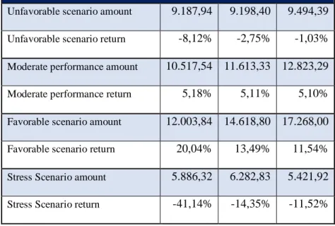
Performance scenarios

Unfavorable scenario amount 9.187,94 9.198,40 9.494,39

Unfavorable scenario return -8,12% -2,75% -1,03%

Moderate performance return 5,18% 5,11% 5,10%

Favorable scenario amount 12.003,84 14.618,80 17.268,00

Favorable scenario return 20,04% 13,49% 11,54%

Figure 10 – Fund 2 performance scenarios values

The reason behind this mismatching between volatility and scenarios’ results can be found in the past performance: as the two figures below show, Fund 1 has a spike (i.e. significant decrease in price on the 15/01/2015). Indeed, as previously specified, the stressed volatility is computed by taking the value that corresponds to the 99th percentile scenario; this means that the spike is captured and over-weighted, leading to worst performance scenario at the end of the first year for Fund 1, compared to Fund 2.

(28)

28 Figure 11 – Fund 1 historical prices values

Figure 12 – Fund 2 historical prices values

A solution could be the inclusion of the past performance in the form of past prices within the performance scenarios’ section. Therefore, the retail investor would have more information about a certain investment/product. He/she could have a better overview on the trend of the different products and indeed, he could take a more accurate investment decision.

The disclosure of the past performance would also be important for investors in other cases. For the analysis two funds are considered. The related prices have been collected from 2014 until 2018.

(29)

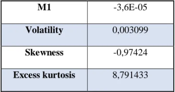
29 Fund 3 and Fund 4 have the same statistical measures (mean, volatility, skewness and excess kurtosis), as shown in the figures below.

M1 -3,6E-05

Skewness -0,97424

Excess kurtosis 8,791433

Figure 13 – Fund 3 statistical measures Figure 14 – Fund 4 statistical measures

This would lead to the case in which the two funds have approximately the same performance scenarios, as shown in Figures 13 and 14.

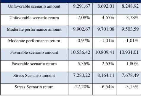
Performance scenarios

Moderate performance return -0,97% -1,01% -1,01%

M1 -3,6E-05

Skewness -0,97424

(30)

30

Performance scenarios

Moderate performance return -0,97% -1,01% -1,01%

As a result, an investor could be indifferent between Fund 3 and Fund 4.

(31)

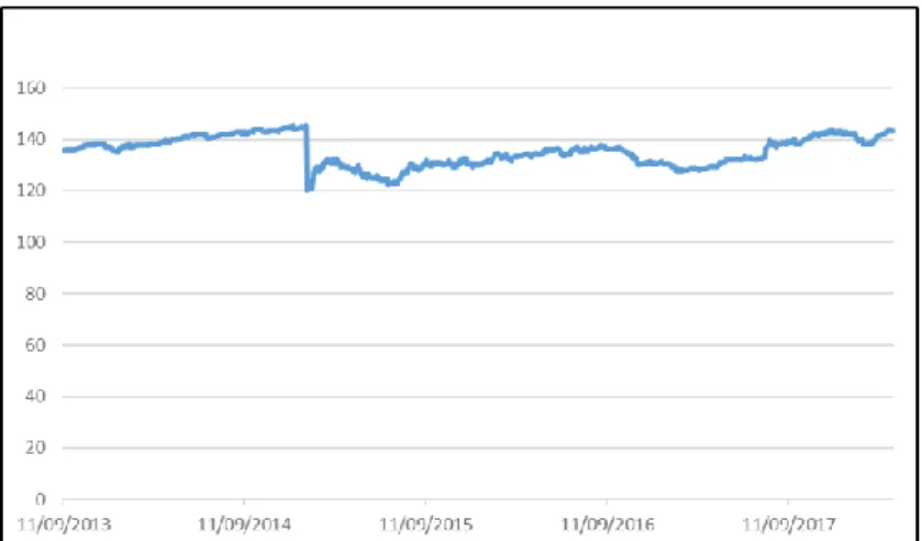
31 Figure 18 – Fund 4 historical prices values

However, as it is clearly shown in the figures above, the funds have two opposite past performance trends, in terms of past prices. This would be an important information that could affect the investors’ decisions and could increase the level of comparability among investment products.

(32)

32

3. Conclusion

As a response to the crisis, the ESAs have improved many regulations, such as PRIIPs, to increase transparency and allow an investor to take a better investment decision.

However, there are some shortcomings in the regulation. Particularly, as shown in the examples above, the performance scenarios’ figures could be misleading.

The 8th on November 2018, the ESAs have published a paper20_{, proposing several changes for}

the PRIIPs KID, with a focus on the scenarios.

Among these, there is the inclusion of the past performance, since it became clear how the disclosure of historical trends could help investors. EY Luxembourg is planning to include the products’ price trends within the performance scenarios’ section, and, if available, also the related benchmark trends. This would allow its clients to have a better overview of a certain product/investment. Furthermore, the company is working to set in a proper way the Montecarlo simulation for PRIIPs Category 2 within the SQL database, to limit the problems related to the past data for the performance scenarios’ calculation.

The ESAs would include the changes before the end of 2019 within the PRIIPs regulation, and particularly, within the KIDs to increase the transparency and the level of comparability among different products, so that investors would have a more accurate perception of the risks related to these instruments.

(33)

33

4. References:

- Regulation (EU) No 1286/2014 of the European Parliament and of the Council of 26 November 2014 on key information documents for packaged retail and insurance-based investment products (PRIIPs), available at: https://eur-lex.europa.eu/legal-content/EN/TXT/PDF/?uri=CELEX:32014R1286&from=en

- Commission Delegated Regulation (EU) 2017/653 of 8 March 2017 supplementing Regulation (EU) No 1286/2014 of the European Parliament and of the Council on key information documents for packaged retail and insurance-based investment products (PRIIPs) by laying down regulatory technical standards with regard to the presentation, content, review and revision of key information documents and the conditions for fulfilling the requirement to provide such documents, available at: https://eur-lex.europa.eu/legal-content/EN/TXT/PDF/?uri=CELEX:32017R0653&from=EN

- Anna Maria Tarantola, “Verso una nuova regolamentazione finanziaria”, Italy, 2011, available at: https://www.bancaditalia.it/pubblicazioni/interventi-direttorio/int-dir-2011/tarantola_210111.pdf

- Commissione Nazionale per la Società e la Borsa (CONSOB – Autorità italiana per la vigilanza dei mercati finanziari), “La crisi finanziaria del 2007-2009”, available at: http://www.consob.it/web/investor-education/crisi-finanziaria-del-2007-2009

- Jerard Caprio, Jr, “Financial Regulation After the Crisis: How Did We Get Here, and How Do We Get Out?”, 2013, available at: http://www.lse.ac.uk/fmg/assets/documents/papers/special-papers/SP226.pdf

(34)

34 - Caroline Bradley, “Transparency and Financial Regulation in the European Union: Crisis and Complexity”, 2017, available at: https://ir.lawnet.fordham.edu/cgi/viewcontent.cgi?referer=http://www.google.co.uk/ur l?sa=t&rct=j&q=&esrc=s&source=web&cd=5&ved=2ahUKEwiqg4fJ09XdAhVDBy wKHTLeAagQFjAEegQIAhAB&url=http%3A%2F%2Fir.lawnet.fordham.edu%2Fcg i%2Fviewcontent.cgi%3Farticle%3D2596%26context%3Dilj&usg=AOvVaw2QJrHnj Ei3I_9OPHPdE1pb&httpsredir=1&article=2596&context=ilj

- Vincenzo d’Apice, Giovanni Ferri, “Instabilità economica globale: crisi e regole della Finanza”, Carocci Editore, 2011.

- Risk Management Solutions, “Anatomy of Cornish – Fisher”, 2016, available at: http://www.riskconcile.com/rc/rd/CornishFisher02.html

- Giulio Aquino, Francesco Rossi, Matteo Tesser, “Packaged Retail Investment and Insurance-based Investments Products (PRIIP) - Scenari di performance con traiettorie

alla Cornish-Fisher”, available at:

(35)

35 - European Fund and Asset Management Association (EFAMA), “EFAMA’s evidence on the PRIIP KID’s shortcomings”, 2018, available at: https://www.efama.org/Publications/Public/PRIPS/184008_EFAMAPRIIPsEvidenceP aper.pdf

- Ettore Bolisani, Roberto Galvan, “La simulazione Montecarlo: appunti integrativi”, available at: http://static.gest.unipd.it/labtesi/eb-didattica/EAI/montecarlo

- ESAs “Joint Consultation Paper concerning amendments to the PRIIPs KID”, draft amendments to Commission Delegated Regulation (EU) 2017/653 of 8 March 2017 on key information documents (KID) for packaged retail and insurance-based investment products (PRIIPs).

(36)

36

5. Annex

(37)

(38)

38