Scientific Annals of Economics and Business 66 (4), 2019, 465-486
DOI: 10.2478/saeb-2019-0043
Price Clustering in Bank Stocks During the Global Financial Crisis
Júlio Lobão* , Luís Pacheco** , Luís Alves***Abstract
Market anomalies are one of the most intriguing and fascinating phenomena observed in financial markets. This paper examines the incidence of price clustering in US and European bank stocks during the Global Financial Crisis. The results reveal a significant level of price clustering in European and US banks’ samples, which is difficult to reconcile with the Efficient Market hypothesis. The Attraction hypothesis and the Price Resolution/Negotiation hypothesis seem to be the best explanations for the clustering effect. However, the results also suggest that the uncertainty associated with the crisis did not have a significant impact in the clustering levels, which is at odds with the recently proposed Panic Trading hypothesis. Surprisingly, we observe a tendency to have less price clustering during the period of crisis and banks located in countries mostly affected by the European sovereign debt crisis exhibit lower levels of price clustering. These results are consistent with the idea that investors tend to be more analytical in their appraisals in periods of negative sentiment.
Keywords: price clustering; financial crisis; behavioral finance; sovereign debt crisis; banking industry. JEL classification: G12; G14; G01; G4.
1. INTRODUCTION
Market anomalies are one of the most intriguing and fascinating phenomena observed in financial markets. One of the most studied issues over the last decades has been price clustering, with the first evidence published in the 1960s (Osborne, 1962). The Efficient Market hypothesis posits that prices should follow a random walk and fully reflect all available information. Being prices in theory the reflection of the assets’ fundamental value, there is no apparent reason to observe an accumulation of prices in certain levels or numbers. However, there is extensive evidence showing that certain prices are traded more frequently than others (Niederhoffer, 1965; Harris, 1991; Mitchell, 2001; Ikenberry and Weston, 2008).
*
School of Economics and Management, University of Porto; CEPESE – Centro de Estudos de População, Economia e
Sociedade; Portugal; e-mail: [email protected] (corresponding author).
**
Department of Economics and Management, Portucalense University; REMIT – Research on Economics,
Manage-ment and Information Technologies; IJP – Portucalense Institute for Legal Research; Portugal; e-mail: [email protected].
***
The debate on the determinants of price clustering is still ongoing. Stock price clustering was found to depend on variables such as price level, idiosyncratic volatility, firm size, trade size, transaction frequency and liquidity (Christie et al., 1994; Aitken et al., 1996). More recently, Narayan and Smyth (2013) proposed the "panic trading hypothesis" according to which when investors are in a period of heightened stress they tend to quickly settle on a rounded price in order to avoid selling at a lower price at a later moment. Therefore, prices should exhibit higher levels of clustering in those circumstances. Narayan and Smyth (2013) found support for the panic trading hypothesis in their case study about the Fiji’s stock market. However, to date, to the best of our knowledge, there has been no other test on the panic trading hypothesis. In this paper we fill this gap by conducting a study on the impact of financial instability associated with the Global Financial Crisis on the incidence of price clustering in the US and European bank stocks.
Overall, the results show significant levels of price clustering in bank stocks. However, the financial crisis does not seem to have had a significant impact on the observed levels of clustering. On the contrary, our results reveal a tendency to lower levels of price clustering in the crisis period. In addition, our cross-sectional analysis shows that price clustering was negatively associated with liquidity in both the US and European bank stocks.
This paper is structured as follows: the 2nd Section presents a literature review and the 3rd Section describes the data and methodology. The 4th Section analyzes the results and, finally, the 5th Section exposes the main conclusions.
2. LITERATURE REVIEW
2.1 Definition and main hypotheses behind price clustering
The concept of price clustering originates from the studies of Osborne and Niederhoffer published in the 1960s. Osborne (1962) presented evidence of a tendency for certain share prices to spend an inordinate amount of time at a certain price range. In an efficient market, prices should be uniformly distributed and price clustering should not exist (Niederhoffer, 1965; De Grauwe and Decupere, 1992; Aitken et al., 1996). Assuming that the price of an asset is nothing more than the reflection of its intrinsic value, in the absence of market frictions there would be no reason for certain prices to be observed more frequently than others.
Mitchell (2001) suggested some reasons for the emergence of this phenomenon. One of these conditions is the dominance of a certain market by a small number of investors, which makes it difficult for a certain biased behavior to be eliminated of the market. Other reasons pointed out include the existence of trading impediments that prevent the observance of some values, the generalized preference of the market participants for certain numbers and the existence of biases in the decision-making environment. One or more of these conditions would be sufficient for that trading behavior to be reflected in an empirically observable phenomenon. Alternatively, P. Brown and Mitchell (2008) defined price clustering as the concentration of stock prices on some numbers rather than others as a result of human bias, imprecise beliefs or haziness about the underlying value of a security.
The literature presents five main hypotheses to explain price clustering: the Price Resolution hypothesis, the Negotiation hypothesis, the Attraction hypothesis, the Collusion hypothesis, and the Panic Trading hypothesis.
The Price Resolution hypothesis (Ball et al., 1985) states that the uncertainty about the intrinsic value of a given security causes market participants to use coarser price grids, which in turn generates price clustering. This hypothesis also suggests that the degree of price resolution is related to the amount of information available in the market. For example, larger companies that are followed by a large number of financial analysts should have a higher level of information. This will allow for a larger price set and lower levels of clustering. On the other hand, the level of price resolution should be negatively related to the price level since the higher the value of an asset, the greater the tendency for market participants to use a coarser price grid. Stock price volatility is also expected to impact the clustering level as volatility can be understood as a reflection of the uncertainty regarding the intrinsic value of a given asset. Moreover, a higher level of trading liquidity can be associated to a higher level of information and thus less clustering. In short, the lower the quantity and quality of information in the market, the greater the uncertainty; the lower the level of price resolution and more likely price clustering will be observed.
According to the Price Negotiation hypothesis (Harris, 1991), one should observe greater clustering when the negotiation costs are larger. That is the case, for example, for high volume transactions, when the market, industry or firm are characterized with greater volatility or when the price level is high. Harris (1991) argues that price clustering occurs because investors use discrete price sets as a mechanism to reduce the cost of negotiating transactions. In periods of abnormally heavy trading, as is the case of periods of crisis, where uncertainty levels soar, the need to execute trades quickly and with the least possible cost leads market participants to reduce their terms of trading. By using a coarser price grid, individuals are reducing the amount of information that has to be processed, making transactions to occur more swiftly, as bid and offer prices converge more rapidly. In summary, the negotiation hypothesis states that prices cluster at round numbers to reduce negotiation costs and time to make a deal during transactions.
The Attraction hypothesis proposed by Curcio and Goodhart (1991) suggests that there is a natural tendency for individuals to feel more attracted to certain numbers rather than others without any apparent rational motivation, creating clustering in certain price points. Several studies on the Attraction hypothesis have concluded that in a decimal system, transaction prices ending in zero are more often observed because this number is more salient. After 0, the 5 is the stronger attracter, followed by the even numbers 2 and 8. The 1 and 9 are the least observed digits because there will be a natural attraction for 0 (the most observed digit). The relative frequency of 3 will be the same as 7. The same can be said for 4 and 6. However, there is no clear evidence as to which of these groups, {3 = 7} and {4 = 6} should be more common, depending on the "gravitational pull" of the 5 in relation to the adjacent even numbers and the preference of the individuals for even rather than odd numbers.
The Collusion hypothesis was firstly suggested by Christie et al. (1994), arguing that traders intentionally collude to set non-competitive bid-ask spreads. The authors show that the structure of multiple dealers in the NASDAQ market leads to an incentive to maintain non-competitive bid-ask spreads through an agreement to avoid odd eight quotes, thus resulting is an increase in their profit margins per transaction and price clustering.
Finally, Narayan and Smyth (2013) proposed the Panic Trading hypothesis. The hypothesis states that in a period of heightened market uncertainty investors should be more prone to settle quickly on a rounded price to avoid having to sell at a lower price at a later moment. Therefore, one expects to observe a higher incidence of price clustering in those
circumstances. Narayan and Smyth (2013) found that political instability in Fiji triggered price clustering behavior thus confirming the Panic Trading hypothesis.
2.2 Previous empirical evidence
Osborne (1962), Niederhoffer (1965), Harris (1991) and Christie et al. (1994) were among the first to study the microeconomics of price formation and to document that US prices cluster around whole numbers and common fractions.
Aitken et al. (1996) documented the existence of price clustering in equity markets out-side the US that used decimal trading rather than fractions. The authors analyzed the last digit of individual trade prices on the Australian Stock Exchange (ASE) using intraday transaction data. The results confirmed the Price Resolution hypothesis, but also showed evidence in favor of the Attraction hypothesis, with prices ending in 0 being the most preferred, followed by prices ending in 5 and even digits. Clustering increased with the market-wide volatility, own stock volatility, price level, trade size and the size of the bid-ask spread. Unlike Harris (1991), their results showed greater clustering for larger firms. In addition, they were able to observe in their sample a lower level of clustering for shares with options traded on them, for stocks in which short selling was allowed and in more liquid stocks.
Hameed and Terry (1998) studied price clustering in limit orders in the Singapore Stock Exchange, a fully electronic order-driven market. The authors found clustering at all price ranges, with whole dollars being more frequent than half dollars, which in turn were more often observed than prices ending in multiples of 10 cents. After this, in descending order of frequency, prices ending in odd-multiples of 5 cents were the most observed. The authors found support for the Negotiation hypothesis, with clustering increasing with price level and decreasing with trading volume, despite their findings showed no consistent relationship between clustering and stock price volatility.
P. Brown et al. (2002) were the first to study the impact of cultural factors on price clustering, analyzing six Asia-Pacific stock markets and concluding for the pervasiveness of stock price clustering in all markets. Thus, the authors found evidence supporting both the Price Resolution and the Attraction hypotheses. Moreover, cultural factors were shown not to have a significant influence on clustering.
Ohta (2006) investigated price clustering on the Tokyo Stock Exchange with intraday data. His results were consistent with the Price Resolution hypothesis. Price clustering seemed to be higher just after the market opening when the level of uncertainty is higher. However, Aşçıoğlu et al. (2007), using quotes from the same exchange, only found limited support for the Price Resolution hypothesis and concluded that this anomaly was best explained by the Attraction theory.
Ikenberry and Weston (2008), in their study on the impact of decimalization on price clustering, found evidence in support of the Negotiation and Price Resolution hypotheses. Adopting a different approach, Blau and Griffith (2016), tested the hypothesis that clustering in round pricing increments would result in more volatile financial markets, since stocks with a greater degree of clustering will have less informative prices. The authors evidenced that causation flows from clustering to volatility instead of the other way around.
Regarding the Collusion hypothesis, Huang and Stoll (1996) concluded that collusion in a multiple dealer market with easy entry is extremely unlikely to occur. On the contrary, Aşçıoğlu et al. (2007) analyzed the Tokyo Stock Exchange, where trading takes place
electronically without market markers, so explicit collusive behavior could not exist and still found evidence of price clustering.
More recently, Das and Kadapakkam (2018) examined time trends in price clustering for Exchange-Traded Funds (ETFs) and individual stocks, evidencing a substantial reduction in clustering over the sample period (2001-2010). The authors attributed that to the increasing proeminence of algorithmic trading, which seems to be less susceptible to psychological biases.
Different studies evidenced the existence of price clustering in other asset classes such as exchange rates (Curcio and Goodhart, 1991; Sopranzetti and Datar, 2002), initial public offerings and seasoned equity offerings (Kandel et al., 2001; Mola and Loughran, 2004; Hu et al., 2019), commodities (Bharati et al., 2012; Palao and Pardo, 2012), derivatives (ap Gwilym et al., 1998; Narayan et al., 2011), betting markets (A. Brown and Yang, 2016), and cryptocurrencies (Urquhart, 2017; Baig et al., 2019). These papers presented evidence supporting the different hypotheses, underlining the empirical nature of this issue. For instance, Kandel et al. (2001) and Narayan et al. (2011) supported the Attraction hypothesis, whereas ap Gwilym et al. (1998) found only limited evidence for this explanation, preferring the Price Resolution hypothesis and Mola and Loughran (2004) and Hu et al. (2019) both provided support for the Negotiation hypothesis.
3. DATA AND METHODOLOGY 3.1 Data
The present paper uses daily closing prices from two samples, one with US bank stocks and the other with bank stocks from nine European countries (Austria, Denmark, Finland, Germany, Greece, Italy, Portugal, Romania and Spain), with a different crisis period for each one. Following Davis et al. (2009), we define the crisis period for the US banks’ sample as the period from October 9, 2007 to March 9, 2009. Regarding the sample of European banks, we follow Attinasi et al. (2009) to define the European crisis period as the period between July 31, 2007 and March 25, 2009. To set the periods before the crisis, we use a range of 24 months before each of the periods defined above. All data were obtained from Thompson Reuters DataStream.
3.2 Univariate analysis
We will carry out a univariate analysis of the frequency with which the last digit of the stock prices is observed. According to the null hypothesis of non-existence of price clustering, it is expected a frequency of 0.10 for each digit. Following Ikenberry and Weston (2008), we then apply an adaptation of the Herfindahl-Hirschman-Index (HHI) to measure price clustering. This index is usually used to assess market concentration, but in this case it will be used to measure the concentration of prices and how different it is from a uniform distribution. The statistic will be computed by adding the squared values of the percentage of prices ending in certain digits, that is:
HHI = ∑(fi)2 B
i=1
where fi is the frequency (in percent) of closing stock prices that occur at fractions i=1,2,…B possible bins. If there was no price clustering, HHI should be equal to 1/10 = 0.1, since each digit would have a frequency of 10%. In the case of perfect price clustering, where prices are concentrated entirely on a single digit, HHI would equal unity. In order to compare the price clustering between the two periods under analysis, before and during the crisis, and to determine whether the level of price clustering actually changed in the financial crisis period, this paper uses two frequently used statistics in this kind of analysis (Ikenberry and Weston, 2008; Palao and Pardo, 2012). First, to test the significance of price clustering in a given sample over a given period, it is used the standard Chi-square goodness-of-fit statistic that, according to the null hypothesis (hypothesis H1, from now on) of absence of difference between the observed distribution and the expected uniform distribution should be below some critical value. We define this statistic, D, as follows:
D = ∑(Oi− Ei) 2 Ei N i=1 (2)
where Oi is the observed frequency of observations in bin i = 1,…, N and Ei is the expected frequency of observations under the null uniform distribution. D has a Chi-square distribution with N-1 degrees of freedom under standard regularity conditions. A larger value of D would signify a deviation from the expected distribution, thus implying price clustering.
After this first step, we use the following statistic to compare the level of price clustering between the two periods under analysis and between subsamples:
D ̃ = (D2
D1) ~ FN2−1,N1−1 (3)
where 𝐷𝑖 ~ 𝜒𝑁−12
Under the null hypothesis (hypothesis H2, from now on), the two samples considered are equally clustered. We use this statistic to test the hypothesis that the level of price clustering has changed between the periods before (D1) and during the financial crisis (D2)
for each subsample. Higher values of D̃ would mean a significantly higher level of clustering in one of the subsamples.
3.3 Multivariate analysis
The multivariate analysis is used to determine which variables can explain price clustering at the firm level. Regarding the dependent variable, we follow Ikenberry and Weston (2008) to estimate the level of price clustering at the firm level considering all closing prices over the sample period. Thus, we will consider the difference between the HHI measure and the level of clustering that would be expected under the null hypothesis, that is, a HHI value of 0.1.
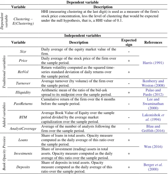
The independent variables included in our analysis are expected to capture the firm characteristics that may impact on clustering levels. Each independent variable is log-transformed and standardized to have a zero mean and unit variance. The different variables are described below and Table no. 1 presents the description of the variables as well as their expected signs.
Thus, the following model is estimated using OLS: 𝐶𝑙𝑢𝑠𝑡𝑒𝑟𝑖𝑛𝑔 − 𝐸(𝐶𝑙𝑢𝑠𝑡𝑒𝑟𝑖𝑛𝑔) = 𝛼 + 𝛽1𝑆𝑖𝑧𝑒 + 𝛽2𝑃𝑟𝑖𝑐𝑒 + 𝛽3𝑅𝑒𝑡𝑣𝑜𝑙 + 𝛽4𝑇𝑢𝑟𝑛𝑜𝑣𝑒𝑟 + 𝛽5𝐼𝑙𝑙𝑖𝑞𝑢𝑖𝑑𝑖𝑡𝑦 + 𝛽6𝑃𝑎𝑠𝑡𝑅𝑒𝑡𝑢𝑟𝑛𝑠 + 𝛽7𝐵𝑇𝑀 + 𝛽8𝐴𝑛𝑎𝑙𝑦𝑠𝑡𝐶𝑜𝑣𝑒𝑟𝑎𝑔𝑒 + 𝛽9𝐿𝑜𝑎𝑛𝑠 + 𝛽10𝐼𝑛𝑣𝑒𝑠𝑡𝑚𝑒𝑛𝑡𝑠 + 𝛽11𝐷𝑒𝑝𝑜𝑠𝑖𝑡𝑠 + 𝛽12𝑆𝑖𝑧𝑒𝐴𝑠𝑠𝑒𝑡𝑠𝐵𝑉 + 𝛽13𝑇𝑜𝑏𝑖𝑛𝑄 + 𝛽14𝐶𝑟𝑒𝑑𝑖𝑡𝑅𝑖𝑠𝑘 + 𝛽15𝑅𝑂𝐴𝑉𝑂𝐿 + 𝛽16𝑁𝐼𝑀𝑉𝑂𝐿 + 𝛽17𝑍𝑆𝐶𝑂𝑅𝐸 (4)
The variables that capture average size (“Size”), average price (“Price”), return volatility (“RetVol”), average turnover (“Turnover”) and liquidity (“Illiquidity”) are usually included in the studies about price clustering (e.g., Harris, 1991; Ikenberry and Weston, 2008). According to the Price Resolution/Negotiation hypotheses larger firms tend to display a higher level of information than smaller firms, so a negative relation between the size factor and the level of clustering should be expected. Moreover, those hypotheses also suggest that the stock price has a highly significant explanatory power in the variation of the level of price clustering, and it is expected that as the price level increases, the "minimum tick size" will gradually become a smaller percentage of the share’s value, leading investors to use a coarser price grid. It should also be expected that greater volatility of returns generates greater uncertainty about the value of stocks and that this uncertainty will lead investors to round prices, creating price clustering. Regarding the variable “Turnover”, the Price Resolution hypothesis suggests that banks that present a higher turnover should exhibit a lower level of clustering. Also, the greater the liquidity of a stock, the lower should be the level of clustering, since prices tend to be known with a higher degree of precision.
The variable “PastReturns” is expected to have a negative relation with price clustering, since higher returns in the past should lead to an increased attention and coverage by both investors and analysts (Lee and Swaminathan, 2000), which in turn should decrease the level of uncertainty about the stock price. In theory, growth stocks (captured by the variable “BTM”) should be more affected by clustering. As pointed out by Lakonishok et al. (1994), this type of stocks tends to attract naïve investors whose biases might lead to clustering in prices. Following Blau and Griffith (2016), we expect that a higher number of analysts (“AnalystCoverage”) covering a stock will lead to less uncertainty and, consequently, less price clustering.
The model also includes three variables (“Loans”, “Investments” and “Deposits”) that intend to capture bank’s opacity, since more opaque banks should exhibit a higher degree of price clustering. According to Wen (2016, p. 140), “loans are customized, privately negotiated and illiquid” which makes them “major contributors to bank opacity”. The author also considers trading assets as a major contributor to bank opacity, since some of them are difficult to value by outsiders and are prone to management manipulations. With a similar argument, the inclusion of the variable “Deposits” in the model is supported by the work of Berger et al. (2000).
Finally, risk measures (variables “SizeAssetsBV”, “TobinQ”, “CreditRisk”, “ROAVOL”, “NIMVOL” and “ZSCORE”) were also included. Anderson and Fraser (2000) argue that the size of a bank (measured by the book value of total assets) is positively related with risk since the potential benefits of diversification of larger banks are more than offset by their adoption of more risky loan portfolios and leverage. These authors also claim that the variable “TobinQ” is inversely related with risk, i.e., the lower its value the higher the
risk of the banks, which, in theory, should imply more price clustering. Athanasoglou et al. (2008) argue that credit risk is normally associated with decreased firm profitability, hence it is a variable that is closely linked to the present and future levels of risk. Kanagaretnam et al. (2014) use two traditional accounting-based measures of bank’s risk, the volatility of return on assets and the volatility of net interest margin, as well as a variable designated by “ZSCORE”. The first two measures reflect the degree of risk-taking in a bank’s operations (Laeven and Levine, 2009) and the variable “ZSCORE” is a measure of bank stability that indicates the distance from insolvency. Specifically, this variable indicates the number of standard deviations a bank’s return on assets has to drop below its expected value before equity is depleted and the bank is insolvent. Thus, we expect a negative relation between this indicator and price clustering.
Table no. 1 – Description of the variables Dependent variable Variable Description D ep en d en t va ri a b le Clustering – E(Clustering)
HHI (measuring clustering at the last digit) is used as a measure of the firm's stock price concentration, less the level of clustering that would be expected under the null hypothesis, that is, a HHI value of 0.1.
Independent variables
Variable Description Expected
sign References T ra d it io n a l va ri a b le s
Size Daily average of the equity market value of the
firm. -
Harris (1991)
Price Daily average of the stock price of the firm over
the sample period. +
RetVol
Return volatility computed as the squared time-series standard deviation of daily returns over the sample period.
+
Turnover Average turnover (by volume) of the firm over
the sample period. -
Ikenberry and Weston (2008)
Illiquidity Arithmetic mean of the ratio of the bid-ask
spread to its midpoint over the sample period. +
Palao and Pardo (2012) A d d ed v a ri a b le
s PastReturns Cumulative return of the firm over the 6 months before the sample period. - Swaminathan Lee and
(2000)
BTM
Average Book Value of Equity over the sample period divided by the average market
capitalization over the sample period.
- Lakonishok et al. (1994)
AnalystCoverage Average of the number of analysts following the
firm over the sample period. -
Blau and Griffith (2016) B a n k O p a ci ty P ro xi
es Loans Share of loans in total assets. Opacity measure computed as the daily average of this ratio over
the sample period.
+
Wen (2016)
Investments
Share of investment (trading) assets in total assets. Opacity measure computed as the daily average of this ratio over the sample period.
+
Deposits
Share of deposits in total assets. Opacity measure computed as the daily average of this ratio over the sample period.
+ Berger et al.
Dependent variable Variable Description R is k In d ic a to rs SizeAssetsBV
Log of the book value of total assets. Risk measure computed as the daily average over the sample period.
+
Anderson and Fraser (2000)
TobinQ
Adaptation of Tobin Q. Risk measure – measured at the beginning of the period. Sum of the market value of common equity (price per share times number of shares) plus the book value of liabilities divided by the book value of assets.
-
CreditRisk
Risk measure computed as the daily average of the loan-loss provisions to loans ratio (PL) over the sample period.
+ Athanasoglou et al. (2008) ROAVOL
Volatility of return on assets (ROA). Risk measure computed as the standard deviation of ROA over the sample period.
+
Kanagaretnam
et al. (2014) NIMVOL
Volatility of return on net interest margin (NIM). Risk measure computed as the standard deviation of NIM over the sample period.
+
ZSCORE
z = (ROA+CAR)/σ(ROA), where ROA is earnings before taxes and loan loss provisions divided by assets, CAR is the capital-asset ratio, and σ(ROA) is the standard deviation of ROA. ROA and CAR are mean values estimated over the sample period and σ(ROA) is the standard deviation of ROA estimated over the same period.
-
4. EMPIRICAL RESULTS 4.1 Univariate analysis
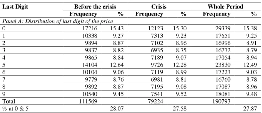
Table no. 2 shows the frequency with which the last digits of closing prices are observed in the US sample, the results of the clustering tests and also the values of HHI.
Table no. 2 – Price clustering in the US banks’ subsample
Last Digit Before the crisis Crisis Whole Period
Frequency % Frequency % Frequency %
Panel A: Distribution of last digit of the price
0 17216 15.43 12123 15.30 29339 15.38 1 10338 9.27 7313 9.23 17651 9.25 2 9894 8.87 7102 8.96 16996 8.91 3 9837 8.82 6935 8.75 16772 8.79 4 9865 8.84 7189 9.07 17054 8.94 5 14104 12.64 9726 12.28 23830 12.49 6 10104 9.06 7119 8.99 17223 9.03 7 9779 8.76 6981 8.81 16760 8.78 8 9892 8.87 7195 9.08 17087 8.96 9 10540 9.45 7541 9.52 18081 9.48 Total 111569 79224 190793 % at 0 & 5 28.07 27.58 27.87
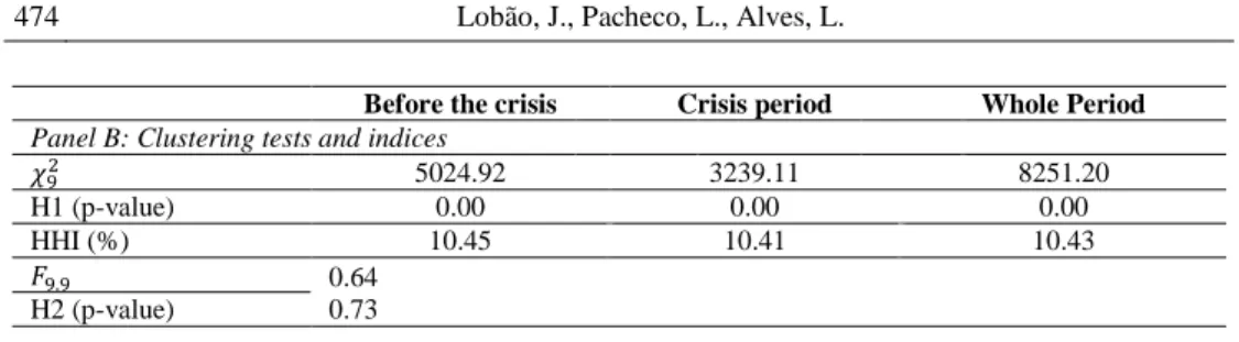
Before the crisis Crisis period Whole Period Panel B: Clustering tests and indices
𝜒92 5024.92 3239.11 8251.20 H1 (p-value) 0.00 0.00 0.00 HHI (%) 10.45 10.41 10.43 𝐹9.9 0.64 0.73 H2 (p-value)
Note: Panel A shows the absolute and the relative frequencies of prices. Panel B presents the p-value of the H1 and H2 hypotheses, as well as the HHI, which stands for the Hirschman-Herfindahl index.
Table no. 3 – Clustering of the final digit of price for various partitions of the US sample Percentage of cases clustered at a final digit of
Quintiles 0 1 2 3 4 5 6 7 8 9 HHI (%) All prices 14.52 9.40 9.06 8.99 9.07 11.99 9.16 9.01 9.10 9.69 10.30 Size 1 18.49 8.91 8.14 8.10 8.32 13.94 8.61 8.05 8.29 9.16 11.08 2 15.04 9.16 8.92 8.66 9.04 12.16 9.22 8.91 8.89 10.00 10.38 3 13.62 9.62 9.34 9.27 9.50 11.36 9.29 9.26 9.21 9.53 10.18 4 12.79 9.64 9.58 9.35 9.33 11.17 9.39 9.45 9.51 9.78 10.11 5 12.70 9.69 9.33 9.57 9.14 11.30 9.31 9.39 9.62 9.95 10.11 Price 1 15.46 9.22 9.21 8.59 8.94 12.65 8.97 8.55 9.01 9.40 10.46 2 14.95 9.18 8.78 8.93 9.03 12.23 9.21 8.85 8.95 9.91 10.37 3 14.62 9.42 9.19 8.63 9.14 11.82 9.23 9.06 8.98 9.91 10.31 4 14.05 9.54 9.02 9.35 9.07 11.61 9.41 9.13 9.14 9.67 10.23 5 13.54 9.64 9.13 9.44 9.16 11.63 9.00 9.47 9.43 9.54 10.19 Volatility 1 14.47 9.28 9.41 9.10 9.13 12.10 8.84 8.86 9.12 9.67 10.30 2 14.40 9.48 9.05 8.95 9.12 11.92 9.07 8.82 9.19 10.00 10.29 3 14.03 9.43 9.26 9.12 9.24 11.76 9.26 9.22 9.21 9.46 10.24 4 15.15 9.23 8.69 8.95 8.74 12.36 9.33 9.01 8.94 9.60 10.40 5 14.58 9.59 8.90 8.82 9.11 11.79 9.32 9.14 9.06 9.70 10.30 Turnover 1 17.93 9.06 8.30 8.19 8.37 13.68 8.69 8.18 8.29 9.30 10.95 2 15.45 9.10 8.97 8.63 9.01 12.17 9.24 8.86 8.90 9.65 10.42 3 13.89 9.55 9.19 9.13 9.33 11.80 9.13 9.12 9.14 9.72 10.23 4 12.96 9.53 9.40 9.34 9.34 11.25 9.33 9.56 9.45 9.84 10.13 5 12.40 9.77 9.46 9.65 9.28 11.04 9.43 9.33 9.72 9.91 10.09 Illiquidity 1 12.40 9.81 9.42 9.41 9.50 10.85 9.45 9.62 9.56 9.98 10.08 2 12.91 9.70 9.57 9.47 9.12 11.40 9.01 9.29 9.62 9.91 10.13 3 14.15 9.34 9.15 9.23 9.30 11.45 9.41 9.11 9.04 9.81 10.24 4 14.33 9.20 9.10 8.97 9.12 12.18 9.37 9.12 9.09 9.52 10.29 5 18.85 8.96 8.07 7.86 8.29 14.07 8.57 7.92 8.21 9.20 11.17
Note: the table shows the clustering of the final digit of price for various partitions of the US sample during the whole period, including the pre-crisis and the crisis period. Only the stocks with data available for all variables were included. The measure of clustering HHI stands for the Herfindahl-Hirschman Index.
There is clear evidence of price clustering for both periods, with almost 30% of prices having as last digits 0 or 5. Panel B confirms the existence of a statistically significant
clustering for the period before the crisis and for the crisis period. The H1 null hypothesis of absence of clustering is clearly rejected for both periods for a significance level of 1%. HHI values decrease slightly from the pre-crisis period to the crisis period, but this difference is not statistically significant. The nonexistence of a higher level of clustering in the crisis period goes counter what is predicted by the Panic Trading hypothesis (Narayan and Smyth, 2013).
Table no. 3 shows a more detailed analysis of price clustering as a function of some variables representative of company-specific attributes.
For each one of the attributes (size, price level, volatility, turnover and illiquidity), we sort the stocks into quintiles from low to high. According to the Price Resolution/Negotiation hypotheses, one would expect a higher level of clustering for smaller and more volatile banks, for higher price levels, for less traded shares and for higher levels of illiquidity.
The results of this analysis partially confirm the predictions of the Price Resolution/Negotiation hypotheses. In fact, it is noticeable that the factors size and turnover seem to be negatively related to clustering and that there is a higher price concentration for higher levels of illiquidity. The results for the price and volatility variables are inconclusive. Table no. 4 shows the results regarding the sample of European banks. The evidence is analogous to that obtained with the US sample.
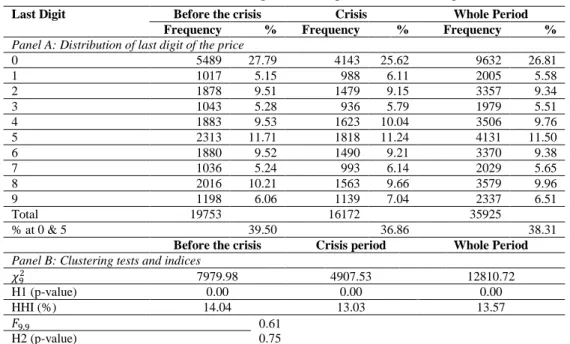
Table no. 4 – Price clustering in the European banks’ subsample
Last Digit Before the crisis Crisis Whole Period
Frequency % Frequency % Frequency %
Panel A: Distribution of last digit of the price
0 5489 27.79 4143 25.62 9632 26.81 1 1017 5.15 988 6.11 2005 5.58 2 1878 9.51 1479 9.15 3357 9.34 3 1043 5.28 936 5.79 1979 5.51 4 1883 9.53 1623 10.04 3506 9.76 5 2313 11.71 1818 11.24 4131 11.50 6 1880 9.52 1490 9.21 3370 9.38 7 1036 5.24 993 6.14 2029 5.65 8 2016 10.21 1563 9.66 3579 9.96 9 1198 6.06 1139 7.04 2337 6.51 Total 19753 16172 35925 % at 0 & 5 39.50 36.86 38.31
Before the crisis Crisis period Whole Period Panel B: Clustering tests and indices
𝜒92 7979.98 4907.53 12810.72 H1 (p-value) 0.00 0.00 0.00 HHI (%) 14.04 13.03 13.57 𝐹9.9 0.61 0.75 H2 (p-value)
Note: Panel A shows the absolute and the relative frequencies of prices. Panel B presents the p-value of the H1 and H2 hypotheses, as well as the HHI, which stands for the Hirschman-Herfindahl index.
Again, there is an abnormal concentration in prices, even more pronounced than in the sample of US banks. The percentage of prices whose last digit is 0 or 5 is around 40% and 37% for the period before the crisis and for the crisis period, respectively. The results also indicate a clear rejection of the null hypothesis H1 and, consequently, the presence of
statistically significant price clustering in both periods. HHI is slightly higher in the period before the crisis, but the results of the H2 hypothesis test, as happened in the US sample, do not allow the rejection of the null hypothesis of similar clustering levels in the two periods. Table no. 5 presents a detailed analysis of clustering of the final digit of price for various partitions of the European sample.
Table no. 5 – Clustering of the final digit of price for various partitions of the European sample Percentage of cases clustered at a final digit of
Quintiles 0 1 2 3 4 5 6 7 8 9 HHI (%) All prices 24.97 5.68 9.82 5.67 10.39 10.56 9.88 5.86 10.58 6.60 12.91 Size 1 19.04 4.72 11.97 5.41 12.77 7.97 12.19 6.33 12.58 7.02 11.80 2 23.91 6.45 8.65 6.73 10.13 12.87 8.71 5.86 9.31 7.37 12.53 3 24.61 5.96 9.75 5.57 10.12 11.66 9.59 5.93 10.37 6.45 12.82 4 28.71 4.75 10.41 4.33 10.83 7.38 11.31 5.13 11.91 5.26 14.69 5 28.53 6.53 8.34 6.29 8.10 12.88 7.60 6.08 8.75 6.91 14.16 Price 1 21.55 4.39 11.86 4.44 14.55 8.04 12.59 4.49 12.81 5.30 12.91 2 15.25 7.24 10.88 8.18 10.10 10.33 10.47 8.34 10.72 8.49 10.45 3 31.10 4.40 9.86 4.28 10.08 8.26 10.56 4.57 11.87 4.99 15.71 4 22.67 7.03 9.43 6.53 9.76 11.95 9.31 6.98 9.00 7.33 12.03 5 34.31 5.33 7.07 4.88 7.45 14.19 6.45 4.93 8.52 6.87 17.22 Volatility 1 20.98 6.45 9.40 7.10 9.80 10.44 9.46 7.80 10.14 8.44 11.50 2 18.90 7.52 9.47 7.83 10.29 11.39 9.57 7.35 9.97 7.71 11.05 3 29.71 2.21 14.03 1.83 15.28 3.15 14.59 2.13 14.81 2.27 17.73 4 26.30 4.94 9.94 5.47 10.04 10.93 9.20 5.67 11.15 6.37 13.47 5 28.99 7.25 6.31 6.06 6.57 16.81 6.62 6.34 6.88 8.18 14.93 Turnover 1 30.81 3.34 11.80 3.06 11.85 6.73 12.11 3.12 13.25 3.92 16.42 2 26.66 5.33 9.49 5.61 9.82 9.96 9.60 5.92 11.03 6.60 13.49 3 23.20 4.74 10.78 5.28 12.65 9.66 11.06 5.00 11.50 6.11 12.76 4 26.38 6.61 8.34 5.55 9.12 12.73 8.23 6.58 8.40 8.06 13.32 5 17.85 8.35 8.71 8.78 8.52 13.68 8.40 8.66 8.75 8.29 10.92 Illiquidity 1 17.82 8.23 8.97 8.50 8.83 13.29 8.18 8.66 8.72 8.81 10.88 2 21.61 7.22 7.98 7.64 8.15 14.54 7.88 8.07 8.19 8.73 11.89 3 28.76 6.37 8.12 6.03 8.10 12.58 7.63 5.83 9.30 7.28 14.26 4 25.74 5.52 8.91 5.33 9.94 10.91 10.19 5.86 10.32 7.28 13.16 5 31.03 0.99 15.22 0.66 17.06 1.26 15.63 0.82 16.49 0.82 20.06
Note: The table shows the clustering of the final digit of price for various partitions of the European sample during the whole period, including the pre-crisis and the crisis period. Only the stocks with data available for all variables were included. HHI, the measure of clustering, stands for the Herfindahl-Hirschman Index. The results suggest a positive relationship between bank size and the level of clustering. As for the other specific attributes, the results confirm the Price Resolution/ Negotiation hypotheses with respect to turnover and illiquidity. This analysis also seems to suggest larger levels of clustering for stocks with higher prices, whereas the results are inconclusive regarding volatility.
In sum, the results point to the presence of clustering in all periods of both samples. The digits 0 and 5 are invariably the most frequently observed. The level of clustering seems to be higher in the sample of European banks. Surprisingly, we did not find any statistically significant differences between the pre-crisis and the crisis clustering levels, either for the sample of European banks or for the sample of US banks. Our univariate analysis partially confirmed the predictions of the Price Resolution/Negotiation hypotheses, as well as the Attraction hypothesis.
4.2 Multivariate analysis
4.2.1 US banks
For each sample and for each period two models were estimated, one with all the explanatory variables (I) and other where one variable whose correlation coefficient with other factors is high (greater than 0.6) was excluded in order to avoid problems of multicollinearity (II). Table no. 6 presents the results for the US sample.
According to the Price Resolution/Negotiation hypotheses, the variables "Price", "RetVol" and "Illiquidity" should have a positive relationship with clustering, while the variables "Size" and "Turnover" should be negatively associated with the phenomenon. On one hand, our results show that the relation predicted by the theory for the variables "Turnover" and "Illiquidity" is confirmed at a statistically significant level of 1% for the "Illiquidity" variable in both periods, with the "Turnover" variable being also statistically significant at a level of 1% in the period before the crisis. On the other hand, the expected results for the variables "Size" and "RetVol" are not confirmed. Moreover, the variable "Price" is not statistically significant. On an overall assessment, we can conclude that the Price Resolution/Negotiation hypotheses are only partially confirmed in our sample of US banks.
“Size” is statistically significant at a significance level of 10% for both periods in the model with all the explanatory variables. However this variable only has significant explanatory power for the crisis period in the reduced model. As we have mentioned above the results show a relationship between this variable and the dependent variable that is surprising according to the Price Resolution hypothesis. However, the variable "SizeAssetsBV", which captures the banks' risk has coefficients with a negative sign for both periods, corresponding to what is predicted by the Price Resolution/Negotiation hypotheses. In the second model, the “Size” variable continues to show a coefficient with a positive sign in the crisis period which runs counter to what was expected.
The "PastReturns" variable is not statistically significant for any of the periods under analysis. The variable "BTM" variable is statistically significant only for the period before the crisis, having negative regression coefficients. This suggests that growth stocks are more affected by clustering in the period before the crisis. The "AnalystCoverage" variable is not statistically significant in all estimated models for significance levels of 10%.
The variables that measure the banks’ opacity present dissimilar results. The variables “Loans” and “Investments” are only statistically significant at the conventional levels in the crisis period, while the variable “Deposits” has no statistical significance in any of the periods.
Table no. 6 – Determinants of price clustering (US sample)
Note: standard errors in parenthesis; ***, ** and * represent statistical significance at the 1%, 5% and 10% levels, respectively.
The variables “SizeAssetsBV”, "TobinQ" and “CreditRisk that measure the banks’ risks are only statistically significant for the periods before the crisis. The sign of the coefficient of "TobinQ" in this period is negative, which is in accordance with the theory. As for the variables “SizeAssetsBV” and "CreditRisk", they present a negative coefficient,
Before the crisis Crisis period
Variable (I) (II) (I) (II) Expected sign
α 0.0066*** (0.0005) 0.0066*** (0.0005) 0.0061*** (0.0003) 0.0061*** (0.0003) Size 0.0128** (0.0050) 0.0007 (0.0012) 0.0035* (0.0019) 0.0021*** (0.0008) - Price -0.0004 (0.0006) -0.0004 (0.0006) -0.0006 (0.0005) -0.0006 (0.0005) + RetVol -0.0012** (0.0006) -0.0013** (0.0006) -0.0019*** (0.0005) -0.0021*** (0.0005) + Turnover -0.0027*** (0.0010) -0.0018* (0.0010) -0.0012 (0.0008) -0.0011 (0.0008) - Illiquidity 0.0041*** (0.0007) 0.0046*** (0.0007) 0.0044*** (0.0005) 0.0044*** (0.0005) + PastReturns -0.0005 (0.0006) -0.0001 (0.0006) -0.0005 (0.0004) -0.0005 (0.0004) - BTM -0.0027** (0.0013) -0.0012 (0.0011) 0.0000 (0.0007) -0.0001 (0.0007) - AnalystCoverage 0.0010 (0.0008) 0.0004 (0.0008) -0.0005 (0.0004) -0.0005 (0.0004) - Loans -0.0005 (0.0010) -0.0012 (0.0009) -0.0011* (0.0007) -0.0012* (0.0007) + Investments -0.0010 (0.0008) -0.0016* (0.0008) -0.0013** (0.0006) -0.0015** (0.0006) + Deposits 0.0000 (0.0009) 0.0006 (0.0008) 0.0002 (0.0006) 0.0003 (0.0006) + SizeAssetsBV -0.0123** (0.0050) -0.0015 (0.0018) + TobinQ -0.0044** (0.0018) -0.0009 (0.0011) -0.0009 (0.0007) -0.0007 (0.0006) - CreditRisk -0.0011** (0.0005) -0.0010* (0.0005) -0.0002 (0.0005) -0.0002 (0.0005) + ROAVOL 0.0019 (0.0101) 0.0104 (0.0097) -0.0024 (0.0089) -0.0017 (0.0089) + NIMVOL -0.0003 (0.0005) -0.0002 (0.0005) 0.0000 (0.0003) 0.0000 (0.0003) + ZSCORE 0.0018 (0.0102) 0.0100 (0.0098) -0.0024 (0.0089) -0.0017 (0.0089) - R-squared 0.4334 0.4132 0.5625 0.5608 Adjusted R-squared 0.3774 0.3589 0.5192 0.5201 F-statistic 7.7385 7.6133 13.0066 13.8037 Prob(F-statistic) 0.0000 0.0000 0.0000 0.0000
contrary to what was expected. The remaining variables, "ROAVOL", "NIMVOL" and "ZSCORE" are not statistically significant at the conventional levels.
The variables that best appear to explain clustering are “Size”, “RetVol”, and “Illiquidity”. “Size” and “Illiquidity” positively affect the level of clustering and the volatility of returns has a negative impact on it. Only the relationship between “Illiquidity” and the dependent variable is consistent with what is predicted by the Price Resolution/ Negotiation hypotheses.
4.2.2 European banks
Table no. 7 presents the regressions’ results for the sample of European banks.
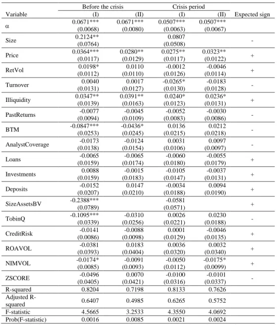
The evidence regarding the model that includes all explanatory variables (model I) indicates that the relation predicted by the Price Resolution/Negotiation hypotheses for the variables “Price”, “RetVol”, "Turnover" and "Illiquidity" is confirmed at the conventional levels of statistical significance, although some of these variables are only significant for one of the periods under scrutiny. The variable “RetVol” presents some explanatory power in the period before the crisis, but it does not explain price clustering in the crisis period. “Turnover”, in turn, only has some explanatory power in the crisis period. The expected results for the variable "Size" are not confirmed. This variable seems to explain the price clustering phenomenon better in the period before the crisis than in the crisis period. Statistically, the difference between the coefficients from one period to the other is not significant. Because they showed high correlation coefficients with other variables, “Size” and “SizeAssetsBV” were eliminated from the most complete model and a new regression without these variables was estimated for each of the periods (model II), without greatly affecting the results.
Overall, we can conclude that the Price Resolution/Negotiation hypotheses are only partially confirmed in our sample of European banks.
"PastReturns" and "AnalystCoverage" do not contribute to explain the price clustering. The "BTM" variable is statistically significant for the period before the crisis and it has a negative coefficient. The variables "Loans", “Investments" and "Deposits" have no significant explanatory power. Thus, the opacity factor does not seem to be relevant for the price clustering in European banks.
Regarding the risk measures, the variable "SizeAssetsBV" is statistically significant for the period before the crisis, presenting a negative coefficient. This is in accordance with the Price Resolution theory. “TobinQ”, another measure of risk, only explains the clustering in the pre-crisis period. The negative coefficient is consistent with the prediction that a higher risk tends to generate stronger price clustering. "CreditRisk", "ROAVOL" and "ZSCORE" are not statistically significant for any of the periods and "NIMVOL" is statistically significant only for the pre-crisis period. However, the negative coefficient runs counter to what is predicted by the theory. These results suggest that risk only seems to explain clustering in Europe in the period leading to the Global Financial Crisis.
Table no. 7 – Determinants of price clustering (European sample)
Note: standard errors in parenthesis; ***, ** and * represent statistical significance at the 1%, 5% and 10% levels, respectively.
In sum, “Price” and “Illiquidity” are the variables that best seem to explain the variation in clustering in European banks. There are some factors (for example, “Size”, “RetVol”, “BTM”) that contribute to explain this variation in only one of the periods.
Before the crisis Crisis period
Variable (I) (II) (I) (II) Expected sign
0.0671*** (0.0068) 0.0671*** (0.0080) 0.0507*** (0.0063) 0.0507*** (0.0067) Size 0.2124** (0.0764) 0.0807 (0.0508) - Price 0.0364*** (0.0117) 0.0280** (0.0129) 0.0275** (0.0117) 0.0323** (0.0122) + RetVol 0.0198* (0.0112) 0.0110 (0.0110) -0.0012 (0.0126) -0.0046 (0.0114) + Turnover 0.0040 (0.0131) 0.0017 (0.0127) -0.0265* (0.0130) -0.0183 (0.0128) - Illiquidity 0.0347** (0.0139) 0.0391** (0.0163) 0.0240* (0.0123) 0.0236* (0.0131) + PastReturns -0.0077 (0.0094) -0.0045 (0.0109) -0.0052 (0.0083) -0.0030 (0.0086) - BTM -0.0847*** (0.0253) -0.0436* (0.0245) 0.0136 (0.0215) 0.0212 (0.0218) - AnalystCoverage -0.0173 (0.0138) -0.0124 (0.0154) 0.0031 (0.0106) 0.0097 (0.0097) - Loans -0.0065 (0.0159) -0.0065 (0.0174) -0.0060 (0.0180) -0.0055 (0.0179) + Investments 0.0088 (0.0159) -0.0015 (0.0183) -0.0105 (0.0147) -0.0037 (0.0131) + Deposits -0.0152 (0.0207) 0.0147 (0.0210) -0.0034 (0.0188) 0.0094 (0.0190) + SizeAssetsBV -0.2388*** (0.0789) -0.0581 (0.0571) + TobinQ -0.1095*** (0.0339) -0.0310 (0.0256) 0.0026 (0.0221) 0.0230 (0.0188) - CreditRisk -0.0141 (0.0086) -0.0088 (0.0098) 0.0001 (0.0129) -0.0046 (0.0135) + ROAVOL -0.0381 (0.0393) 0.0183 (0.0404) 0.0036 (0.0320) 0.0032 (0.0340) + NIMVOL -0.0174* (0.0085) -0.0091 (0.0093) -0.0050 (0.0112) -0.0175* (0.0099) + ZSCORE -0.0496 (0.0405) 0.0070 (0.0421) -0.0100 (0.0316) -0.0101 (0.0337) - R-squared 0.8204 0.7198 0.8133 0.7626 Adjusted R-squared 0.6407 0.4985 0.6265 0.5752 F-statistic 4.5665 3.2533 4.3550 4.0692 Prob(F-statistic) 0.0016 0.0085 0.0021 0.0024
4.2.3 Comparing US banks with European banks
Our results partially confirm the Price Resolution/Negotiation hypotheses. In both samples, the variables “Turnover” and “Illiquidity” have a relation with price clustering as predicted by the theory, although “Turnover” is only statistically significant in the crisis period in the European sample. “Illiquidity” is the only explanatory variable that helps to explain the price clustering for both geographical areas and for both periods. The results for “Price” and “RetVol” in the European banks’ sample also support the Price Resolution/Negotiation hypotheses, while “Size” has a relation with clustering in both samples that goes against what was expected.
The "BTM" variable is statistically significant only for the periods before the crisis in both samples. The negative coefficient is in accordance with the theory.
“Loans” and “Investments” capture banks’ opacity and present explanatory power during the crisis period in the US. However, the relationship with clustering is not in accordance to what was expected. In the European sample, all opacity variables are not statistically significant. Regarding the risk measures, “SizeAssetsBV” and “TobinQ” have some explanatory power but only in the pre-crisis period. “Credit Risk” is also relevant to explain clustering in this period but only in the US. The results for the variable “TobinQ” also support the theory. We can conclude from these results that opacity and risk do not contribute significantly to the degree of clustering at the firm level.
There are variables that do not contribute to this explanation in any of the periods and geographic areas under analysis: “PastReturns”, “AnalystCoverage”, “Deposits”, “ROAVOL” and “ZSCORE”.
It is also worth noting that the coefficients of a large part of the variables between the two periods under analysis do not differ significantly. In the US sample, for example, only “Size” exhibits a decrease in the positive impact on the clustering level from the pre-crisis period to the crisis period. This suggests that the Global Financial Crisis did not play a significant role in the phenomenon of price clustering in bank stocks.
4.3 Impact of the European sovereign debt crisis
In addition to the analyses that we have already presented, it seemed appropriate to extend this study to the sovereign debt crisis that occurred in Europe.
The sovereign debt crisis had a substantial economic and political impact on Greece, Italy, Portugal and Spain. The purpose of this analysis is to separate the sample of European banks into two subsamples: one with the banks of countries affected by the crisis and another with the other banks of European countries where the crisis has not had a significant impact.
We conduct a similar analysis to that implemented in the univariate analysis, based on the comparison between the price clustering levels between the two subsamples of European banks. The period of analysis considered runs between September 1, 2008 and August 4, 2011, following the crisis period defined by Beirne and Fratzscher (2013). Table no. 8 presents the results.
Table no. 8 – Impact of the European sovereign debt crisis on price clustering Last Digit Affected countries Non-affected countries
Frequency % Frequency %
Panel A: Distribution of last digit of the price
0 2727 16.39 2333 26.80 1 1401 8.42 671 7.71 2 1585 9.53 599 6.88 3 1346 8.09 588 6.75 4 1529 9.19 537 6.17 5 2099 12.62 1463 16.80 6 1496 8.99 587 6.74 7 1339 8.05 497 5.71 8 1640 9.86 682 7.83 9 1476 8.87 749 8.60 Total 16638 8706 % at 0 & 5 29.01 43.60
Affected countries Non-affected countries
Panel B: Clustering tests and indices
𝜒92 1011.97 3520.18
H1 (p-value) 0.0000 0.0000
HHI (%) 10.61 14.04
𝐹9.9 3.48
H2 (p-value) 0.0387
Note: Panel A shows the absolute and the relative frequencies of prices. Panel B presents the p-value of the H1 and H2 hypotheses, as well as the HHI, which stands for the Hirschman-Herfindahl index. The sample of European banks was divided into two subsamples: a sample with the banks of countries affected by the European sovereign debt crisis (Greece, Italy, Portugal and Spain) and other with the banks of European countries where the crisis has not had such a significant impact (Austria, Denmark, Finland, Germany, Romania).
We can conclude that there are signs of an abnormal concentration of prices for both samples, as suggested by the p-values of the H1 hypothesis. Once again, digits 0 and 5 are the most frequently observed, reaching a percentage of more than 40% in the sample of non-affected countries, more than twice what would be expected if the price distribution was uniform. Analyzing the results of Panel B, we can also see that the HHI for the sample of countries where the sovereign debt crisis has not been felt so strongly is significantly higher than for the sample of countries affected by the crisis. The clustering observed in the stock prices of the banks of unaffected countries is, at a level of statistical significance of 5%, higher than that observed in the sample of the countries that had problems with their public debt.
The evidence of a lower level of clustering at times of crisis is quite surprising, being however in line the previously presented results. The implications of this result are further discussed in the conclusion.
5. CONCLUSION
This paper examines the impact of the Global Financial Crisis on price clustering in US and European banking stocks.
Our evidence confirms the existence of significant price clustering in both geographies. Investors exhibit a clear preference for prices with a final digit of 0 and 5 which is consistent with the Attraction hypothesis. The existence of a pervasive pattern of accumulation of
prices in certain digits is difficult to reconcile with the Efficient Market hypothesis since one of the tenets of an efficient market is that prices should follow a random walk. The empirical finding that clustering leads to desestabilized stock prices seems to underline the apparent conflict between the phenomenon and stock market efficiency (Blau and Griffith, 2016). The observation that prices tend to be settled more frequently at some numbers than others also carry practical implications for traders. It has been shown that investors can devise profitable trading strategies to exploit clustering effects even after considering the bid-ask spread (Niederhoffer, 1965; Mitchell, 2001). Examples of such strategies are provided in Niederhoffer (1965).
We conduct one of the first tests to the recently proposed Panic Trading hypothesis (Narayan and Smyth, 2013) by examining the difference between the levels of price clustering observed before the crisis and in the crisis period. Our results do not reveal a significant increase in the levels of price clustering in the crisis period which is at odds with the Panic Trading hypothesis. In fact, the crisis period witnessed a lower level of price clustering.
We also performed a multivariate analysis of price clustering in order to understand the firm-specific factors that produce price clustering effects. In both samples, the variables “Turnover” and “Illiquidity” present a statistical significant relation with price clustering. These results are consistent with the Price Resolution/Negotiation hypotheses.
The evidence of a lower level of clustering at times of crisis is quite surprising. This relationship between the level of clustering and periods of crisis suggests that investors are less affected by behavioral factors in periods of greater pessimism. This finding is consistent with some contributions in the literature. For example, the mood-as-information hypothesis argues that mood affects human decisions and that, as argued by Schwarz (1990, p. 527), "negative affective states, which inform the organism that its current situation is problematic, foster the use of effortful, detail-oriented, analytical processing, whereas positive affective states foster the use of less effortful heuristic strategies". Moreover, Alloy and Abramson (1979) conclude that individuals, at depressive times, tend to be more realistic and more analytical in their appraisals (the "sadder but wiser" effect). Isen (1987), Sinclair and Mark (1995) and Durand et al. (2009) suggest that individuals make more logical, consistent and unbiased decisions when they find themselves in a negative affective state, a consequence of an instinct to turn a bad situation into a good one.
In addition to these studies, some Behavioral Finance papers suggest that investors are better at processing information at times when the market sentiment is negative. For example, Cooper et al. (2004) find that the profits to momentum strategies depend critically on the state of the market. Investors seem to interpret the information in a more efficient fashion in periods of negative mood. García (2013) corroborates this reasoning showing that prices reflect much more quickly the news published in the financial section of The New
York Times during periods of recession. Thus, at the origin of this relationship between the
periods of crisis and the level of price clustering might be a greater rationality and analytical capacity of investors in periods of negative sentiment.
Finally, as suggestions for further research, it would be interesting to ascertain the impact of other crises on price clustering. In addition, it would also be of interest to understand the impact of market trends on the phenomenon.
ORCID
Júlio Lobão https://orcid.org/0000-0001-5896-9648 Luís Pacheco https://orcid.org/0000-0002-9066-6441
References
Aitken, M., Brown, P., Buckland, C., Izan, H. Y., and Walter, T., 1996. Price clustering on the Australian Stock Exchange. Pacific-Basin Finance Journal, 4(2-3), 297-314. http://dx.doi.org/10.1016/0927-538X(96)00016-9
Alloy, L. B., and Abramson, L. Y., 1979. Judgment of contingency in depressed and nondepressed students: Sadder but wiser? Journal of Experimental Psychology. General, 108(4), 441-485. http://dx.doi.org/10.1037/0096-3445.108.4.441
Anderson, R. C., and Fraser, D. R., 2000. Corporate control, bank risk taking, and the health of the banking industry. Journal of Banking & Finance, 24(8), 1383-1398. http://dx.doi.org/10.1016/S0378-4266(99)00088-6
ap Gwilym, O., Clare, A., and Thomas, S., 1998. Extreme price clustering in the London equity index futures and options markets. Journal of Banking & Finance, 22(9), 1193-1206. http://dx.doi.org/10.1016/S0378-4266(98)00054-5
Aşçıoğlu, A., Comerton-Forde, C., and McInish, T. H., 2007. Price clustering on the Tokyo stock exchange. Financial Review, 42(2), 289-301. http://dx.doi.org/10.1111/j.1540-6288.2007.00172.x
Athanasoglou, P. P., Brissimis, S. N., and Delis, M. D., 2008. Bank-specific, industry-specific and macroeconomic determinants of bank profitability. Journal of International Financial Markets,
Institutions and Money, 18(2), 121-136. http://dx.doi.org/10.1016/j.intfin.2006.07.001
Attinasi, M. G., Checherita-Westphal, C. D., and Nickel, C., 2009. What explains the surge in euro area sovereign spreads during the financial crisis of 2007-09? . European Central Bank Working
Paper(1131).
Baig, A., Blau, B. M., and Sabah, N., 2019. Price clustering and sentiment in bitcoin. Finance
Research Letters, 29, 111-116. http://dx.doi.org/10.1016/j.frl.2019.03.013
Ball, C. A., Torous, W. N., and Tschoegl, A. E., 1985. The degree of price resolution: The case of the gold market. Journal of Futures Markets, 5(1), 29-43. http://dx.doi.org/10.1002/fut.3990050105 Beirne, J., and Fratzscher, M., 2013. The pricing of sovereign risk and contagion during the European
sovereign debt crisis. Journal of International Money and Finance, 34, 60-82. http://dx.doi.org/10.1016/j.jimonfin.2012.11.004
Berger, A. N., Bonime, S. D., Covitz, D. M., and Hancock, D., 2000. Why are bank profits so persistent? The roles of product market competition, informational opacity, and regional/macroeconomic shocks. Journal of Banking & Finance, 24(7), 1203-1235. http://dx.doi.org/10.1016/S0378-4266(99)00124-7
Bharati, R., Crain, S. J., and Kaminski, V., 2012. Clustering in crude oil prices and the target pricing
zone hypothesis. Energy Economics, 34(4), 1115-1123.
http://dx.doi.org/10.1016/j.eneco.2011.09.009
Blau, B. M., and Griffith, T. G., 2016. Price clustering and the stability of stock prices. Journal of
Business Research, 69(10), 3933-3942. http://dx.doi.org/10.1016/j.jbusres.2016.06.008
Brown, A., and Yang, F., 2016. Limited cognition and clustered asset prices: Evidence from betting
markets. Journal of Financial Markets, 29, 27-46.
http://dx.doi.org/10.1016/j.finmar.2015.10.003
Brown, P., Chua, A., and Mitchell, J., 2002. The influence of cultural factors on price clustering: Evidence from Asia-Pacific stock markets. Pacific-Basin Finance Journal, 10(3), 307-332. http://dx.doi.org/10.1016/S0927-538X(02)00049-5
Brown, P., and Mitchell, J., 2008. Culture and stock price clustering: Evidence from The Peoples' Republic of China. Pacific-Basin Finance Journal, 16(1), 95-120. http://dx.doi.org/10.1016/j.pacfin.2007.04.005
Christie, W. G., Harris, J. H., and Schultz, P. H., 1994. Why did NASDAQ market makers stop avoiding odd-eighth quotes? The Journal of Finance, 49(5), 1841-1860. http://dx.doi.org/10.1111/j.1540-6261.1994.tb04783.x
Cooper, M. J., Gutierrez, R. C., and Hameed, A., 2004. Market states and momentum. The Journal of
Finance, 59(3), 1345-1365. http://dx.doi.org/10.1111/j.1540-6261.2004.00665.x
Curcio, R., and Goodhart, C., 1991. The clustering of bid/ask prices and the spread in the foreign
exchange market: LSE Financial Markets Group.
Das, S., and Kadapakkam, P. R., 2018. Machine over mind? Stock price clustering in the era of algorithmic trading. The North American Journal of Economics and Finance, 100831. http://dx.doi.org/10.1016/j.najef.2018.08.014
Davis, S., Madura, J., and Marciniak, M., 2009. Performance and risk among types of Exchange-Traded Funds during the financial crisis. ETFs and Indexing(1), 182-188.
De Grauwe, P., and Decupere, D., 1992. Psychological barriers in the foreign exchange market. CEPR
Discussion Papers, 621.
Durand, R. B., Simon, M., and Szimayer, A., 2009. Anger, sadness and bear markets. Applied
Financial Economics, 19(5), 357-369. http://dx.doi.org/10.1080/09603100801964362
García, D., 2013. Sentiment during recessions. The Journal of Finance, 68(3), 1267-1300. http://dx.doi.org/10.1111/jofi.12027
Hameed, A., and Terry, E., 1998. The effect of tick size on price clustering and trading volume.
Journal of Business Finance & Accounting, 25(7-8), 849-867. http://dx.doi.org/10.1111/1468-5957.00216
Harris, L., 1991. Stock-price clustering and discreteness. Review of Financial Studies, 4(3), 389-415. http://dx.doi.org/10.1093/rfs/4.3.389
Hu, B., Jiang, C., McInish, T., and Ning, Y., 2019. Price Clustering of Chinese IPOs: The Impact of Regulation, Cultural Factors, and Negotiation. Applied Economics, 51(36), 3995-4007. http://dx.doi.org/10.1080/00036846.2019.1588946
Huang, R. D., and Stoll, H. R., 1996. Dealer versus auction markets: A paired comparison of execution costs on NASDAQ and the NYSE. Journal of Financial Economics, 41(3), 313-357. http://dx.doi.org/10.1016/0304-405X(95)00867-E
Ikenberry, D. L., and Weston, J. P., 2008. Clustering in US stock prices after decimalisation. European
Financial Management, 14(1), 30-54. http://dx.doi.org/10.1111/j.1468-036X.2007.00410.x Isen, A. M., 1987. Positive affect, cognitive processes, and social behavior (pp. 203-253): Academic
Press. http://dx.doi.org/10.1016/S0065-2601(08)60415-3
Kanagaretnam, K., Lim, C. Y., and Lobo, G. J., 2014. Influence of national culture on accounting conservatism and risk-taking in the banking industry. The Accounting Review, 89(3), 1115-1149. http://dx.doi.org/10.2308/accr-50682
Kandel, S., Sarig, O., and Wohl, A., 2001. Do investors prefer round stock prices? Evidence from Israeli IPO auctions. Journal of Banking & Finance, 25(8), 1543-1551. http://dx.doi.org/10.1016/S0378-4266(00)00131-X
Laeven, L., and Levine, R., 2009. Bank governance, regulation and risk taking. Journal of Financial
Economics, 93(2), 259-275. http://dx.doi.org/10.1016/j.jfineco.2008.09.003
Lakonishok, J., Shleifer, A., and Vishny, R. W., 1994. Contrarian investment, extrapolation, and risk.
The Journal of Finance, 49(5), 1541-1578. http://dx.doi.org/10.1111/j.1540-6261.1994.tb04772.x
Lee, C., and Swaminathan, B., 2000. Price momentum and trading volume. The Journal of Finance,
55(5), 2017-2069. http://dx.doi.org/10.1111/0022-1082.00280
Mitchell, J., 2001. Clustering and psychological barriers: The importance of numbers. Journal of