EUROPEAN ORGANIZATION FOR NUCLEAR RESEARCH (CERN)
CERN-PH-EP/2012-262 2013/05/30
CMS-BTV-12-001
Identification of b-quark jets with the CMS experiment
The CMS Collaboration
∗Abstract
At the Large Hadron Collider, the identification of jets originating from b quarks is important for searches for new physics and for measurements of standard model processes. A variety of algorithms has been developed by CMS to select b-quark jets based on variables such as the impact parameters of charged-particle tracks, the properties of reconstructed decay vertices, and the presence or absence of a lepton, or combinations thereof. The performance of these algorithms has been measured using data from proton-proton collisions at the LHC and compared with expectations based on simulation. The data used in this study were recorded in 2011 at√s =7 TeV for a total integrated luminosity of 5.0 fb−1. The efficiency for tagging b-quark jets has been measured in events from multijet and t-quark pair production. CMS has achieved a b-jet tagging efficiency of 85% for a light-parton misidentification probability of 10% in multijet events. For analyses requiring higher purity, a misidentification probability of only 1.5% has been achieved, for a 70% b-jet tagging efficiency.
Submitted to the Journal of Instrumentation
c
2013 CERN for the benefit of the CMS Collaboration. CC-BY-3.0 license
∗See Appendix A for the list of collaboration members
1
1
Introduction
Jets that arise from bottom-quark hadronization (b jets) are present in many physics processes, such as the decay of top quarks, the Higgs boson, and various new particles predicted by super-symmetric models. The ability to accurately identify b jets is crucial in reducing the otherwise overwhelming background to these channels from processes involving jets from gluons (g) and light-flavour quarks (u, d, s), and from c-quark fragmentation.
The properties of the bottom and, to a lesser extent, the charm hadrons can be used to identify the hadronic jets into which the b and c quarks fragment. These hadrons have relatively large masses, long lifetimes and daughter particles with hard momentum spectra. Their semileptonic decays can be exploited as well. The Compact Muon Solenoid (CMS) detector, with its precise charged-particle tracking and robust lepton identification systems, is well matched to the task of b-jet identification (b-jet tagging). The first physics results using b-jet tagging have been published [1–3] from the first data samples collected at the Large Hadron Collider (LHC). This paper describes the b-jet tagging algorithms used by the CMS experiment and measure-ments of their performance. A description of the apparatus is given in Section 2. The event samples and simulation are discussed in Section 3. The algorithms for b-jet tagging are defined in Section 4. The distributions of the relevant observables are compared between simulation and proton-proton collision data collected in 2011 at a centre-of-mass energy of 7 TeV. The robustness of the algorithms with respect to running conditions, such as the alignment of the detector elements and the presence of additional collisions in the same bunch crossing (pileup), is also discussed.
Physics analyses using b-jet identification require the values of the efficiency and misidentifica-tion probability of the chosen algorithm, and, in general, these are a funcmisidentifica-tion of the transverse momentum (pT) and pseudorapidity (η) of a jet. They can also depend on parameters such as
the efficiency of the track reconstruction, the resolution of the reconstructed track parameters, or the track density in a jet. While the CMS simulation reproduces the performance of the de-tector to a high degree of precision, it is difficult to model all the parameters relevant for b-jet tagging. Therefore it is essential to measure the performance of the algorithms directly from data. These measurements are performed with jet samples that are enriched in b jets, either chosen by applying a discriminating variable on jets in multijet events or by selecting jets from top-quark decays. The methods that are used to measure the performance are described in Sec-tions 5 and 6. The measurements are complementary: multijet events cover a wider range in pT,
while the results obtained from tt events are best suited for some studies of top-quark physics. The efficiency measurements are summarized and compared in Section 7. The measurement of the misidentification probability of light-parton (u, d, s, g) jets as b jets in the data is presented in Section 8.
2
The CMS detector
The central feature of the CMS apparatus is a superconducting solenoid, of 6 m internal diam-eter, which provides a magnetic field of 3.8 T. Within the field volume are the silicon tracker, the crystal electromagnetic calorimeter, and the brass/scintillator hadron calorimeter. Muons are measured in gas-ionization detectors embedded in the steel return yoke.
CMS uses a right-handed coordinate system, with the origin at the nominal interaction point, the x axis pointing to the centre of the LHC ring and the z axis along the counterclockwise-beam direction. The polar angle, θ, is measured from the positive z axis and the azimuthal angle, φ,
is measured in the x-y plane. The pseudorapidity is defined as η ≡ −ln[tan(θ/2)]. A more detailed description of the CMS detector can be found elsewhere [4].
The most relevant detector elements for the identification of b jets and the measurement of algo-rithm performance are the tracking system and the muon detectors. The inner tracker consists of 1440 silicon pixel and 15 148 silicon strip detector modules. It measures charged particles up to a pseudorapidity of|η| <2.5. The pixel modules are arranged in three cylindrical layers in the central part of CMS and two endcap disks on each side of the interaction point. The sili-con strip detector comprises two cylindrical barrel detectors with a total of 10 layers and two endcap systems with a total of 12 layers at each end of CMS. The tracking system provides an impact parameter (IP) resolution of about 15 (30) µm at a pT of 100 (5) GeV/c. In comparison
typical IP values for tracks from b-hadron decays are at the level of a few 100 µm. Muons are measured and identified in detection layers that use three technologies: drift tubes, cathode-strip chambers, and resistive-plate chambers. The muon system covers the pseudorapidity range|η| <2.4. The combination of the muon and tracking systems yields muon candidates of high purity with a pTresolution of about 1 to 3%, for pTvalues from 5 to 100 GeV/c.
3
Data samples and simulation
Samples of inclusive multijet events for the measurement of efficiencies and misidentification probabilities were collected using jet triggers with pT thresholds of 30 to 300 GeV/c. For
effi-ciency measurements, dedicated triggers were used to enrich the data sample with jets from semimuonic b-hadron decays. These triggers required the presence of at least two jets with pT thresholds ranging from 20 to 110 GeV/c. One of these jets was required to include a muon
with pT > 5 GeV/c within a cone of ∆R = 0.4 around the jet axis, where ∆R is defined as
p
(∆φ)2+ (∆η)2. Triggers with low-p
T thresholds were prescaled in order to limit the
over-all trigger rates. Depending on the prescale applied to the trigger, the multijet analyses used datasets with integrated luminosities of up to 5.0 fb−1.
Data for the analysis of tt events were collected with single- (e or µ) and double-lepton (ee or eµ or µµ) triggers. The samples were collected in the first part of the 2011 data taking with an integrated luminosity of 2.3 fb−1. The precision on the b-jet tagging efficiency from tt events is limited by systematic uncertainties. Using the full dataset collected in 2011 would not signifi-cantly reduce the overall uncertainty.
Monte Carlo (MC) simulated samples of multijet events were generated withPYTHIA6.424 [5] using the Z2 tune [6]. For b-jet tagging efficiency studies, dedicated multijet samples have been produced with the explicit requirement of a muon in the final state.
In the simulation, a reconstructed jet is matched with a generated parton if the direction of the parton is within a cone of radius ∆R = 0.3 around the jet axis. The jet is then assigned the flavour of the parton. Should more than one parton be matched to a given jet, the flavour assigned is that of the heaviest parton. The b flavour is given priority over the c flavour, which in turn is given priority over light partons. According to this definition jets originating from gluon splitting to bb, which constitute an irreducible background for all tagging algorithms, are classified as b jets.
Events involving tt production were simulated using the MADGRAPH [7] event generator
(v. 5.1.1.0), where the top quark pairs were generated with up to four additional partons in the final state. A top quark mass of mt = 172.5 GeV/c2 was assumed. The parton
3
generated particles. The soft radiation was matched with the contributions from the matrix element computation using the kT-MLM prescription [8]. The tau-lepton decays were handled
withTAUOLA(v. 27.121.5) [9].
The electroweak production of single top quarks is considered as a background process for analyses using tt events, and was simulated usingPOWHEG301 [10]. The production of W/Z + jets events, where the vector boson decays leptonically, has a signature similar to tt and constitutes the main background. These events were simulated using MADGRAPH+PYTHIA, with up to four additional partons in the final state. The bottom and charm components are separated from the light-parton components in the analysis by matching reconstructed jets to partons in the simulation.
Signal and background processes used in the analysis of tt events were normalized to next-to-leading-order (NLO) and next-to-next-to-next-to-leading-order (NNLO) cross sections, with the excep-tion of the QCD background.
The top-quark pair production NLO cross section was calculated to be σtt = 157+−2324pb, using
MCFM[11]. The uncertainty in this cross section includes the scale uncertainties, estimated by
varying simultaneously the factorization and renormalization scales by factors of 0.5 or 2 with respect to the nominal scale of(2mt)2+ (∑ ppartonT )2, where ppartonT are the transverse momenta
of the partons in the event. The uncertainties from the parton distribution functions (PDF) and the value of the strong coupling constant αSwere estimated following the procedures from the
MSTW2008 [12], CTEQ6.6 [13], and NNPDF2.0 [14] sets. The uncertainties were then combined according to the PDF4LHC prescriptions [15].
The t-channel single top NLO cross section was calculated to be σt=64.6+−3.43.2pb using MCFM [11,
16–18]. The uncertainty was evaluated in the same way as for top-quark pair production. The single top-quark associated production (tW) cross section was set to σtW = 15.7±1.2 pb [19].
The s-channel single top-quark next-to-next-to-leading-log (NNLL) cross section was deter-mined to be σs=4.6±0.1 pb [20].
The NNLO cross section of the inclusive production of W bosons multiplied by its branching fraction to leptons was determined to be σW→`ν = 31.3±1.6 nb using FEWZ[21], setting the renormalization and factorization scales to(mW)2+ (∑ pTjet)2 with mW = 80.398 GeV/c2. The
uncertainty was determined in the same way as in top-quark pair production. The normaliza-tions of the W+b jets and W+c jets components were determined in a measurement of the top pair production cross section in the lepton+jet channel [22], where a simultaneous fit of the tt cross section and the normalization of the main backgrounds was performed.
The Drell–Yan production cross section at NNLO was calculated usingFEWZas σZ/γ∗→``(m``> 20 GeV) =5.00±0.27 nb, where m``is the invariant mass of the two leptons and the scales were set using the Z boson mass mZ =91.1876 GeV/c2[23].
All generated events were passed through the full simulation of the CMS detector based on GEANT4 [24]. The samples were generated with a different pileup distribution than that
ob-served in the data. The simulated events were therefore reweighted to match the obob-served pileup distribution.
4
Algorithms for b-jet identification
A variety of reconstructed objects – tracks, vertices and identified leptons – can be used to build observables that discriminate between b and light-parton jets. Several simple and
ro-bust algorithms use just a single observable, while others combine several of these objects to achieve a higher discrimination power. Each of these algorithms yields a single discriminator value for each jet. The minimum thresholds on these discriminators define loose (“L”), medium (“M”), and tight (“T”) operating points with a misidentification probability for light-parton jets of close to 10%, 1%, and 0.1%, respectively, at an average jet pT of about 80 GeV/c.
Through-out this paper, the tagging criteria will be labelled with the letter characterizing the operating point appended to the acronym of one of the algorithms described in Sections 4.2 and 4.3. The application of such a tagging criterion will be called a “tagger”.
After a short description of the reconstructed objects used as inputs, details on the tagging al-gorithms are given in the following subsections, proceeding in order of increasing complexity. Muon-based b-jet identification is mainly used as a reference method for performance mea-surements. It is described in more detail in Section 5.
4.1 Reconstructed objects used in b-jet identification
Jets are clustered from objects reconstructed by the particle-flow algorithm [25, 26]. This al-gorithm combines information from all subdetectors to create a consistent set of reconstructed particles for each event. The particles are then clustered into jets using the anti-kT clustering
algorithm [27] with a distance parameter of 0.5. The raw jet energies are corrected to obtain a uniform response in η and an absolute calibration in pT [28]. Although particle-flow jets are
used as the default, the b-jet tagging algorithms can be applied to jets clustered from other reconstructed objects.
Each algorithm described in the next section uses the measured kinematic properties of charged particles, including identified leptons, in a jet. The trajectories of these particles are recon-structed in the CMS tracking system in an iterative procedure using a standard Kalman filter-based method. Details on the pattern recognition, the track-parameter estimation, and the tracking performance in proton-proton collisions can be found in Refs. [4, 29].
A “global” muon reconstruction, using information from multiple detector systems, is achieved by first reconstructing a muon track in the muon chambers. This is then matched to a track measured in the silicon tracker [30]. A refit is then performed using the measurements on both tracks.
Primary vertex candidates are selected by clustering reconstructed tracks based on the z co-ordinate of their closest approach to the beam line. An adaptive vertex fit [31] is then used to estimate the vertex position using a sample of tracks compatible with originating from the interaction region. Among the primary vertices found in this way, the one with the highest
∑(ptrackT )2is selected as a candidate for the origin of the hard interaction, where the ptrackT are
the transverse momenta of the tracks associated to the vertex.
The b-jet tagging algorithms require a sample of well-reconstructed tracks of high purity. Spe-cific requirements are imposed in addition to the selection applied in the tracking step. The fraction of misreconstructed or poorly reconstructed tracks is reduced by requiring a trans-verse momentum of at least 1 GeV/c. At least eight hits must be associated with the track. To ensure a good fit, χ2/n.d.o.f. < 5 is required, where n.d.o.f. stands for the number of degrees of freedom in the fit. At least two hits are required in the pixel system since track measure-ments in the innermost layers provide most of the discriminating power. A loose selection on the track impact parameters is used to further increase the fraction of well-reconstructed tracks and to reduce the contamination by decay products of long-lived particles, e.g. neutral kaons. The impact parameters dxy and dz are defined as the transverse and longitudinal distance to
4.2 Identification using track impact parameters 5
the primary vertex at the point of closest approach in the transverse plane. Their absolute val-ues must be smaller than 0.2 cm and 17 cm, respectively. Tracks are associated to jets in a cone ∆R < 0.5 around the jet axis, where the jet axis is defined by the primary vertex and the di-rection of the jet momentum. The distance of a track to the jet axis is defined as the distance of closest approach of the track to the axis. In order to reject tracks from pileup this quantity is required to be less than 700 µm. The point of closest approach must be within 5 cm of the primary vertex. This sample of associated tracks is the basis for all algorithms that use impact parameters for discrimination.
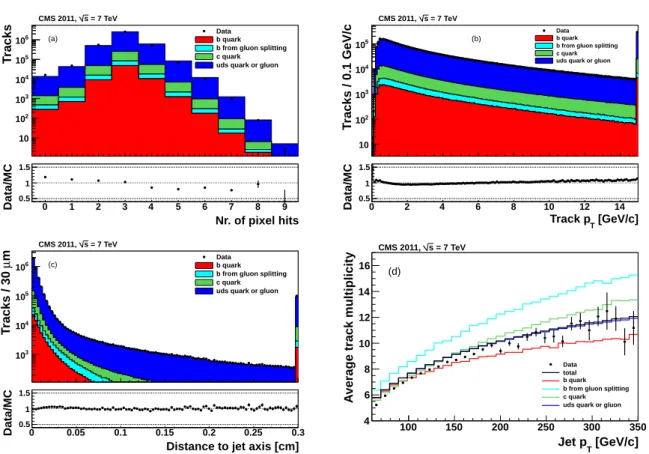
Properties of the tracks and the average multiplicity after the selection (except for the vari-able plotted) are shown in Fig. 1. The uncertainties shown in this and all following figures are statistical unless otherwise stated. The data were recorded with a prescaled jet trigger in the second part of 2011 when the number of pileup events was highest. The jet pT threshold
was 60 GeV/c. The distributions show satisfactory agreement with the expectations from sim-ulation. The track multiplicity and the lower part of the momentum spectrum are particularly sensitive to the modelling of the particle multiplicity and kinematics by the Monte Carlo gener-ator, as are other distributions such as the number of hits in the innermost pixel layers. Detector effects that are not modelled by the simulation, such as the dynamic readout inefficiency in the pixel system, can also contribute to the remaining discrepancies. In Fig. 1 and the following figures, simulated events with gluon splitting to bb are shown as a special category. The b jets in these events tend to be close in space and can be inadvertently merged by the clustering algorithm, resulting in a higher average track multiplicity per jet.
The combinatorial complexity of the reconstruction of the decay points (secondary vertices) of b or c hadrons is more challenging in the presence of multiple proton-proton interactions. In order to minimize this complexity a different track selection is applied. Tracks must be within a cone of∆R = 0.3 around the jet axis with a maximal distance to this axis of 0.2 cm and pass a “high-purity” criterion [32]. The “high-purity” criterion uses the normalized χ2 of the track
fit, the track length, and impact parameter information to optimize the purity for each of the iterations in track reconstruction. The vertex finding procedure begins with tracks defined by this selection and proceeds iteratively. A vertex candidate is identified by applying an adaptive vertex fit [31], which is robust in the presence of outliers. The fit estimates the vertex position and assigns a weight between 0 and 1 to each track based on its compatibility with the vertex. All tracks with weights>0.5 are then removed from the sample. The fit procedure is repeated until no new vertex candidate can be found. In the first iteration the interaction region is used as a constraint in order to identify the prompt tracks in the jet. The subsequent iterations produce decay vertex candidates.
4.2 Identification using track impact parameters
The impact parameter of a track with respect to the primary vertex can be used to distinguish the decay products of a b hadron from prompt tracks. The IP is calculated in three dimensions by taking advantage of the excellent resolution of the pixel detector along the z axis. The im-pact parameter has the same sign as the scalar product of the vector pointing from the primary vertex to the point of closest approach with the jet direction. Tracks originating from the decay of particles travelling along the jet axis will tend to have positive IP values. In contrast, the impact parameters of prompt tracks can have positive or negative IP values. The resolution of the impact parameter depends strongly on the pT and η of a track. The impact parameter
significance SIP, defined as the ratio of the IP to its estimated uncertainty, is used as an
observ-able. The distributions of IP values and their significance are shown in Fig. 2. In general, good agreement with simulation is observed with the exception of a small difference in the width of
nr. of pixel hits 0 1 2 3 4 5 6 7 8 9 T ra c k s 10 2 10 3 10 4 10 5 10 6 10 Data b quark b from gluon splitting c quark uds quark or gluon = 7 TeV s CMS 2011, (a) Nr. of pixel hits 0 1 2 3 4 5 6 7 8 9 Data/MC 0.5 1 1.5 track pT 0 2 4 6 8 10 12 14 T ra c k s / 0 .1 G e V /c 10 2 10 3 10 4 10 5 10 Data b quark b from gluon splitting c quark uds quark or gluon = 7 TeV s CMS 2011, (b) [GeV/c] T Track p 0 2 4 6 8 10 12 14 Data/MC 0.5 1 1.5
distance to jet axis
0 0.05 0.1 0.15 0.2 0.25 0.3 m µ T ra c k s / 3 0 3 10 4 10 5 10 6 10 Data b quark b from gluon splitting c quark uds quark or gluon = 7 TeV
s CMS 2011,
(c)
Distance to jet axis [cm]
0 0.05 0.1 0.15 0.2 0.25 0.3 Data/MC 0.5 1 1.5 [GeV/c] T Jet p 100 150 200 250 300 350 A v e ra g e t ra c k m u lt ip li c it y 4 6 8 10 12 14 16 Data total b quark b from gluon splitting c quark uds quark or gluon
= 7 TeV s CMS 2011,
(d)
Figure 1: Track properties after basic selection (except for the variable plotted): (a) number of hits in the pixel system, (b) transverse momentum, (c) distance to the jet axis. The average number of tracks passing the basic selection is shown in (d) as a function of the transverse mo-mentum of the jet. In (a)–(c) the distributions from simulation have been normalized to match the counts in data. The filled circles correspond to data. The stacked, coloured histograms indicate the contributions of different components from simulated multijet (“QCD”) samples. Simulated events involving gluon splitting to b quarks (“b from gluon splitting”) are indicated separately from the other b production processes (“b quark”). In each histogram, the rightmost bin includes all events from the overflow. The sample corresponds to a trigger selection with jet pT>60 GeV/c.
the core of the IP significance distribution.
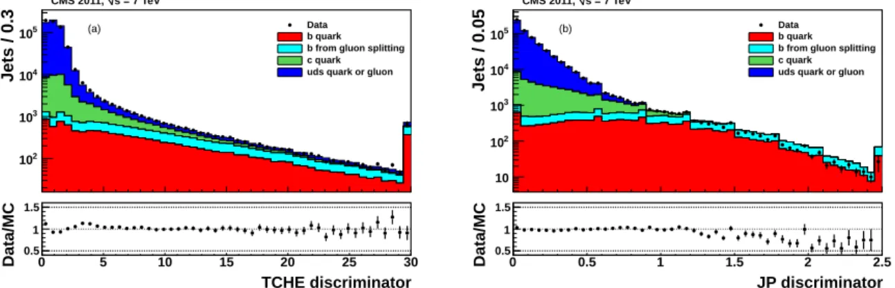
By itself the impact parameter significance has discriminating power between the decay prod-ucts of b and non-b jets. The Track Counting (TC) algorithm sorts tracks in a jet by decreasing values of the IP significance. Although the ranking tends to bias the values for the first track to high positive IP significances, the probability to have several tracks with high positive values is low for light-parton jets. Therefore the two different versions of the algorithm use the IP signif-icance of the second and third ranked track as the discriminator value. These two versions of the algorithm are called Track Counting High Efficiency (TCHE) and Track Counting High Purity (TCHP), respectively. The distribution of the TCHE discriminator is shown in Fig. 3 (a). A natural extension of the TC algorithms is the combination of the IP information of several tracks in a jet. Two discriminators are computed from additional algorithms. The Jet Probabil-ity (JP) algorithm uses an estimate of the likelihood that all tracks associated to the jet come from the primary vertex. The Jet B Probability (JBP) algorithm gives more weight to the tracks with the highest IP significance, up to a maximum of four such tracks, which matches the
av-4.2 Identification using track impact parameters 7 -0.1 -0.05 0 0.05 0.1 m µ T ra c k s / 2 0 2 10 3 10 4 10 5 10 Data b quark b from gluon splitting c quark uds quark or gluon = 7 TeV s CMS 2011, (a) 3D IP [cm] -0.1 -0.05 0 0.05 0.1 Data/MC 0.5 1 1.5 3D IP significance -30 -20 -10 0 10 20 30 T ra c k s / 0 .7 2 10 3 10 4 10 5 10 6 10 Data b quark b from gluon splitting c quark uds quark or gluon = 7 TeV s CMS 2011, (b) 3D IP significance -30 -20 -10 0 10 20 30 Data/MC 0.5 1 1.5
Figure 2: Distributions of (a) the 3D impact parameter and (b) the significance of the 3D impact parameter for all selected tracks. Selection and symbols are the same as in Fig. 1. Underflow and overflow are added to the first and last bins, respectively.
erage number of reconstructed charged particles from b-hadron decays. The estimate for the likelihood, Pjet, is defined as
Pjet =Π· N−1
∑
i=0 (−lnΠ)i i! with Π= N∏
i=1 max(Pi, 0.005), (1)where N is the number of tracks under consideration and Pi is the estimated probability for
track i to come from the primary vertex [33, 34]. The Pi are based on the probability density
functions for the IP significance of prompt tracks. These functions are extracted from data for different track quality classes, using the shape of the negative part of the SIPdistribution.
Eight quality classes are defined for tracks with χ2/n.d.o.f<2.5, depending on the momentum (<8 or>8 GeV/c) and pseudorapidity (|η|within 0-0.8, 0.-1.6, 1.6-2.4 if there are at least three pixel hits or |η| < 2.4 if there are only two pixel hits). A ninth quality class is defined for tracks with χ2/n.d.o.f > 2.5. The cut-off parameter for P
i at 0.5% limits the effect of single,
poorly reconstructed tracks on the global estimate. The discriminators for the jet probability algorithms have been constructed to be proportional to −ln Pjet. The distribution of the JP
discriminator in data and simulation is shown in Fig. 3 (b).
TCHE discriminator 0 5 10 15 20 25 30 Jets / 0.3 2 10 3 10 4 10 5 10 Datab quark
b from gluon splitting c quark uds quark or gluon = 7 TeV s CMS 2011, (a) TCHE discriminator 0 5 10 15 20 25 30 Data/MC 0.5 1 1.5 JP discriminator 0 0.5 1 1.5 2 2.5 Jets / 0.05 10 2 10 3 10 4 10 5 10 Data b quark b from gluon splitting c quark uds quark or gluon = 7 TeV s CMS 2011, (b) JP discriminator 0 0.5 1 1.5 2 2.5 Data/MC 0.5 1 1.5
Figure 3: Discriminator values for (a) the TCHE and (b) the JP algorithms. Selection and sym-bols are the same as in Fig. 1. The small discontinuities in the JP distributions are due to the single track probabilities which are required to be greater than 0.5%.
3D flight significance 0 10 20 30 40 50 60 70 80 SV / 0.8 10 2 10 3 10 4 10 Data b quark b from gluon splitting c quark uds quark or gluon = 7 TeV
s CMS 2011,
(a)
3D SV flight distance significance
0 10 20 30 40 50 60 70 80 Data/MC 0.5 1 1.5 0 1 2 3 4 5 6 7 8 2 SV / 0.08 GeV/c 0 500 1000 1500 2000 Data b quark b from gluon splitting c quark uds quark or gluon = 7 TeV s CMS 2011, (b) ] 2 SV mass [GeV/c 0 1 2 3 4 5 6 7 8 Data/MC 0.5 1 1.5
Figure 4: Properties of reconstructed decay vertices: (a) the significance of the 3D secondary vertex (3D SV) flight distance and (b) the mass associated with the secondary vertex. Selection and symbols are the same as in Fig. 1.
4.3 Identification using secondary vertices
The presence of a secondary vertex and the kinematic variables associated with this vertex can be used to discriminate between b and non-b jets. Two of these variables are the flight distance and direction, using the vector between primary and secondary vertices. The other variables are related to various properties of the system of associated secondary tracks such as the multiplicity, the mass (assuming the pion mass for all secondary tracks), or the energy. Secondary-vertex candidates must meet the following requirements to enhance the b purity:
• secondary vertices must share less than 65% of their associated tracks with the pri-mary vertex and the significance of the radial distance between the two vertices has to exceed 3σ;
• secondary vertex candidates with a radial distance of more than 2.5 cm with respect to the primary vertex, with masses compatible with the mass of K0 or exceeding 6.5 GeV/c2 are rejected, reducing the contamination by vertices corresponding to the interactions of particles with the detector material and by decays of long-lived mesons;
• the flight direction of each candidate has to be within a cone of∆R<0.5 around the jet direction.
The Simple Secondary Vertex (SSV) algorithms use the significance of the flight distance (the ratio of the flight distance to its estimated uncertainty) as the discriminating variable. The algorithms’ efficiencies are limited by the secondary vertex reconstruction efficiency to about 65%. Similar to the Track Counting algorithms, there exist two versions optimized for different purity: the High Efficiency (SSVHE) version uses vertices with at least two associated tracks, while for the High Purity (SSVHP) version at least three tracks are required. In Fig. 4 the flight distance significance and the mass associated with the secondary vertex are shown.
A more complex approach involves the use of secondary vertices, together with track-based lifetime information. By using these additional variables, the Combined Secondary Vertex (CSV) algorithm provides discrimination also in cases when no secondary vertices are found, increas-ing the maximum efficiency with respect to the SSV algorithms. In many cases, tracks with an SIP > 2 can be combined in a “pseudo vertex”, allowing for the computation of a subset
of secondary-vertex-based quantities even without an actual vertex fit. When even this is not possible, a “no vertex” category reverts to track-based variables that are combined in a way similar to that of the JP algorithm.
4.4 Performance of the algorithms in simulation 9 0 1 2 3 4 5 Jets -2 10 -1 10 1 10 2 10 3 10 4 10 5 10 6 10 Data b quark b from gluon splitting c quark uds quark or gluon = 7 TeV s CMS 2011, (a) Nr. of secondary vertices 0 1 2 3 4 5 Data/MC 0.5 1 1.5 0 0.1 0.2 0.3 0.4 0.5 0.6 0.7 0.8 0.9 1 entries 2 10 3 10 4 10 5 10 Datab quark
b from gluon splitting c quark uds quark or gluon = 7 TeV s CMS 2011, (b) CSV discriminator 0 0.1 0.2 0.3 0.4 0.5 0.6 0.7 0.8 0.9 1 Data/MC 0.5 1 1.5
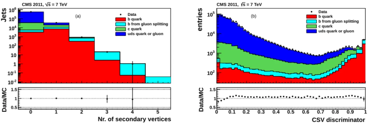
Figure 5: Distributions of (a) the secondary vertex multiplicity and (b) the CSV discriminator. Selection and symbols are the same as in Fig. 1.
The following set of variables with high discriminating power and low correlations is used (in the “no vertex” category only the last two variables are available):
• the vertex category (real, “pseudo,” or “no vertex”);
• the flight distance significance in the transverse plane (“2D”);
• the vertex mass;
• the number of tracks at the vertex;
• the ratio of the energy carried by tracks at the vertex with respect to all tracks in the jet;
• the pseudorapidities of the tracks at the vertex with respect to the jet axis;
• the 2D IP significance of the first track that raises the invariant mass above the charm threshold of 1.5 GeV/c2 (tracks are ordered by decreasing IP significance and the mass of the system is recalculated after adding each track);
• the number of tracks in the jet;
• the 3D IP significances for each track in the jet.
Two likelihood ratios are built from these variables. They are used to discriminate between b and c jets and between b and light-parton jets. They are combined with prior weights of 0.25 and 0.75, respectively. The distributions of the vertex multiplicity and of the CSV discriminator are presented in Fig. 5.
4.4 Performance of the algorithms in simulation
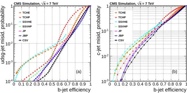
The performance of the algorithms described above is summarized in Fig. 6 where the pre-dictions of the simulation for the misidentification probabilities (the efficiencies to tag non-b jets) are shown as a function of the b-jet efficiencies. Jets with pT > 60 GeV/c in a sample of
simulated multijet events are used to obtain the efficiencies and misidentification probabilities. For loose selections with 10% misidentification probability for light-parton jets a b-jet tagging efficiency of ∼ 80–85% is achieved. In this region the JBP has the highest b-jet tagging effi-ciency. For tight selections with misidentification probabilities of 0.1%, the typical b-jet tagging efficiency values are ∼ 45–55%. For medium and tight selections the CSV algorithm shows the best performance. As can be seen in Fig. 6, the TC and SSV algorithms cannot be tuned to provide good performance for the whole range of operating points. Therefore two versions of these algorithms are provided, with the “high efficiency” version to be used for loose to medium operating points and the “high purity” version for tighter selections. Because of the
b-jet efficiency
0 0.1 0.2 0.3 0.4 0.5 0.6 0.7 0.8 0.9 1
udsg-jet misid. probability
-4 10 -3 10 -2 10 -1 10 1CMS Simulation, s = 7 TeV TCHE TCHP SSVHE SSVHP JP JBP CSV (a) b-jet efficiency 0 0.1 0.2 0.3 0.4 0.5 0.6 0.7 0.8 0.9 1
c-jet misid. probability
-3 10 -2 10 -1 10 1CMS Simulation, s = 7 TeV TCHE TCHP SSVHE SSVHP JP JBP CSV (b)
Figure 6: Performance curves obtained from simulation for the algorithms described in the text. (a) light-parton- and (b) c-jet misidentification probabilities as a function of the b-jet effi-ciency. Jets with pT >60 GeV/c in a sample of simulated multijet events are used to obtain the
efficiency and misidentification probability values.
non-negligible lifetime of c hadrons the separation of c from b jets is naturally more challenging. Due to the explicit tuning of the CSV algorithm for light-parton- and c-jet rejection it provides the best c-jet rejection values in the high-purity region.
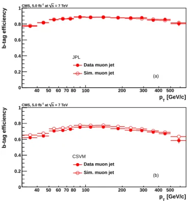
Figure 7 presents the efficiencies and misidentification probabilities as a function of jet pT and
pseudorapidity for the JPL and CSVM taggers. Two simulated samples are used: a QCD multi-jet sample with a multi-jet pTtrigger threshold of 60 GeV/c applied to the leading jet, and a tt sample.
Jets with pT > 30 GeV/c and |η| < 2.4 are considered in both cases. The b-jet identification efficiency is slightly larger in tt events at small jet pT (< 100 GeV/c) due to the presence of
more central jets. At large jet pT(>200 GeV/c), the presence of b and c jets from gluon splitting
explains the apparent higher identification efficiency in the QCD multijet sample. The b-jet efficiency and the c-jet misidentification probability rise with jet pTfor values below 100 GeV/c
and decrease above 200 GeV/c. This dependence is due to a convolution of the track impact pa-rameter resolution (which is larger at low pT), of the heavy-hadron decay lengths (which scale
with jet pT) and of the track-selection criteria. The misidentification probability for light-parton
jets rises continuously with jet pT due to the logarithmic increase of the number of particles
in jets and the higher fraction of merged hits in the innermost layers of the tracking system. However, both the identification efficiencies and misidentification probabilities stay roughly constant over most of the pixel detector acceptance.
4.5 Impact of running conditions on b-jet identification
All tagging algorithms rely on a high track identification efficiency and a reliable estimation of the track parameters and their uncertainties. These are both potentially sensitive to changes in the running conditions of the experiment. The robustness of the algorithms with respect to the misalignment of the tracking system and an increase in the density of tracks due to pile up, which are the most important of the changes in conditions, has been studied.
4.5 Impact of running conditions on b-jet identification 11 [GeV/c] T p 40 50 60 100 200 300 400
efficiency or misid. prob.
0 0.2 0.4 0.6 0.8 1 JPL: QCD events
b quark c quark uds quark or gluon
eventst
t
b quark c quark uds quark
= 7 T e V s CMS Simulation, (a) | η | 0 0.5 1 1.5 2
efficiency or misid. prob.
0 0.2 0.4 0.6 0.8 1 JPL: QCD events
b quark c quark uds quark or gluon
eventst
t
b quark c quark uds quark
= 7 T e V s CMS Simulation, (c) [GeV/c] T p 40 50 60 100 200 300 400
efficiency or misid. prob.
0 0.1 0.2 0.3 0.4 0.5 0.6 0.7 0.8 CSVM: QCD events b quark c quark 10) ×
uds quark or gluon (
eventst t b quark c quark 10) × uds quark ( = 7 T e V s CMS Simulation, (b) | η | 0 0.5 1 1.5 2
efficiency or misid. prob.
0 0.1 0.2 0.3 0.4 0.5 0.6 0.7 0.8 CSVM: QCD events b quark c quark 10) ×
uds quark or gluon (
eventst t b quark c quark 10) × uds quark ( = 7 T e V s CMS Simulation, (d) Figur e 7: Ef ficiency for b-jets and misidentification pr obabilities for c and light-parton jets of the (a, c) JPL and (b, d) CSVM taggers as a function of (a, b) je t pT and (c, d) jet pseudorapidity in QCD multijet events (filled symbols) and tt events (open symbols). A trigger thr eshold of pT > 60 Ge V / c is applied to the leading jet in the QCD event s. Jets with pT > 30 Ge V / c and | η | < 2.4 ar e used in both samples. In (a) and (b), the rightmost bins includes all jets with pT > 500 Ge V / c. For the CSVM tagger , the misidentification pr obability for light partons is scaled up by a factor of ten.
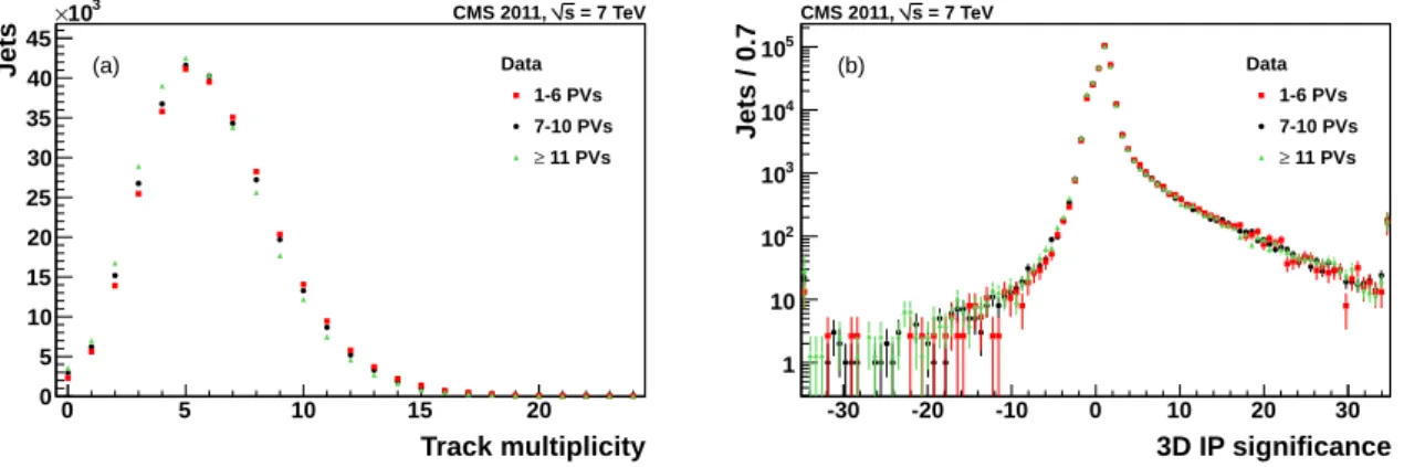
Track multiplicity 0 5 10 15 20 Jets 0 5 10 15 20 25 30 35 40 45 3 10 × Data 1-6 PVs 7-10 PVs 11 PVs ≥ = 7 TeV s CMS 2011, (a) 3D IP significance -30 -20 -10 0 10 20 30 Jets / 0.7 1 10 2 10 3 10 4 10 5 10 Data 1-6 PVs 7-10 PVs 11 PVs ≥ = 7 TeV s CMS 2011, (b)
Figure 8: (a) the number of tracks associated with the selected jets for three ranges of primary vertex (PV) multiplicity. (b) the IP significance of the second-most significant track, for the three ranges of primary vertex multiplicity. The selection is the same as in Fig. 1. The distributions are normalized to the event count for 1–6 PV range. Underflow and overflow entries are added to the first and last bins, respectively.
minimum bias collisions [35, 36], and is regularly monitored. During the 2011 data taking, the most significant movements were between the two halves of the pixel barrel detector, where discrete changes in the relative z position of up to 30 µm were observed. The sensitivity of b-jet identification to misalignment was studied on simulated t¯t samples. With the current estimated accuracy of the positions of the active elements, no significant deterioration is observed with respect to a perfectly aligned detector. The effect of displacements between the two parts of the pixel barrel detector was studied by introducing artificial separations of 40, 80, 120, and 160 µm in the detector simulation. The movements observed in 2011 were not found to cause any significant degradation of the performance.
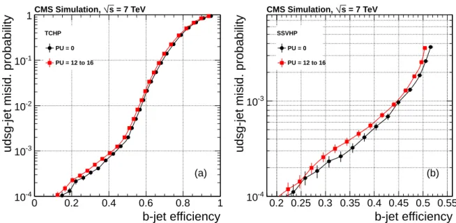
Because of the luminosity profile of the 2011 data, the number of proton collisions taking place simultaneously in one bunch crossing was of the order of 5 to 20 depending on the time period. Although these additional collisions increase the total number of tracks in the event, the track selection is able to reject tracks from nearby primary vertices. The multiplicity distribution of selected tracks is almost independent of the number of primary vertices, as shown in Fig. 8 (a). There is an indication of a slightly lower tracking efficiency in events with high pileup. The rejection of the additional tracks is mainly due to the requirement on the distance of the tracks with respect to the jet axis. This selection criterion is very efficient for the rejection of tracks from pileup. The reconstruction of track parameters is hardly affected. The distribution of the second-highest IP significance is stable, as shown in Fig. 8 (b). The impact of high pileup on the b-jet tagging performance is illustrated in Fig. 9. This shows the light-parton misidentification probability versus the b-jet tagging efficiency for the TCHP and SSVHP algorithms. In order to focus on the changes due to the b-jet tagging algorithms, the performance curves have been compared using a jet pTthreshold of 60 GeV/c at the generator level. The changes are small and
concentrated in the regions of very high purity.
5
Efficiency measurement with multijet events
For the b-jet tagging algorithms to be used in physics analyses, it is crucial to know the effi-ciency for each algorithm to select genuine b jets. There are a number of techniques that can be applied to CMS data to measure the efficiencies in situ, and thus reduce the reliance on simula-tions. If event distributions from MC simulation match those observed in data reasonably well,
5.1 Efficiency measurement with kinematic properties of muon jets 13
b-jet efficiency
0 0.2 0.4 0.6 0.8 1
udsg-jet misid. probability
-4 10 -3 10 -2 10 -1 10 1CMS Simulation, s = 7 TeV TCHP PU = 0 PU = 12 to 16 (a) b-jet efficiency 0.2 0.25 0.3 0.35 0.4 0.45 0.5 0.55
udsg-jet misid. probability
-4 10 -3 10 = 7 TeV s CMS Simulation, SSVHP PU = 0 PU = 12 to 16 (b)
Figure 9: Light-parton misidentification probability versus b-jet tagging efficiency for jets with pT > 60 GeV/c at generator level for the (a) TCHP and (b) SSVHP algorithms for different
pileup (PU) scenarios.
then the simulation can be used for a wide range of topologies after applying corrections deter-mined from specific data samples. Corrections can be applied to simulated events using a scale factor SFb, defined as the ratio of the efficiency measured with collision data to the efficiency found in the equivalent simulated samples, using MC generator-level information to identify the jet flavour. Furthermore, the measurement techniques used for data are also applied to the simulation in order to validate the different algorithms.
Some efficiency measurements are performed using samples that include a jet with a muon within∆R =0.4 from the jet axis (a “muon jet”). Because the semileptonic branching fraction of b hadrons is significantly larger than that for other hadrons (about 11%, or 20% when b →
c → ` cascade decays are included), these jets are more likely to arise from b quarks than from another flavour. Muons are identified very efficiently in the CMS detector, making it straightforward to collect samples of jets with at least one muon. These muons can be used to measure the performance of the lifetime-based tagging algorithms, since the efficiencies of the muon- and lifetime-based b-jet identification techniques are largely uncorrelated. Sections 5.1 and 5.2 describe efficiency measurements that use muon jets, while the technique of Section 5.3 makes use of a more generic dijet sample. The results are given in Section 7.
5.1 Efficiency measurement with kinematic properties of muon jets
Due to the large b-quark mass, the momentum component of the muon transverse to the jet axis, prel
T , is larger for muons from b-hadron decays than for muons in light-parton jets or from
charm hadrons. This component is used as the discriminant for the “PtRel” method. In addi-tion, the impact parameter of the muon track, calculated in three dimensions, is also larger for b hadrons than for other hadrons. This parameter is used as the discriminant for the “IP3D” method. Both of these variables can thus be used as a discriminant in the b-jet tagging efficiency determination. In both cases, the discriminating power of the variable depends on the muon jet pT. The muon prelT (IP) distributions provide better separation for jets with pTsmaller (greater)
than about 120 GeV/c. The PtRel and IP3D methods rely on fits to the prel
T [37] and muon IP
background.
In the two methods, the prel
T and IP spectra for muon jets are modelled using simulated
distri-butions that represent the spectra expected for different jet flavours to obtain the b-jet content of the sample. The efficiency for a particular tagger is obtained by measuring the fraction of muon jets that satisfy the requirements of the tagger. To make the treatment of the statistical uncertainty more straightforward, the muon jet sample is separated into those jets that satisfy and those that fail the requirements of the tagger. These jets are referred to as “tagged” and “untagged.”
A dijet sample with high b-jet purity is obtained by requiring that events have exactly two re-constructed jets: the muon jet as defined above and another jet fulfilling the TCHPM b-jet tag-ging criterion (the “medium” operating point for the TCHP algorithm). Simulated MC events are used to establish prelT and IP spectra for muon jets resulting from the fragmentation of b, c, and light partons. Muons in light-parton jets mostly arise from the decay of charged pions or kaons and from misidentified muons or hadronic punch-through in the calorimeters, effects that might not be modelled well in the simulation. The spectra for light-parton jets from simu-lation can be validated against control samples of collision data. In Fig. 10 the distributions of prelT and ln(|IP|[cm])derived from the simulation are compared to the ones obtained for tracks in inclusive jet data by applying the same kinematic selection and track reconstruction quality requirements as for the muon candidates. In order to measure the ability of the simulation to model the investigated spectra, we apply the same procedure to a sample of simulated inclu-sive jet events. The spectra derived for low-pT muons from light-parton jets in simulation are
corrected by multiplying them with the ratio of shapes of the inclusive distributions obtained in data and simulation on a bin-by-bin basis.
[GeV/c] rel T p 0 0.5 1 1.5 2 2.5 3 3.5 4 4.5 5 Arbitrary units 0 0.02 0.04 0.06 0.08 0.1 0.12 MC light MC, any tracks Data, any tracks MC light scaled = 7 TeV s at -1 CMS, 5.0 fb (a) ln(|IP|[cm]) -10 -9 -8 -7 -6 -5 -4 -3 -2 -1 0 Arbitrary units 0 0.02 0.04 0.06 0.08 0.1 0.12 MC light MC, any tracks Data, any tracks MC light scaled = 7 TeV s at -1 CMS, 5.0 fb (b)
Figure 10: Comparison of distributions of (a) muon prelT for jets with pT between 80 and
120 GeV/c and (b) ln(|IP|[cm])for jets with pTbetween 160 and 320 GeV/c for muons in
simu-lated light-parton jets (“MC light”), tracks from simusimu-lated inclusive jet events (“any tracks”), tracks from data, and muons in simulated light-parton jets after corrections based on data (“MC light scaled”).
The fractions of each jet flavour in the dijet sample are extracted with a binned maximum like-lihood fit using prelT and IP templates for b, c and light-parton jets derived from simulation or inclusive jet data. The fits are performed independently in the tagged and untagged subsam-ples of the muon jets. Results of representative fits are shown in Figs. 11 and 12.
From each fit the fractions of b jets ( fbtag, fbuntag) are extracted from the data. With these fractions and the total yields of tagged and untagged muon jets (Ndatatag , Ndatauntag), the number of b jets in
5.1 Efficiency measurement with kinematic properties of muon jets 15 [GeV/c] rel T p 0 0.5 1 1.5 2 2.5 3 3.5 4 4.5 5 Jets / 0.2 GeV/c 0 1000 2000 3000 4000 5000 6000 JPL tagged Data b jets light-parton + c jets = 7 TeV s at -1 CMS, 5.0 fb (a) [GeV/c] rel T p 0 0.5 1 1.5 2 2.5 3 3.5 4 4.5 5 Jets / 0.2 GeV/c 0 1000 2000 3000 4000 5000 CSVM tagged Data b jets light-parton + c jets = 7 TeV s at -1 CMS, 5.0 fb (b) [GeV/c] rel T p 0 0.5 1 1.5 2 2.5 3 3.5 4 4.5 5 Jets / 0.2 GeV/c 0 1000 2000 3000 4000 5000 JPL untagged Data b jets light-parton + c jets = 7 TeV s at -1 CMS, 5.0 fb (c) [GeV/c] rel T p 0 0.5 1 1.5 2 2.5 3 3.5 4 4.5 5 Jets / 0.2 GeV/c 0 1000 2000 3000 4000 5000 6000 7000 CSVM untagged Data b jets light-parton + c jets = 7 TeV s at -1 CMS, 5.0 fb (d)
Figure 11: Fits of the summed b and non-b templates, for simulated muon jets, to the muon prelT distributions from data. (a) and (c) show the results for muon jets that pass (tagged) or fail (untagged) the b-jet tagging criteria of the JPL method, respectively. (b) and (d) are the equivalent plots for the CSVM method. The muon jet pTis between 80 and 120 GeV/c.
ln(|IP|[cm]) -10 -9 -8 -7 -6 -5 -4 -3 -2 -1 0 Jets / 0.4 0 500 1000 1500 2000 2500 3000 3500 4000 JPL tagged Data b jets c jets light-parton jets = 7 TeV s at -1 CMS, 5.0 fb (a) ln(|IP|[cm]) -10 -9 -8 -7 -6 -5 -4 -3 -2 -1 0 Jets / 0.4 0 500 1000 1500 2000 2500 3000 CSVM tagged Data b jets c jets light-parton jets = 7 TeV s at -1 CMS, 5.0 fb (b) ln(|IP|[cm]) -10 -9 -8 -7 -6 -5 -4 -3 -2 -1 0 Jets / 0.4 0 1000 2000 3000 4000 5000 JPL untagged Data b jets c jets light-parton jets = 7 TeV s at -1 CMS, 5.0 fb (c) ln(|IP|[cm]) -10 -9 -8 -7 -6 -5 -4 -3 -2 -1 0 Jets / 0.4 0 1000 2000 3000 4000 5000 6000 7000 CSVM untagged Data b jets c jets light-parton jets = 7 TeV s at -1 CMS, 5.0 fb (d)
Figure 12: Same as Fig. 11 using the ln(|IP|[cm])distributions. The muon jet pT is between 160
these samples are calculated, and the efficiency εtagb for tagging b jets in the data is inferred: εtagb = f tag b ·N tag data
fbtag·Ndatatag + fbuntag·Ndatauntag . (2)
To obtain SFb, the efficiency for tagging b jets in the simulation is obtained from jets that have
been identified as b jets with MC generator-level matching.
5.2 Efficiency measurement with the System8 method
The “System8” method [38, 39] is applied to events with a muon jet and at least one other, “away-tag”, jet. The muon jet is used as a probe. The reference lifetime tagger and a supple-mentary prelT -based selection are tested on this jet. The away-tag jet is tested with a separate lifetime tagger. There are eight quantities that can be counted from the full data sample. The quantities depend on the number of passing or failing tags. A set of equations correlates these eight quantities with the tagging efficiencies.
A muon jet can be tagged as a b jet using either a lifetime tagger, or by requiring that the muon has large prel
T . In this analysis, the requirement is prelT > 0.8 GeV/c. These two tagging criteria
have efficiencies εtagb and εPtRelb , respectively, for b jets. The third tagging criterion is the require-ment that another jet in the event passes also a lifetime-based tagger. This last requirerequire-ment defines the “away-tag sample”. It enriches the b content of the events, and thus makes it more likely that the muon jet is a b jet. Correlations between the efficiencies of the two tagging crite-ria are estimated from simulation. As prelT provides less discrimination between jet flavours at higher jet energies, the System8 method loses sensitivity for jet pT >120 GeV/c.
With these criteria eight quantities are measured. The four quantities for the muon jets are: the total number of muon jets in the sample n, the number of muon jets that pass the lifetime-tagging criterion ntag, the number of muon jets that pass the prelT requirement nPtRel, and the number of muon jets that pass both criteria ntag,PtRel. Likewise, the four quantities for the away-tag sample are labelled p, ptag, pPtRel, ptag,PtRel. The away-tag jets are tagged with the TCHPL criterion.
The full muon jet sample, n, and the away-tag sample, p, are each composed of an unknown mix of b and non-b jets. The non-b jets are labelled “c`”. The muon sample thus comprises nband nc`, and the away-tag sample, pb and pc`. The efficiencies of the two tagging criteria
on b jets (εtagb , εPtRelb ) and on non-b jets (εtagc` , εPtRelc` ) are also unknown, for a total of eight un-known quantities. Thus, a system of eight equations can be written that relates the measurable quantities to the unknowns:
n = nb+nc` , p = pb+pc` , ntag = εtagb nb+εtagc` nc` ,
ptag = βtagεtagb pb+αtagεtagc` pc` , (3) nPtRel = εPtRelb nb+εPtRelc` nc`,
pPtRel = βPtRel εPtRelb pb+αPtRel εPtRelc` pc` ,
ntag,pTrel = βn εtag
b ε
PtRel
b nb+αnεtagc` εPtRelc` nc` ,
ptag,pTrel = βp εtag
5.3 Efficiency measurement using a reference lifetime algorithm 17
The method assumes that the efficiencies for a combination of tagging criteria are factorizable. Thus eight correlation factors are introduced to solve the system of equations: αtag, βtag, αPtRel,
βPtRel, αn, βn, αp, and βp. These factors are obtained from the simulation as a function of the
muon jet pTand|η|. The factors α and β are determined for non-b and b jets, respectively. The superscripts “tag” and “PtRel” of α and β indicate the efficiency ratio of the p to the n samples for the lifetime and prelT criteria. The superscripts “n” and “p” refer to the correlation between the two tagging efficiencies, “tag” and “PtRel”, in the n and p samples.
The simulation predicts that the correlation coefficients typically range between 0.95 and 1.05 for those associated with the b-jet tagging efficiencies, and between 0.7 and 1.2 for those associ-ated with the c+`-tagging efficiencies. A numerical computation is applied to solve the system of eight equations in the data to determine the eight unknowns, thus simultaneously determin-ing the taggdetermin-ing efficiencies and flavour contents of both the full and away-tag samples.
5.3 Efficiency measurement using a reference lifetime algorithm
While muon prelT provides less discrimination power between jet flavours at large jet pT, the
lifetime-based algorithms described in Sections 4.2 and 4.3 (TCHE, TCHP, JP, JBP, SSVHE, SSVHP and CSV) retain their sensitivity to distinguish different jet flavours. In particular, the discriminant for the jet probability algorithm has different distributions for different jet flavours for jet momenta in the range 30< pT <700 GeV/c. The JP algorithm can be calibrated
directly with data. Tracks with negative impact parameter are used to compute the probability that those tracks come from the primary vertex. The same calibration is performed separately in simulated samples. As a result, the JP algorithm serves as a reference for estimating the frac-tion of b jets in a data sample, and also for estimating the fracfrac-tion of b jets in a subsample that has been selected by an independent tagging algorithm. In this manner the efficiency of the independent algorithm can be measured. This method is called the lifetime tagging method (“LT”). It can be performed on both inclusive and muon jet samples. The resulting scale factors are compared to obtain an estimate of the systematic uncertainty.
The efficiency measurement is performed in inclusive jet events in which at least one jet must be above a given pTthreshold, and separately in dijet events in which at least one jet is a muon
jet. To increase the fraction of b jets in the inclusive sample, an additional jet tagged by the JPM algorithm is also required. The sample with muon jets is already sufficiently enriched in b jets by the muon requirement. The same set of samples can be established with simulated events, so that the true tagging efficiency can be measured there and a scale factor computed.
Because a value of the JP discriminant can be defined for jets that have as few as one track with a positive impact parameter significance, the discriminant can be calculated for most b jets, regardless of their pT. The fraction of b jets that have JP information, Cb, rises from about 0.91
at pT =20 GeV/c to more than 0.98 for pT>50 GeV/c.
Figure 13 shows the JP discriminant distributions in the muon jet sample and the inclusive sample, before and after tagging the jets with an independent tagger, in this case the CSVM tagger. Also shown is a fit to the distributions using JP-discriminant templates derived from simulations of b, c, and light-parton jets. The normalization of the relative flavour fractions fb, fc and flightis left free, with the constraint that fb+ fc+ flight =1. The b-jet tagging efficiency
is the ratio of the number of b jets that are tagged by the independent tagger to the number of b jets before the tagging. The numbers are calculated using the fit. The b-jet tagging efficiency is corrected for the fraction of jets that have JP information.
εtagb = Cb
·fbtag·Ndatatag
fbbefore tag·Ndatabefore tag, (4)
where the superscripts “before tag” and “tag” refer to the samples before and after application of the tagging criterion.
JP discriminator 0 0.5 1 1.5 2 2.5 Jets / 0.1 2 10 3 10 4 10 Data fit b jets c jets light-parton jets = 7 TeV s at -1 CMS, 5.0 fb (a) JP discriminator 0 0.5 1 1.5 2 2.5 Jets / 0.1 2 10 3 10 Data fit b jets c jets jets light-parton = 7 TeV s at -1 CMS, 5.0 fb (b) JP discriminator 0 0.5 1 1.5 2 2.5 Jets / 0.1 10 2 10 3 10 4 10 5 10 Data fit b jets c jets light-parton jets = 7 TeV s at -1 CMS, 5.0 fb (c) JP discriminator 0 0.5 1 1.5 2 2.5 Jets / 0.1 10 2 10 3 10 Data fit b jets c jets jets light-parton = 7 TeV s at -1 CMS, 5.0 fb (d)
Figure 13: Fits of the summed b, c and light-parton templates, for simulated jets, to the JP-discriminant distributions from data. (a) and (b) show the results for muon jets before and after identification with the CSVM tagger, respectively. (c) and (d), the equivalent plots for inclusive jets. The black line is the sum of the contributions from the templates. The jet pTis in
the range 260< pT <320 GeV/c. Overflows are displayed in the rightmost bins.
Examples of the efficiencies measured for the JPL and CSVM taggers are shown in Fig. 14. In both cases the results from simulation are close to those obtained from data.
This technique cannot be used to measure the efficiency of the JP algorithm itself, as the JP discriminant is used in the fit to determine the b-jet content of the sample. However, the CSV discriminant, which is mostly based on information from secondary vertices, can be used in its place to determine the flavour content. More than 90% of jets have CSV information, as is the case with the JP discriminant. But unlike the JP discriminant, the CSV discriminant cannot be calibrated solely with the data. To remedy this, the CSV discriminant is used to estimate
5.4 Systematic uncertainties on efficiency measurements 19 [GeV/c] T p 40 50 60 70 80 100 200 300 400 500 b-tag efficiency 0 0.2 0.4 0.6 0.8 1 JPL
Data muon jet Sim. muon jet = 7 TeV s at -1 CMS, 5.0 fb (a) [GeV/c] T p 40 50 60 70 80 100 200 300 400 500 b-tag efficiency 0 0.2 0.4 0.6 0.8 1 CSVM
Data muon jet Sim. muon jet = 7 TeV s at -1 CMS, 5.0 fb (b)
Figure 14: Efficiencies for the identification of b-jets measured for (a) the JPL and (b) the CSVM tagger with the LT method in the muon jet sample. Filled and open circles correspond to data and simulation, respectively.
the tagging efficiency of the TC algorithms. By comparing these results to those using the JP discriminant, the bias due to using the CSV discriminant is determined to be (0–2%, 4–6%, 6– 9%) for the (loose, medium, tight) operating points. The efficiencies and scale factors for the JP algorithm are corrected for these biases.
5.4 Systematic uncertainties on efficiency measurements
Several systematic uncertainties affect the measurement of the b-jet tagging efficiency. Some are common to all four methods (PtRel, IP3D, System8, LT), some are common to a subset of them, and some are unique to a particular method.
Common systematic uncertainties for all methods:
• Pileup: The measured b-jet tagging efficiency depends on the number of pp colli-sions superimposed on the primary interaction of interest. The systematic uncer-tainty is computed by varying the average value of the pileup in data by 10% and calculating the difference in the values of SFbafter reweighting the simulation with
the modified distribution.
• Gluon splitting: Studies of angular correlation between b jets at the LHC [40] indi-cate that QCD events may have a larger fraction of gluon splitting into bb pairs than is assumed in the generation of the simulation. A study was carried out with the MC sample where the number of events with gluon splitting was artificially changed by 50%. Results obtained with this modified gluon splitting MC sample are then compared to those with the original sample. The observed deviation is quoted as a systematic uncertainty.
• Muon pTµ: The central value of the b-jet tagging efficiency is extracted from data with muon pµT >5 GeV/c. The choice of the selection affects the shape of the template distributions used in fits, and also the number of events used to measure the tagging efficiencies. The pTµ threshold is varied up to 9 GeV/c to test the sensitivity to this choice.
Common uncertainty for the PtRel, IP3D and System8 methods:
• Away-jet tagger: The dependency of the calculated b-jet tagging efficiency on the away-jet tagger is studied by comparing the results obtained by tagging the away jets with different variants of the TC algorithm (TCHEL, TCHEM, TCHPM). The measured SFbtends to increase when the away tag is tighter. The maximum devia-tion from the default away-jet tagger is taken as a systematic uncertainty.
Uncertainty unique to the PtRel method:
• Ratio of light-parton to charm jets in simulation: The shapes of the prelT and IP spectra for light-parton jets have been obtained from control samples in data, which minimizes the bias due to a mismodelling of the muon kinematics in the simula-tion. However, since the prel
T distribution in data is fitted with a sum of templates
for b jets and for c+udsg jets, uncertainties on the ratio between light-parton and charmed jets in the simulation must be considered. To do so, the predicted ratio is varied by ±20%, and the fit is repeated, taking the variation in the results as a systematic uncertainty. This uncertainty does not apply to the IP method, where a three-component fit is performed that determines the light-parton and charm con-tributions independently.
Uncertainties unique to the System8 method:
• Selection on prelT : One of the System8 criteria is a selection on the muon prelT >
0.8 GeV/c. In order to test the sensitivity to the b purity in the muon jet sample and the relative charm/light-parton fraction in the non-b background, this selection was changed from 0.5 to 1.2 GeV/c in the data. The correlation factors were recomputed accordingly in the simulation and the System8 method was applied again to the data in order to compute the b-jet tagging efficiency. The largest deviation observed from the central value is quoted as a systematic uncertainty.
• MC closure test: The b-jet tagging efficiency can be directly calculated from the simulated QCD muon-enriched sample, as the flavour of the jets at generator level is known. In this case, the efficiency can be measured by taking the number of identified true b jets over all true b jets. The resulting value is denoted as the MC truth b-jet tagging efficiency. The System8 method is also applied to this MC sample. The resulting b-jet tagging efficiencies are in good agreement with the MC truth, giving a negligible systematic uncertainty. (This systematic uncertainty does not appear for the other methods as they rely on template fits, making such a test trivial.) Uncertainties unique to the LT method:
• Fraction of b jets with JP information: The fraction of inclusive jets with JP infor-mation is well described by the simulation. As explained above, the number of b jets before tagging is measured by a fit to the JP distribution and corrected by the fraction Cbof b jets with JP information. A systematic uncertainty of half the resid-ual correction,(1−Cb)/(2Cb), is estimated from the simulation as a function of the

![Figure 12: Same as Fig. 11 using the ln (| IP |[ cm ]) distributions. The muon jet p T is between 160 and 320 GeV/c.](https://thumb-eu.123doks.com/thumbv2/123dok_br/15620022.1054845/17.892.131.737.682.1085/figure-fig-using-ip-distributions-muon-jet-gev.webp)