A general test for rule of thumb behavior

FUNDAÇÃO

GETUliO VARGAS

FGV

SEMINÁRIOS DE PESQUISA

ECONÔMICA DA EPGE

A general test for rule of Thumb behavior

JOÃO VICTOR ISSLER

(EPGE/FGV)

Data: 17/05/2007 (Quinta-feira)

Horário: 16h

Local:

Praia de Botafogo, 190- 11° andar Auditório n° 1

Coordenação:

A General Test for Rule-of-Thumb Behavior

Fabio A. Reis Gomes (CEPE-MG and IBMEC-MG)

João Victor lssler (EPGE- Getulio Vargas Foundation)

• Consumption is about 70% of GDP. Because of its the size, finding sub-optimal behavior in consumption decisions can cast a serious doubt on whether optimizing behavior is a framework applicable on an economy-wide scale, which, in turn, can challenge whether it is applicable at ali.

• Rule-of-Thumb behavior questions optimal behavior for consumption. Camp-bell and Mankiw(1989, 1990): 50% of ali U.S. consumers follow the rule-of-thumb behavior of consuming their current income, not their permanent

• In econometric tests, usually we have auxiliary assumptions whenever a specific hypothesis test is being conducted. In Campbell and Mankiw's case, the auxiliary assumption is the validity of the first-order log-linearized version of the Euler Equation for optimizing consumers. Rejecting the nu li that there is no rule-of-thumb behavior in this context may be due to the fact that the first-order log-linearized approximation of the Euler Equation

This Paper:

ｾ＠ We first show that, from a theoretical point-of-view, previous tests for Rule-of-Thumb behavior were inconsistent. This is based on an expansion of the basic non-linear euler equation for consumption.

ｾ＠ We then propose a novel framework that encampasses:

Possible Rule-of-Thumb behavior in consumption for a fixed proportion

À of the population. General test for À = O.

Possible habit formation for agents whose behavior is optimal.

This Paper (Contd.):

Motivation

e Huge discrepancy between time-series versus panel-data empirical studies in the consumption literature, suggesting the existence of aggregation bias.

e Mulligan(2002) uses a linear framework to study the effects of real return aggregation on intertemporal substitution. He comes up with new mea-sures for the after-tax return to aggregate capital, which are associated with reasonable and precise estimates of the intertemporal marginal rate of substitution in consumption.

M otivation ( Contd.)

Related Research

e Large early literature using time-series data on consumption: Ha11(1978, 1988), Flavin(1981, 1993), Mankiw(1981), Hansen and Singleton(1982, 1983, 1984), Mehra and Prescott(1985), Campbell (1987), Campbell and Deaton(1989), and Epstein and Zin(1991).

e Whole literature on Rule-of-Thumb behavior following H ali and Mishkin(1982) and subsequent work in Campbell and Mankiw (1989, 1990).

Related Research ( Contd.)

Theory

Pricing Equation:

lEt { Mt+lxi,t+l}

=

Pi,t' i

=

1, 2, ... , N, or (1)

IEt { Mt+lRi,t+l} = 1, i = 1, 2, ... , N, (2) where IEt( ·) denotes the conditional expectation given the information available at time t, Mt is the stochastic discount factor, Pi t denotes the price of the

'

i-th asset at time t, xi t+l denotes the payoff of the i-th asset in t

+

1,

Ri,t+l

=

ｸｾｴＫｬ＠

denotes 'the gross return of the i-th asset in

t

+

1, and N is the number

ｾｦ＠

assets in the economy.

Assumption 1: The Pricing Equation (2) holds.

• Assumption 1 is present, either implicitly or explicitly, in virtually ali stud-ies in macroeconomics dealing with asset pricing and intertemporal sub-stitution; see, e.g., Hansen and Singleton (1982, 1983, 1984), Mehra and

Prescott (1985), Epstein and Zin (1991), Attanasio and Browning (1995), Lettau and Ludvigson (2001) and Mulligan (2002).

• "Assumption" 2 is required because we will take logs of Mt. Ali CCAPM studies implicitly assume Mt >O, since Mt =

ｦＳｵｾＨＨ｣ｴＩＬ＠

>O, where ct is

Ct-1

consumption, {3 E (0, 1) and U1

Taylor expansion around x, with increment h, as follows:

h2ex+À(h)·h

ex+ hex

+

,

with .\(h) :IR-+ (0,

1),

or, (3) 2

ex+h

e h

_1+h+

h2eÀ(h)·h

_-

_'

₍₄₎

Let h= ln(MtRi,t) to obtain:

[ln(MtRi

t)]

2 eÀ(In(MtRi,t))·ln(MtRi,t)

MtRi,t

= 1

+

ln(MtRi,t)

+

'

2 . (5)

The behavior of

MtRi t

_,

is governed solely by that of

ln(MtRi t).

_' which moti-vates our next assumption.

Assumption 3: Let

Rt

= (R1 t, R2 t,

...

RN t)'

be an N x 1 vector

stack-' ' '

Higher-order term in (5):

z·

_2,t

_

_.

₂ l x [ln(M _.

_{t 2,t}

R· )] 2 e,\(ln(MtRi,t))·ln(MtRi,t).

Taking the conditional expectation of both sides of (5), imposing the Pricing Equation and rearranging terms, gives:

IEt-1 {

MtRi,t}

IEt-1 (

Zi,t)

1

+

IEt-1 {

ln(MtRi,t)}

+

IEt-1 (

zi,t)

,

or,

-IEt-1

{ln(MtRi,t)}.

(6)

(7)

Equation (7) shows that behavior of the conditional expectation of the higher order terms depends only on that of IEt-1

{ln(MtRi,t)

}.

Since

ln(MtRi,t)

is covariance stationary, IEt-1 (

Zi,t)

will be a linear function of the lagged

z· _2, t ₂

1

X [ln(M _{t 2,t} R· )] 2 e,\(ln(MtRi,t))·ln(MtRi,t)

>

_{_}

O

₁ implies ₁

Et-1 ( Zi,t) 'Yi,t 2

>

O.

2- ( 2 2 2 )' - ( )'

Let '"'ft

=

_{'Y1,t, 'Y2},t , ... , "YN,t and ct

=

E1,t, c2,t, ... , EN,t stack respec-tively the conditional means 'Y'i-t and the forecast errors Ei t = ln(MtRi

t)-(J' ' '

Et-1 {ln(MtRi,t) }.

From the definition of E:t and (6) we have:

Denoting

rt

= In

(Rt),

with elements ri,t· and mt = In (Mt) in (8), and using

IEt-1 ( zi,t) = -IEt-1 { ln(MtRi,t) }we get:

mt = -ri,t - IEt-1 ( Zi,t)

+

Ei,t, i = 1, 2, ... , N.

(9)

To connect this results with optimal consumption behavior we impose Mt =

{3

r

ＮＺｾｲｱｬ＠

.

.ó.ln (

ct)

= In

,B

+_!_r.

+

IE!t-1 ( Zi,t) Ei,t

• lEt-lJzi,t) captures the effect of the higher-order terms of the taylor

expan-sion. lt will be a function of the variables in the conditioning set used by the econometrician to compute

IEt-1 (-).

• Omission of

ＱｅｴＭｬｾｺｩＬｴＩ＠

in estimating (10) will generate an omitted-variable bias. The same is true of transformations of (10), in general.

• lf {

Mt+lRi,t+l}

is not log-Normal, using log-normality to solve for

Rule of Thumb Behavior

ｾ＠ Campbell and Mankiw (1989), following Hall and Mishkin(1982), proposed incorporating rule of thumb behavior to the optimizing model.

ｾ＠ Credit constrained consumers (Cushing, 1992) consume their current in-come, q t

=

Yl t

=

Àyt, where Yt is aggregate income.

' '

ｾ＠ À is the fraction of the total income which belongs to restricted consumers.

When À

=

1 there are only rule of thumb consumers and when À

=

O ali consumers follow optimizing behavior.

ｾ＠

Use weight À to compute llln (

ct)

rv Àllln ( C!,t)

+

(1 - À) llln ( C2,t) r

where

ct

=

q t

+

c2 t• and Yt

=

Yl t

+

Y2 t·

Rule of Thumb Behavior (Contd.)

Combine now

f),. I n ( c2,

t)

T

In (3

+

1 IEt-1

(zi,t)

E:i,t

4

/i,t

+

c/J -

-;j;'

i= 1, 2, ... , N, with,

I::!,. In (

ct)

r-v .\I::!,. In (C!,t)

+

(1-

.\)I::!,. In (c2,t), to get,

r-v .Xbs.ln

(Yt)

+

(1 -

.X) I::!,. In ( c2,t)

I::!,. In (

Ct)

ＭＭ］ＭＨ

Ｑ

ｾＭＮｘ｟［｟Ｉ＠

In (3

+

.\I::!,. In

(Yt)

+ (

1 - .X)

ri t

+ (

1 - .X)IEt-1

(zi

t)

cjJ cjJ ' cjJ . '

(1-

.X) .

-

E:i

t• ali _ｾＮ＠

Econometrics

bt..ln

(ct)

ＭＢＭＭＨ

Ｑ

ｾＭＮ｜ＭＧＭＩ＠

In ,8

+

.\bt..ln

(Yt)

+ (

1

-.\)ri t

+ (

1 - .\)lEt-1

(zi t)

4Y 4Y , 4Y ,

(1- .\)

- 4Y

Ei,t•

a 11 i.

• lf the term

Ｈ

Ｑ

ｾＬ｜ＩｬｅｴＭＱ＠

(zi,t)

is omitted, (almost?) every instrument used in the past to estimate this equation is invalid.

Econometrics ( Contd.)

.ô.ln (

ct)

｟Ｈ

Ｑ

ｾＭ￀｟Ｉ＠

In

,6

+

À.Õ.in

(Yt)

+ (

1

-À)

ri

t

+ (

1 - À)lEt-1

(zi

t)

cp

cp

'

cp

'

(1-

À)

- - é ' t

-

cp

'/,)

I i = 1, 2, ... ,

N.

Econometrics ( Contd.)

• Since, in principie, the number of assets can go to infinity, i.e., N --+ oo,

unless T --+ oo at rate N 2 , estimating the whole system is unfeasible.

Most of the literature did not take this issue seriously and opted to let

N = 2: a risky and a "riskless" asset.

• This procedure is suboptimal compared to estimating the system as a whole.

• An alternative to estimating the system as a whole is cross-sectional ag-gregation: Mulligan(2002), where in principie we do not throw away useful

information contained in ri t• i = 1, 2, ... , N.

Stylized Version of Mulligan(2002): Cross-sectionally aggregate

Llln

(ct)

ＭＧＭＨ

Ｑ

ｾＭ￀｟Ｉ＠

In

/3

+

Àilln

(yt)

+ (

1

-À)

Ti t

+ (

1 - À)IEt-1

(zi t)

ｾ＠ ｾ＠ ' ｾ＠ '

(1-

À)

.

.

- si t. ali ｾＮ＠ to obtam,

ｾ＠ '

Llln

(ct)

(1

-À)

In

/3

+

Àilln

(yt)

+ (

1

-À)

Tt

+ (

1 - À)IEt-1

(zt)

ｾ＠ ｾ＠ ｾ＠

(1 -

À)

ｾ＠ ct,

N

where

Tt

= N1 2:::::

Ti t

is the logarithmic return to aggregate capital,

zt

. 1 '

2=

1 N 1 N

N _{. 1 '} 2::::: Zi t. ct = N _{. 1 '} 2::::: éi t·

• Despite having a properly aggregated model, we have to take into account the term

Ｈｬｾ￀ＩｬｅｴＭｬ＠

(zt)-• lgnoring

Ｈｬｾ￀ＩｬｅｴＭＱ＠

(zt)

will also generate an omitted regressar problem under IV estimation, just as before. This happens whether or not À

=

O.

• Mulligan (2002) estimates the above regression imposing À = O.

Habit Formation

Consider now the extended CRRA utility, with habit formation,

U

(C[,

Cf-1)

=

(C[

-

f'Ct

1) 1-cp

1-cp

(11)

We let (o) stand for an optimizing consumer, and

(r)

stand for a credit-constrained consumer whose consumption is

ct;

= À.Yt· As before,

o+

r

ct=Ct Ct·

lnstead of considering the response of consumption to ali i = 1, 2, ... , N,

As in Weber(2002), solve for consumption of the optimizing consumer:

o- \

Ct - ct - AYt·

Habit Formation and General Rule-of-Thumb

Use the nonlinear euler equation as in Weber(2002). Use here the return to

aggregate capital. Then we encompass habit formation and rule-of-thumb in a

very general framework, with proper cross-sectional aggregation:

Et-1

( cf-1- 'fCf-2)

-<P-

f3

(

cf- 'Ycf-1)

-<P

h+

Rt]

+'Jf3

(

cf+1- 'Ycf)

-<P Rt

Substituting in

cf

= Ct- ÀYt we obtain:

[( ct-1 -

ÀYt-Ü -

'Y (

Ct-2 - ÀYt-2)]-<P

=

o,

(12)

Et-1

<

-{3 [(

ct-

Àyt) -

'Y ( ct-1 -

ÀYt-1)]-<P

h+

Rt]

t

= O. (13)

Obtaining (12) and (13): cross-sectional aggregation of:

E J ( cf-1 - --ycf-2)

-r/J

-

f3

(

cf - --ycf-1)

-r/J

[

'"Y

+

Ri,t]

t-1\ (

)-c/J

+--r/3

cf+1 - --ycf Ri,t

o

1, 2, ... , N. and,

.

'l

[(ct-1- ÀYt-1)- '"Y (ct-2- ÀYt-2)]-cP

O = Et-1

<

-j3 [(ct- Àyt)- '"Y (ct-1- ÀYt-Ü]-cP

[--r+

Ri,t]

+--r/3

[(

Ct+1 - ÀYt+1) - '"Y ( ct - Àyt)]-cP Ri,t

z = 1,2, ... ,N.

N N

where Rt

=

L

wi t ·Ri t• where

L

wi t

=

1, for ali

t.

. 1 ' ' . 1 '

H a bit Formation and Rule-of-Thumb ( contd.)

e lf there is no habit formation for the optimizing agent, "f = O, we obtain:

f3Et-1

I (

ct

-

ÀYt )

-c/J

Ct-1 - ÀYt-1 Rt

I

= 1

(14)

e lf there is no rule-of-thumb behavior, but there is habit formation, we obtain:

[ct-1 - "fCt-2]-c/J

Et-1 { -{3

[ct-

"fCt-1]-cP

[I+

Rt]

+"tf3 [ct+1 -

"tct]-cP

Rt

• lf there is neither rule-of-thumb nor habit formation, we obtain:

(

ct )

-c/J

f3Et-1

I

Rt

I

= 1.

Our Contribution:

e Regarding Weber(2002): we deal with cross-sectional aggregation of asset returns. No information is thrown away by limiting the number of as-sets. lndeed, we use Mulligan's(2002) capital rental rate after income and

property taxes as a measure of Rt.

e Regarding Mulligan(2002): We deal with non-linearity, Rule-of-Thumb, and Habit Formation.

ｾ＠ Cross sectional aggregation is properly taken care of by using the return to

aggregate capital and not a system of euler equations. This can be done beca use the euler equations are LINEAR on

Ri

t, i= 1, 2, ... ,

N,

despite

'

being non-linear on other variables and parameters.

ｾ＠ The nonlinear equation is key to our study. Estimating it directly allows

us to encompass ali high-order terms: General Rule-of-Thumb test and a General test for Habit Formation.

ｾ＠ The general model is ali in terms of observables. lt encampasses habit for-mation for the optimizing agent, ry

#-

O, as well as rule-of-thumb behavior for the credit-constrained consumer, À

#-

O.

ｾ＠ Estimation of (3, cjJ and À is performed using GMM. Habit formation and

Data

• Annual frequency form 1947 to 1997.

• US Nationallncome and Product Account (NIPA) and from the US Census Bureau: real disposable personal income, real consumption of nondurable and services and real consumption of non-durables, and population.

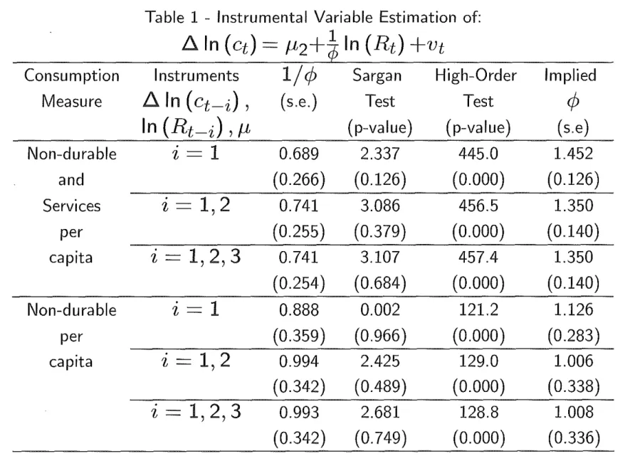
Table 1 - Instrumental Variable Estimation of:

f:::. In (

ct)

=

JL2+

à

In (

Rt) +vt

Consumption I nstru ments _1/c/J Sargan High-Order lmplied Measure L::::. In (

Ct-i)

,

(s.e.) Test Test _cP

In

(Rt-i), JL

(p-value) (p-value) (s.e)

Non-durable i= 1 0.689 2.337 445.0 1.452

and (0.266) (0.126) (0.000) (0.126)

Services i -_- 1 2 _' 0.741 3.086 456.5 1.350

per (0.255) (0.379) (0.000) (0.140)

capita i = 1, 2, 3 0.741 3.107 457.4 1.350 (0.254) (0.684) (0.000) (0.140)

Non-durable i= 1 0.888 0.002 121.2 1.126

per (0.359) (0.966) (0.000) (0.283)

capita i -_- 1 2

_'

0.994 2.425 129.0 1.006 (0.342) (0.489) (0.000) (0.338)

Table 2 - Instrumental Variable Estimation of:

.ó.ln (

ct)

= À.Ó.In

(yt)

+

(1- À)

ＨｾＱ＠

+

à

In

(Rt)

+

Vt)

Cons. lnst. (1- À)

/c/J

À Sargan Hi.-Order lmpl.

Meas. .ó.ln _(ct-i) (s.e.) (s.e.) Test Test cjJ

In

(Rt-i)

(p-val.) (p-val.) (s.e)

.ó. In

(yt_i) ,

c

Non-dur. i=1 0.496 0.199 2.680 104.2 1.616

and (0.322) (0.238) (0.102) (0.000)

Serv. i= 1, 2 0.389 0.300 3.570 151.0 1.799

per (0.264) (0.149) (0.467) (0.000)

capita i = 1, 2, 3 0.322 0.341 7.183 163.3 2.044

(0.255) (0.141) (0.410) (0.000)

Non-dur. i=1 0.667 0.238 0.001 14.90 1.125

per (0.691) (0.635) (0.980) (0.002)

capita i - 1 2 _-

_'

0.361 0.559 0.955 102.3 1.223

(0.374) (0.225) (0.917) (0.000)

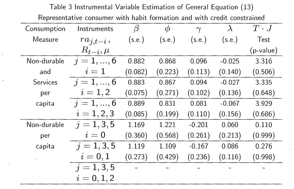
Table 3 Instrumental Variable Estimation of General Equation (13) Representative consumer with habit formation and with credit constrained

Consumption lnstruments j3

q;

"( À T·J

Measure _raj,t-i' (s.e.) ( s.e.) (s.e.) (s.e.) Test

Rt-i, f.L (p-value)

Non-durable j=1, ... ,6 0.882 0.868 0.096 -0.025 3.316

and i= 1 (0.082) (0.223) (0.113) (0.140) (0.506)

Services j=1, ... ,6 0.883 0.867 0.094 -0.027 3.335

per i= 1 2

'

(0.075) (0.271) (0.102) (0.136) (0.648)

capita j=l, ... ,6 0.889 0.831 0.081 -0.067 3.929

i=1,2,3 (0.085) (0.199) (0.110) (0.156) (0.686)

Non-durable j=1,3,5 1.169 1.221 -0.201 0.060 0.110 per i=O (0.360) (0.568) (0.261) (0.213) (0.999) capita j = 1, 3, 5 1.119 1.109 -0.167 0.086 0.276

i=

o,

1 (0.273) (0.429) (0.236) (0.116) (0.998)

j = 1,3,5

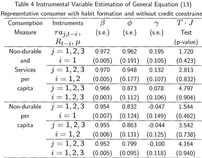
Table 4 Instrumental Variable Estimation of General Equation (13)

Representative consumer with habit formation and without credit constrained

Consumption lnstruments (3

cp

ry T·J

Measure _raj,t-i' (s.e.) (s.e.) (s.e.) Test

Rt-i, p, (p-value)

Non-durable j

= 1,2,3

0.972 0.962 0.195 1.720 and

i= 1

(0.005) (0.191) (0.105) (0.423) Services j

= 1, 2, 3

0.970 0.948 0.132 2.813

per

i- 1 2

_-

_'

(0.005) (0.177) (0.107) (0.832) capita j

= 1,2,3

0.966 0.873 0.078 4.797

i= 1,2,3

(0.003) (0.112) (0.106) (0.904) Non-durable j

= 1,2,3

0.954 0.832 -0.047 1.544

per

i=1

(0.007) (0.124) (0.149) (0.462) capita j

= 1, 2, 3

0.955 0.863 -0.044 3.542

i- 1 2

_-

_'

(0.006) (0.131) (0.125) (0.738)

j

= 1,2,3

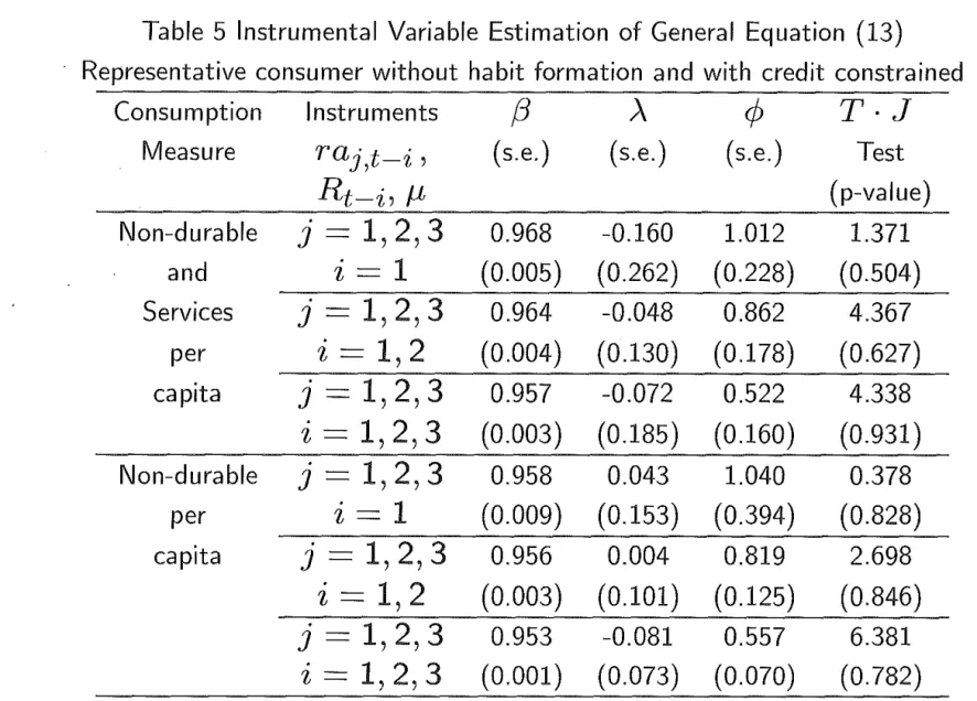
0.952 0.799 -0.100 4.164

Table 5 Instrumental Variable Estimation of General Equation (13)

· Representative consumer without habit formation and with credit constrained

Consumption lnstruments fJ À

cp

T·J

Measure _raj,t-í' (s.e.) ( s.e.) (s.e.) Test

Rt-í, fL (p-value)

Non-durable j = 1,2,3 0.968 -0.160 1.012 1.371

and i= 1 (0.005) (0.262) (0.228) (0.504)

Services j = 1,2,3 0.964 -0.048 0.862 4.367

per i - 1 2 _-

_'

(0.004) (0.130) (0.178) (0.627)

capita j=1,2,3 0.957 -0.072 0.522 4.338

i=1,2,3 (0.003) (0.185) (0.160) (0.931)

Non-durable

j

= 1,2,3 0.958 0.043 1.040 0.378 per i=1 (0.009) (0.153) (0.394) (0.828) capita

j

= 1,2,3 0.956 0.004 0.819 2.698

i -_- 1 2

_'

(0.003) (0.101) (0.125) (0.846)

j

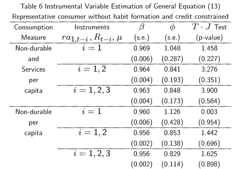
= 1,2,3 0.953 -0.081 0.557 6.381

Table 6 Instrumental Variable Estimation of General Equation (13) Representative consumer without habit formation and credit constrained

Consumption lnstruments (3

_cP

T · J Test Measure _{ra1 t-i , Rt__:_i, /L} (s.e.) (s.e.) (p-value)

Non-durable i= 1 0.969 1.048 1.458

and (0.006) (0.287) (0.227)

Services i= 1, 2 0.964 0.841 3.276

per (0.004) (0.193) (0.351)

capita i=1,2,3 0.963 0.848 3.900

(0.004) (0.173) (0.564)

Non-durable i= 1 0.960 1.126 0.003

per (0.006) (0.428) (0.954)

capita i= 1, 2 0.956 0.853 1.442

(0.002) (0.138) (0.696)

i=1,2,3 0.956 0.829 1.625

llllllllllllllllllll/1 11111

(BIBLIODATA)BB002936753

f I