Estimation of friction parameters in gravity currents by data assimilation in a model hierarchy

(1)

OSD

8, 159–187, 2011

Estimation of friction parameters in gravity

currents by data assimilation

A. Wirth

Title Page

Abstract Introduction

Conclusions References

Tables Figures

◭ ◮

Back Close

Full Screen / Esc

Printer-friendly Version

Interactive Discussion

Discussion

P

a

per

|

Dis

cussion

P

a

per

|

Discussion

P

a

per

|

Discussio

n

P

a

per

|

Ocean Sci. Discuss., 8, 159–187, 2011 www.ocean-sci-discuss.net/8/159/2011/ doi:10.5194/osd-8-159-2011

Ocean Science Discussions

This discussion paper is/has been under review for the journal Ocean Science (OS). Please refer to the corresponding final paper in OS if available.

Estimation of friction parameters in

gravity currents by data assimilation in a

model hierarchy

A. Wirth

LEGI/MEOM/CNRS, France

Received: 11 October 2010 – Accepted: 8 November 2010 – Published: 24 January 2011

Correspondence to: A. Wirth (achim.wirth@hmg.inpg.fr)

(2)

OSD

8, 159–187, 2011

A. Wirth

Title Page

Tables Figures

◭ ◮

Back Close

Full Screen / Esc

Discussion

P

a

per

|

Dis

cussion

P

a

per

|

Discussion

P

a

per

|

Discussio

n

P

a

per

|

Abstract

This paper is the last in a series of three investigating the friction laws and their parametrisation in idealised gravity currents in a rotating frame. Results on the dy-namics of a gravity current (Wirth, 2009) and on the estimation of friction laws by data assimilation (Wirth and Verron, 2008) are combined to estimate the friction

parame-5

ters and discriminate between friction laws in non-hydrostatic numerical simulations of gravity current dynamics, using data assimilation and a reduced gravity shallow water model.

I demonstrate, that friction parameters and laws in gravity currents can be estimated using data assimilation. The results clearly show that friction follows a linear Rayleigh

10

law for small Reynolds numbers and the estimated value agrees well with the analytical value obtained for non-accelerating Ekman layers. A significant and sudden departure towards a quadratic drag law at an Ekman layer based Reynolds number of around 800 is shown, in agreement with classical laboratory experiments. The drag coe_fficient obtained compare well to friction values over smooth surfaces. I show that data

assim-15

ilation can be used to determine friction parameters and discriminate between friction laws and that it is a powerful tool in systematically connection models within a model hierarchy.

1 Introduction

The realism todays and tomorrows numerical models of the ocean dynamics is and

20

will be governed by the accuracy of the parametrisations of the processes not explicitly resolved and resolvable in these models. A typical example is the thermohaline circu-lation of the world ocean, a basin-scale long-time circucircu-lation. It is key to the climate dynamics of our planet and it is governed by small scale processes. The thermohaline circulation starts with the convective descent of dense water masses at high latitudes,

25

(3)

OSD

8, 159–187, 2011

A. Wirth

Title Page

Tables Figures

◭ ◮

Back Close

Full Screen / Esc

Discussion

P

a

per

|

Dis

cussion

P

a

per

|

Discussion

P

a

per

|

Discussio

n

P

a

per

|

a gravity current is created, which is strongly influenced by the friction forces at the ocean floor (Wirth, 2009). The bottom friction is influenced by the dynamics at scales of the order of one meter and less. Similar small scale processes are likely to deter-mine the subsequent deep western boundary current and the upward transport and the mixing in the interior and coastal regions of the ocean. These small scale

pro-5

cesses will not be explicitly resolved in ocean general circulation models (OGCMS) even in a far future. The understanding and parametrisation of these processes is of paramount importance to the progress in modelling the dynamics of the climate.

In the present work I focus on bottom friction determined by small scale three di-mensional turbulence. This process has much smaller spacial scales and faster time

10

scales than the large scale circulation above. This scale separation in space and time is the prerequisite of an efficient parametrisation of bottom friction. Two types of bottom friction laws are commonly employed in engineering and geophysical fluid dynamics applications: a Rayleigh friction with a friction force per unit areaF=ρhτu depending linearly on the fluid speeduat some distance of the boundary and a quadratic drag law

15

F=ρcD|u|u, whereτ andcD are the linear friction parameter and the drag coefficient, respectively,his the thickness of the fluid layer andρthe density of the fluid. In todays ocean general circulation models a mixture of both laws is commonly employed, where the friction force per unit area is given by

F=ρcD p

u2₊_c2_u. ₍₁₎

20

The velocitycrepresents unresolved velocity due to tidal motion and other unresolved short time-scale processes. Typical values forc are a few tenths of centimetres per second. Such friction law leads asymptotically to a linear friction law for small velocities

u≪cand to a quadratic drag law foru≫c.

The precise determination of friction laws and parameters are also fundamental to

25

(4)

OSD

8, 159–187, 2011

A. Wirth

Title Page

Tables Figures

◭ ◮

Back Close

Full Screen / Esc

Discussion

P

a

per

|

Dis

cussion

P

a

per

|

Discussion

P

a

per

|

Discussio

n

P

a

per

|

Bottom friction has also been identified as an important process acting as a sink of kinetic energy. Kinetic energy is principally injected into the ocean by the surface wind-stress at the basin scale. It can only be dissipated at scales where molecular viscosity is acting, that is below the centimetre scale. The pathway of the energy from the basin scale to the dissipation scale is currently to large parts unexplored. The turbulent

5

bottom boundary layer dissipates energy at a rate proportional tocDV 3

wherecDis the (local) drag coefficient and V the (local) flow speed near the boundary. The fact that the energy dissipation is proportional to the third power of the speed emphasises the importance of high speed events and processes in the vicinity of the ocean floor. The determination of the precise value of the drag coefficient which varies over an order

10

of magnitude depending on the roughness of the boundary (see e.g., Stull, 1988) is, therefore, key to determining the energy fluxes and budget of the worlds ocean.

In the present work I focus on the dynamics of oceanic gravity currents which is governed by bottom friction, as it was shown in Wirth (2009). Gravity currents are clearly high-speed events at the ocean floor with speeds of over 1 ms−1. Friction laws

15

and parametrisations at solid boundaries have been a major focus of research in fluid dynamics for the last century, due to their paramount importance in engineering appli-cations. Although large progress has been made in determining the friction over rough boundaries (see e.g., Jim ´enez, 2004) the friction depends of a variety of properties of the ocean floor which are undetermined, as for example: the roughness type, the

20

roughness scales, the multi-scale properties of its roughness, the sediment suspen-sion, the orientation of the roughness elements and the variability of the roughness, to mention only a few. Furthermore, these properties will not be available to ocean mod-ellers in the foreseeable future. In the present work I determine the friction laws and parameters by observing the time evolution of the thickness of a gravity current. In the

25

(5)

OSD

8, 159–187, 2011

A. Wirth

Title Page

Tables Figures

◭ ◮

Back Close

Full Screen / Esc

Discussion

P

a

per

|

Dis

cussion

P

a

per

|

Discussion

P

a

per

|

Discussio

n

P

a

per

|

problem of determining the friction laws and parameters from the evolution of the grav-ity current, I use data assimilation. The formalism of estimating friction laws in oceanic gravity currents has been introduced and discussed in Wirth and Verron (2008). The purpose of the present work is not to use data assimilation so that the shallow water model mimics the non hydrostatic dynamics, but to extract the friction parameters and

5

laws from the hydrostatic dynamics.

I am here interested in the dynamics that governs the thick part of the gravity current, called the vein (see Wirth, 2009). The friction layer, the thin part at the down-slope side of the vein, represents a water mass that is lost for the gravity current, does not contribute to its further evolution, and is mixed into the surrounding water in a short

10

time. The dynamics of the friction layer, which is less than 20 m thick, is also likely to be determined by small scale structures of the ocean floor.

This paper is the last in a series of three. In the first (Wirth and Verron, 2008) we determined the feasibility and convergence of estimating friction parameters while ob-serving only the thickness of the gravity current. In the second (Wirth, 2009), I studied

15

the dynamics of an idealised gravity current using a non-hydrostatic numerical model. I showed that such a gravity current has a two part structure consisting of a vein, the thick part, which is close to a geostrophic dynamics mostly perturbed by the influence of the Ekman pumping caused by bottom friction. At the down-slope side of the vein is the friction layer, the other part, completely governed by frictional dynamics. In the present

20

work the two approaches are combined. The data is taken from non-hydrostatic nu-merical simulations of Wirth (2009) and provided to the assimilation scheme introduced in Wirth and Verron (2008). For the present paper to be self-contained, an overlap to the two previous papers is unavoidable.

The methodology presented here, although developed for the case of idealised

grav-25

(6)

OSD

8, 159–187, 2011

A. Wirth

Title Page

Tables Figures

◭ ◮

Back Close

Full Screen / Esc

Discussion

P

a

per

|

Dis

cussion

P

a

per

|

Discussion

P

a

per

|

Discussio

n

P

a

per

|

laboratory experiments. An example is given by Sun et al. 2002 and Kondrashov et al. 2008 using an extended Kalman filter.

In the next section I introduce the physical problem considered and the two mathe-matical models employed to study its dynamics, followed by a discussion of their nu-merical implementations. The data assimilation algorithm connecting the two models

5

is discussed in Sect. 3. A detailed presentation of the experiments performed is given in Sect. 4, results are presented in Sect. 5 and discussed in Sect. 6.

2 Idealised oceanic gravity current on the f-plane

2.1 The physical problem considered

In the numerical experiments I use an idealised geometry, considering an infinite gravity

10

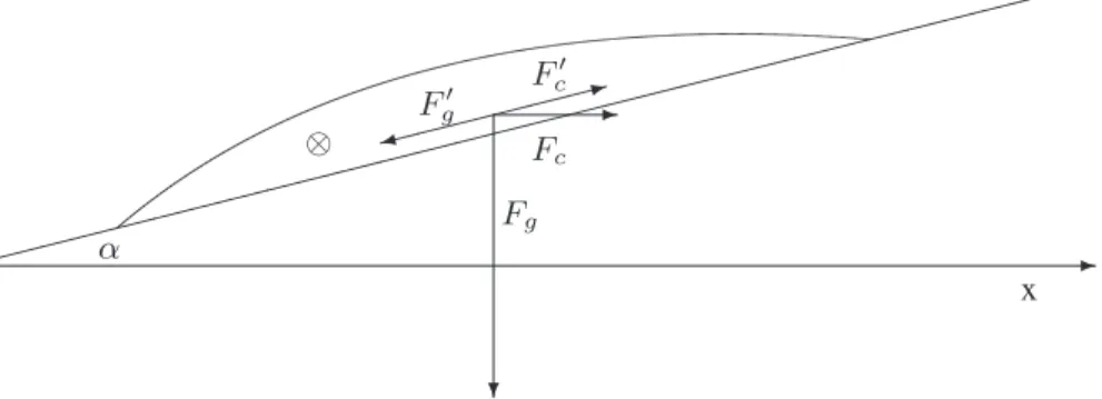
current in a rotating frame on an inclined plane with a constant slope, and I do not allow for variations in the long-stream direction. As discussed in Wirth (2009) a gravity current dominated by rotation is, to leading order, in a geostrophic equilibrium where the downslope acceleration due to gravity is balanced by the Coriolis force. Such gravity current flows along-slope, not changing its depth (see Fig. 1). It is friction that

15

makes a rotating gravity current flow downslope. This is the opposite in non-rotating gravity currents, where friction opposes the downslope movement and results from studies of non-rotating gravity currents can not be applied to rotating gravity currents. In the geometry considered here, I neglect the long-stream variation of the gravity current. Such a dynamics is usually referred to as 2.5-D as it includes the fully three

20

dimensional velocity vector but depends on only two space dimensions. Please note, that such simplified geometry inhibits large scale instability, the formation of the large cyclones and other large-scale features, which is beneficial to our goal of studying the friction laws due to only small scale dynamics.

The initial condition is a temperature anomaly which has a parabolic shape which

25

(7)

OSD

8, 159–187, 2011

A. Wirth

Title Page

Tables Figures

◭ ◮

Back Close

Full Screen / Esc

Discussion

P

a

per

|

Dis

cussion

P

a

per

|

Discussion

P

a

per

|

Discussio

n

P

a

per

|

The physical problem is considered with the help of two mathematical models of di_fferent complexity. The first are the Navier-Stokes equations with a no-slip boundary condition on the ocean floor, subject to the Boussinesq approximation. The second is a single layer reduced gravity shallow water model. The bottom friction is explicitly resolved in the first while it has to be parametrised in the second.

5

2.2 The Navier-Stokes model

The mathematical model for the gravity current dynamics are the Navier-Stokes equa-tions subject to the Boussinesq approximation in a rotating frame with a buoyant scalar (temperature). The state vector is formed by the temperature anomaly of the gravity current water with respect to the surrounding water and all the three components of

10

the velocity vector. I neglect variations in the stream wise (y-) direction of all the vari-ables. Such type of model is usually referred to as 2.5-D. The x-direction is upslope (see Fig. 1). This leads to a four dimensional state vector depending on two space and the time variable, (∆T(x,z,t),u(x,z,t),v(x,z,t),w(x,z,t)).

The domain is a rectangular box that spans 51.2 km in thex-direction and is 492 m

15

deep (z-direction). On the bottom there is a no-slip and on the top a free-slip boundary condition. The horizontal boundary conditions are periodic. The initial condition is a temperature anomaly which has a parabolic shape which is 200 m high and 20 km large at the bottom, as described in the previous subsection. The magnitude of the temperature anomaly∆T is varied between the experiments. The reduced gravity is

20

g′=g·2_×10−4K−1_·_∆T withg=9.8066 ms−2. The Coriolis parameter isf=1.03_×10−4s−1. The initial velocities in the gravity current are geostrophically adjusted:

u_G=0;v_G=g

′₍_∂

xh+tanα)

f ;wG=0. (2)

the fluid outside the gravity current is initially at rest. The buoyancy force is represented by an acceleration of strength g′cos(α) in the z-direction and g′sin(α) in the

nega-25

(8)

OSD

8, 159–187, 2011

A. Wirth

Title Page

Tables Figures

◭ ◮

Back Close

Full Screen / Esc

Discussion

P

a

per

|

Dis

cussion

P

a

per

|

Discussion

P

a

per

|

Discussio

n

P

a

per

|

a rectangular box that is tilted by an angle of one degree. Such implementation of a sloping bottom simplifies the numerical implementation and allows for using powerful numerical methods (see next subsection).

2.3 Numerical implementation of the Navier-Stokes model

The numerical model used is HAROMOD (Wirth, 2004). HAROMOD is a pseudo

5

spectral code, based on Fourier series in all the spatial dimensions, that solves the Navier-Stokes equations subject to the Boussinesq approximation, a no-slip boundary condition on the floor and a free-slip boundary condition at the rigid surface. The time stepping is a third-order low-storage Runge-Kutta scheme. A major difficulty in the nu-merical solution is due to the large anisotropy in the dynamics and the domain, which is

10

roughly 100 times larger than deep. There are 896 points in the vertical direction. For a density anomaly larger than 0.75 K the horizontal resolution had to be increased from 512 to 2048 points (see Table 1), to avoid a pile up of small scale energy caused by an insufficient viscous dissipation range, leading to a thermalized dynamics at small scales as explained by Frisch et al. (2008). The horizontal viscosity isνh=5 m

2

s−1, the

hor-15

izontal diffusivity isκh=1 m 2

s−1. The vertical viscosity is νv=10− 3

m2s−1, the vertical diffusivity isκv=10−

4

m2s−1. The anisotropy in the turbulent mixing coefficients reflects the strong anisotropy of the numerical grid. I checked that the results presented here show only a slight dependence onνh,κhandκvby doubling these constants in a control run. This is no surprise as the corresponding diffusion and friction times are larger than

20

the integration time of the experiments. There is a strong dependence onν_v as it de-termines the thickness of the Ekman layer and the Ekman transport, which governs the dynamics of the gravity current as I have shown in Wirth (2009). The vertical extension of the Ekman layer is a few meters while the horizontal extension of the gravity current is up to fifty kilometres. In a fully turbulent gravity current the turbulent structures within

25

(9)

OSD

8, 159–187, 2011

A. Wirth

Title Page

Tables Figures

◭ ◮

Back Close

Full Screen / Esc

Discussion

P

a

per

|

Dis

cussion

P

a

per

|

Discussion

P

a

per

|

Discussio

n

P

a

per

|

necessary in the horizontal direction to obtain an isotropic grid. This is far beyond our actual computer resources.

The time of integration is limited due to the descending gravity current leaving the domain of integration when sliding down the slope, which depends on the initial density anomaly. The actual integration times in all experiments are given in Table 1.

5

2.4 The shallow water model

The second, and less involved, mathematical model for the gravity current dynamics is a 1.5-D reduced gravity (1.5 layer) shallow water model on an inclined plane. The shallow water model, first proposed by Barr ´e de Saint Venant (1871), and its various versions adapted for specific applications is one of the most widely used models in

10

environmental and industrial fluid dynamics. For the derivation of the reduced gravity shallow water equations in a geophysical context, I refer the reader to the text book by Vallis (2006), and references therein.

As stated in the introduction I here specialise to a gravity current with no variation in they-direction, the horizontal direction perpendicular to the down-slope direction.

15

That is I have three scalar fields ˜u(x,t), ˜v(x,t) and h(x,t) as a function of the two scalars x and t. The thickness of the gravity current is given by h. The velocities

˜

u(x,t)₌Rh

0u(x,z,t)d z/h and ˜v(x,t)= Rh

0v(x,z,t)d z/h represent the vertical averages over the whole layer thickness h(x,t) of the local velocity components u(x,z,t) and

v(x,z,t). I further suppose that the dynamics within the gravity current is well

de-20

scribed by a two-layer structure: an Ekman layer with a thickness scaleδ=

q

2ν_v/f at the bottom and the rest of the gravity current above. To take into account several fea-tures of the gravity current dynamics discovered with the non-hydrostatic model (see Wirth, 2009), the shallow-water model employed in Wirth and Verron (2008) had to be refined. Results presented in Wirth (2009) show, in agreement with Ekman layer

25

(10)

OSD

8, 159–187, 2011

A. Wirth

Title Page

Tables Figures

◭ ◮

Back Close

Full Screen / Esc

Discussion

P

a

per

|

Dis

cussion

P

a

per

|

Discussion

P

a

per

|

Discussio

n

P

a

per

|

the Coriolis-Boussinesq variable:

β=h

Rh 0u

2

d z

(R₀hud z)2>1 (3)

If there is no vertical shearβ=1. If there is no bottom friction, the shear in a homoge-neous fluid layer is small andβ≈1. When Ekman layers are present there is substantial shear andβ>1. Ekman layers are a conspicuous feature in all geophysical flows

sub-5

ject to bottom friction and this has to reflected in the mathematical model employed. In a shallow water model this can be done by explicitly via the Coriolis-Boussinesq variable. The Coriolis-Boussinesq variable is a function of the variation of the veloc-ity profile in the vertical. When using the linear Ekman spiral, I obtain to first order

β=h/(2δ) when h≫δ which depends on the layer thicknessh and is thus a function

10

of space and time. Please see the Appendix A for details concerning the calculations of the Coriolis-Boussinesq variable. The Coriolis-Boussinesq variable is widely used in mathematical modelling of river dynamics and appears naturally when the shallow-water equations are systematically derived for flow with vertical shear of the horizontal velocities (see Gerbeau and Perthame, 2001).

15

The governing equations for the velocities vertically averaged over the whole thick-ness of the dynamic layerh, Ekman layer plus the rest above, are given by:

∂_tu˜+βu∂˜ _xu˜₋fv˜+g′(∂_xh+tanα)=−D_uu˜+ν∂_x2u,˜ (4)

∂_tv˜+fu˜=−D_vv˜+ν∂2

xv,˜ (5)

20

∂th+u∂˜ xh+h∂xu˜=ν∂x2h. (6)

(11)

OSD

8, 159–187, 2011

A. Wirth

Title Page

Tables Figures

◭ ◮

Back Close

Full Screen / Esc

Discussion

P

a

per

|

Dis

cussion

P

a

per

|

Discussion

P

a

per

|

Discussio

n

P

a

per

|

theuvelocity is concentrated in the Ekman layer and

hRh 0uv d z (Rh

0ud z)( Rh

0v d z)

<1. (7)

On the right hand side I have the terms involving dissipative processes. Please note that this includes the bottom friction as well as the friction at the interface, in numeri-cal experiments with the non-hydrostatic model (Wirth, 2009) the latter is found to be

5

smaller than the former. The parametrised friction is represented in the first term on the left hand side, involving:

Du=Du(x,t)=4β

τ+r/h2+cD q

(4βu˜)2₊_v_˜2

/h. (8)

Dv=Dv(x,t)=

τ+r/h2+cD q

(4βu˜)2₊_v_˜2

/h. (9)

The Coriolis-Boussinesq variableβin Eq. (8) is explained in the Appendix. There are

10

three free parametersτ,r andcD. There is a linear friction constant parametrising dis-sipative effects that can be represented by linear Rayleigh friction. This linear friction is represented by two parametersτandr, the first represents the part that is independent of the thickness and the second is divided by the square of the thickness. Usually the thickness of laminar boundary layers grows in time, when the dynamics is influenced

15

by rotation, this growth is halted creating the well known Ekman layer dynamics (see e.g., Vallis, 2006). Using only the term containing the parameterτ represents well the dynamics when an Ekman layer is developed, that is, when the thickness of the gravity current is larger than a few times the Ekman layer thickness. For smaller thicknesses, smaller than a few times the Ekman-layer thickness, a term involving the thickness of

20

(12)

OSD

8, 159–187, 2011

A. Wirth

Title Page

Tables Figures

◭ ◮

Back Close

Full Screen / Esc

Discussion

P

a

per

|

Dis

cussion

P

a

per

|

Discussion

P

a

per

|

Discussio

n

P

a

per

|

interested in the friction forces acting on the vein as stated in the introduction. In the re-sults presented below the friction force due to the depth dependent term is a negligible part of the total friction, in the vein. The quadratic friction dragcD, models the turbulent friction between the ground and the gravity current. The Coriolis-Boussinesq variable is given byβ=h/(2δ) for large values of the layer thickness, as derived in Appendix A.

5

Ifβis smaller than 2 it is put equal to 2 in the advection term and if it is smaller than 1/4 it is put to 1/4 in the friction terms. The first choice is consistent with the fact that in the advection term the Coriolis-Boussinesq variable is by definition always larger than unity. Concerning the friction terms: for large layer thickness,βagrees with the value calculated in the Appendix A and for a very small layer thickness,β=1/4 agrees with

10

the fact that the friction in thex and y direction in Eqs. (8) and (9) should have the same form in the absence of an Ekman spiral. I checked that the choices for these thresholds have only a negligible influence on the results. The term involving the vis-cosity/di_ffusivity ν represents horizontal dissipative processes, its value is chosen to provide numerical stability of the calculations (see Sect. 2.5).

15

Clearly, the geostrophic velocity 2:

is a solution of Eqs. (4–6) when Du=Dv=0 and ν=0. The estimation of D or more

precisely of the parametersτ,r and cDare the subject of the present work. By using data assimilation I plan to obtain the friction constantsτ andcDand thus determine if the friction acting on the vein is dominated by a linear or a quadratic law.

20

2.5 Numerical implementation of the shallow water model

The shallow water model is implemented with a first order finite difference scheme in space and time. There are 500 points in the x-direction, leading to a resolution of 200 m, the time step is 5 s. The value of the horizontal viscosity/diffusivity is a func-tion of the resolufunc-tion and provides for the numerical stability of the code. I verified

25

that the here presented results show only a negligible dependence when the value of the horizontal viscosity/diffusivity was halved and doubled, the actual value used is

(13)

OSD

8, 159–187, 2011

A. Wirth

Title Page

Tables Figures

◭ ◮

Back Close

Full Screen / Esc

Discussion

P

a

per

|

Dis

cussion

P

a

per

|

Discussion

P

a

per

|

Discussio

n

P

a

per

|

3 Ensemble Kalman filter and its implementation

For this publication to be self contained, the implementation of the Ensemble Kalman filter is explained here, the reader familiar with Wirth and Verron (2008) is invited to skip the section. Further details about the data assimilation procedure and the convergence properties are explained in (Wirth and Verron, 2008).

5

The ensemble Kalman filter (EnKF) is the main tool of our experiments performing the parameter estimation and providing us with the actual parameter values. The EnKF was introduced by Evensen (1994) and is used in data assimilation and parameter estimation experiments (see Evensen, 2003; Brusdal et al., 2003). I refer the reader not familiar with the EnKF and the employed notation to the above mentioned publications.

10

Every hour in time and every 1 km in the x-direction, the vertical extension of the gravity current, that ish(x,t), is assimilated. Choosing a horizontal resolution for the assimilation 5 times sparser than the dynamical model does not only reduce the size of the assimilation experiment, but is also consistent with the fact, that the grid-scale dynamics of the numerical model is dominated by dissipation and has only

negligi-15

ble dynamical information. I am only assimilating the vertical extension of the gravity current as it is the variable most easily measured in the ocean and in laboratory experi-ments. The measurement of the vertically integrated velocity within the gravity current, the other dynamical variable of the shallow water model, is more difficult to measure in the ocean and in laboratory experiments.

20

The assimilation is performed on the augmented state vector consisting of the verti-cal extension, the two velocity components and the three constant-in-time friction pa-rameters:

x( ¯x,_t¯₎₌ _h_{( ¯}_x,_t¯₎_,u˜( ¯x,_t¯₎_,v˜( ¯x,_t¯₎_,τ,r,c_Dt_. ₍₁₀₎ Where ¯x and ¯t is the discretized version of x at assimilation grid-points andt at

as-25

(14)

OSD

8, 159–187, 2011

A. Wirth

Title Page

Tables Figures

◭ ◮

Back Close

Full Screen / Esc

Discussion

P

a

per

|

Dis

cussion

P

a

per

|

Discussion

P

a

per

|

Discussio

n

P

a

per

|

EnKF reads,

xa

i =x f i+K

hobs

+ǫ_i₋Hxf

i

(11)

K=PHt(HPHt+R)−1 (12)

Where the index i=1,...,m runs over the realisations. The observation operator H 5

projects the state vector in the space of observations. The noise vectors ǫ_i repre-sents the independent Gaussian-distributed zero-mean andσ-standard-deviation noise added to every observed value (see Burgers et al., 1998) andW=σ2I whereI is the unity matrix. The estimated error covariance matrix is given by

P= 1

m−1

m

X

i=1

xf

i−hx f

i xf

i −hx f

it, (13)

10

wheremis the size of the ensemble and_h._idenotes an ensemble average. The covari-ance matrix is truncated to a tridiagonal form to avoid spurious correlations between distant correlations, caused by under sampling. This is also consistent with the dy-namics at hand as the maximum velocities (see Sect. 2.1) and wave speeds, given by p

g′_h _{are of the order of 0}_._{2 ms}−1_{. This means that in the assimilation period of 1 h} 15

information can travel to the next assimilation point one kilometre away, but it can not reach over the distance of two assimilation grid points. In between assimilation points

his interpolated linearly.

In general the observed value of the vertical extension of the gravity current

hobs(x,t) includes measurement errors η(x,t) and is related to the true value by

20

hobs(x,t)=htrue(x,t)+η(x,t). For consistency the measurement error η(x,t) has the same first (zero mean) and second order moment ( ˜σ2) as the noise vectorsǫ_i(x,t), but does not depend on the actual realisation, that isi. When assimilating data,σ has to be provided prior to the experiment whereas ˜σ is usually not known and can only be estimated.

(15)

OSD

8, 159–187, 2011

A. Wirth

Title Page

Tables Figures

◭ ◮

Back Close

Full Screen / Esc

Discussion

P

a

per

|

Dis

cussion

P

a

per

|

Discussion

P

a

per

|

Discussio

n

P

a

per

|

In our parameter estimation experiments, the ensemble size ism=100, this is much larger than the number of parameters to estimate, that is three, equal to the number of observations at each assimilation time, but smaller than the dimension of the aug-mented state vectorx₌(h,u,˜ v˜,τ,r,cD), that is 303. Using an ensemble size an order of magnitude larger did not improve the convergence significantly, reducing the ensemble

5

size an order of magnitude leads to a frequent divergence of the assimilation.

It is important to note that not only the parameter values are estimated, but the entire state vector is updated every time data is assimilated. This allows to perform parameter estimation in the case where the shallow-water model is unable, even with perfectly adjusted parameters, to reproduce some aspects of the Navier-Stokes

dy-10

namics. Entrainment is a typical example, it happens in the Navier-Stokes dynamics, there is no reliable parametrisation available for the shallow-water model and friction parameters can not account for all the impacts of entrainment on the evolution of the layer-thickness. Trying to estimate the friction parameters without correcting the other values of the state vector frequently leads to a divergence of the estimation procedure

15

in experiments where mixing, entrainment or detrainment is present (experiments with high values of the density anomaly).

Another important point is, that the parameter values are supposed to be constant in time. The values of the friction parameters are clearly non-negative, so every time the assimilation scheme provides a negative value of one of these parameters, which is

20

possible due to the linearity of the analysis step and the statistical nature of the EnKF, the value is put to zero.

All pseudo-random-numbers were generated by a “Mersenne Twister” (Matsumoto and Nishimura, 1998).

4 Experiments 25

(16)

OSD

8, 159–187, 2011

A. Wirth

Title Page

Tables Figures

◭ ◮

Back Close

Full Screen / Esc

Discussion

P

a

per

|

Dis

cussion

P

a

per

|

Discussion

P

a

per

|

Discussio

n

P

a

per

|

vertical extension, that is the density structure of a gravity current is the variable that is easiest to measure and to observe in the ocean and in laboratory experiments. Ve-locities, even their average values are hard to determine as they are highly variable in space and intermittent in time. The thickness h is extracted from the runs of the Navier-Stokes model, it is determined by the position above ground of the thermocline

5

that corresponds to half the initial maximum temperature anomaly in the gravity current at the assimilation pointsx, every 1 km, and the assimilation timest, every hour. It is the time series of these shapesh(x,t), and only these, which are provided to the as-similation run to determine the friction parameters. Please note that the space integral ofh, the total volume, is not conserved but has some slight variation due to mixing,

10

entrainment and detrainment, whereas in the shallow water model without assimilation it is conserved. The data assimilation procedure corrects the total state vector, includ-ing theh-value and the method can thus deal consistently with variations in the total gravity current fluid volume (or area in our 2.5-D case).

The important results concerning the data assimilation experiments, as for example:

15

convergence properties of the friction parameters and a good choice of the observation frequency and other parameters are discussed in (Wirth and Verron, 2008).

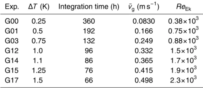
A series of seven experiments was performed. The density anomaly∆T is the only parameter varied between the experiments. A list of all experiment performed, the du-ration of the experiment, the average geostrophic velocity ¯vgand the Reynolds number,

20

ReEk=

vgδ

ν_v =

∆T·2_×10−4K−1gtan(α)√2

√

f3_ν = ∆T·1.5×10 3

K−1, (14)

based on the Ekman layer thickness, given byδ=

q

2ν/f, are shown in Table 1. The Reynolds number based on the Ekman layer thickness, is the determining parame-ter for laminar flow. When vertical velocities develop (absent in the homogeneous linear Ekman layer), the now turbulent Ekman layer increases in thickness and the

25

(17)

OSD

8, 159–187, 2011

A. Wirth

Title Page

Tables Figures

◭ ◮

Back Close

Full Screen / Esc

Discussion

P

a

per

|

Dis

cussion

P

a

per

|

Discussion

P

a

per

|

Discussio

n

P

a

per

|

temperature anomalies of about one Kelvin. When vertical velocities are important the flow is characterised by the surface Rossby number,

Ro= vg

f z0

=vgu∗

f ν_v =

√_c

Dv 2 g

f ν_v , (15)

wherez0is the roughness length, which for smooth surfaces is given byz0=νv/u∗. The

friction velocityu_∗=√cDvgand the surface Rossby number are results of our numerical

5

calculations, rather than an initial parameter, and is therefore presented in Table 2 of the results section. In the turbulent boundary layer vertical velocities of orderu_∗ de-velop. The typical length scale is now formed by a balance between rotation e_ffects and vertical velocityδturb≈u_∗/f, rather than the balance between viscosity and rotation for the laminar case. Observations show that the actual thickness of the turbulent Ekman

10

layer is_≈δturb/4, including a log-layer of thickness≈δturb/10. The above teaches us, that the surface Rossby number is the equivalent to the Ekman-scale Reynolds number with a turbulent Ekman layer thicknessδturb replacing the laminar Ekman layer thick-nessδ. The former characterises turbulent flow and the latter laminar flow. To avoid confusion I continue to discriminate between the experiments in terms of temperature

15

anomaly rather than Reynolds or surface Rossby number. The surface Rossby number is also a measure of the thickness of the turbulent Ekman layer (or the log-layer) to the thickness of the viscous sub-layerδsub=ν/u_∗ (please see McWilliams, 2006, chapter 6 for a concise introduction to planetary boundary layer dynamics). I refer the reader to Wirth (2009) for a more detailed description of the gravity current dynamics considered

20

here.

In the data assimilation experiment the observation error for the layer thickness was set to σ=10 m. I checked that the results presented in the next section do not de-pend significantly on the actual value ofσ when chosen within reasonable limits. The assimilation is done every hour, the length of the experiment is given in Table 1 and

as-25

(18)

OSD

8, 159–187, 2011

A. Wirth

Title Page

Tables Figures

◭ ◮

Back Close

Full Screen / Esc

Discussion

P

a

per

|

Dis

cussion

P

a

per

|

Discussion

P

a

per

|

Discussio

n

P

a

per

|

for the parameters was chosen randomly, with an ensemble mean value at the order of magnitude of the expected values. The procedure was iterated by using the ensem-ble at the end of a assimilation experiment as the initial ensemensem-ble for the consecutive experiment. I also tried inflation of the ensemble values, the distance from the en-semble mean was increased by a constant factor for every enen-semble member at every

5

assimilation time, to avoid spurious decrease of the ensemble variance. Inflation did not change significantly the results. All results reported here were done without infla-tion. For further information concerning the assimilation scheme, its performance and convergence properties I like to refer the reader to Wirth and Verron (2008).

The non-hydrostatic calculations were done on 16 parallel processors at IDRIS high

10

performance computation centre, whereas the assimilation of the data by the shallow water model where performed on a lap-top computer. (please see Wirth, 2009; Wirth and Verron, 2008 for further details.)

5 Results

In the case of a (linear stationary) Ekman dynamics, the linear Rayleigh friction can be

15

calculated analytically, as already explained in Wirth (2009):

τ=ν

δ=

r

νf

2 (16)

with an Ekman layer thickness δ=

q

2ν/f. The value for the calculations presented here is:τ=2.27_×10−4ms−1.

I started by performing parameter estimation experiments using the shallow water

20

(19)

OSD

8, 159–187, 2011

A. Wirth

Title Page

Tables Figures

◭ ◮

Back Close

Full Screen / Esc

Discussion

P

a

per

|

Dis

cussion

P

a

per

|

Discussion

P

a

per

|

Discussio

n

P

a

per

|

assimilation) with the estimated values ofτandcDshowed results that compare poorly with the data for the thicknesshfrom the non-hydrostatic calculations in friction layer, where the thickness is small. This problem improved when the parameter space was augmented by the thickness dependent parameterr. In the words of data assimilation: without the calculated Coriolis-Boussinesq variable and the estimated friction

param-5

eterr the assimilation converged to a (local) minimum of the cost function which has a value that is not small enough. In the words of a dynamicist: without the Coriolis-Boussinesq variable and the parameterr an important physical process is missing and the dynamics can not be understood without it. I like to emphasise that without using data assimilation one might have thought that one just did not find the right minimum in

10

parameter space, with data assimilation one can be more confident, so not certain, that the minimum was found but the model had major deficiencies so that it is not capable to represent well enough the dynamics. Anyhow, adding the Coriolis-Boussinesq variable and the thickness dependent friction leads to an improvement of the representation of the dynamics, especially for the cases with a high temperature anomaly (∆T).

15

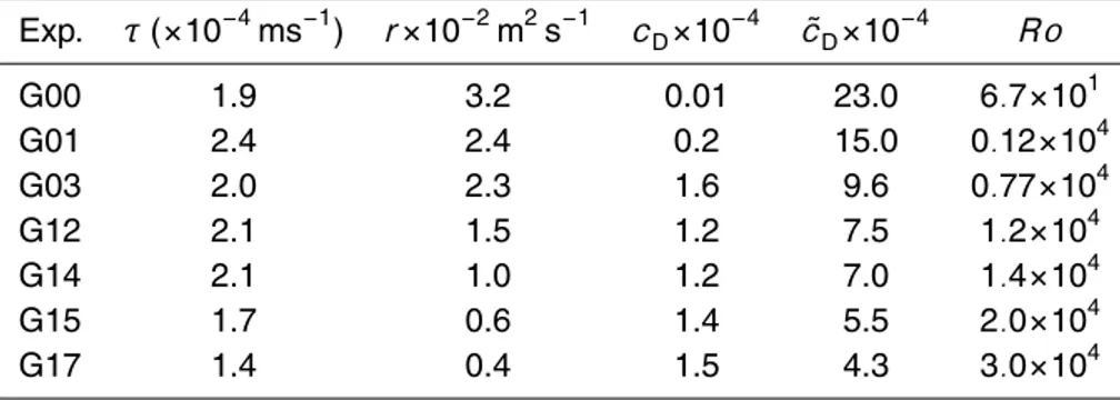
The experiments are listed in Table 1 and results are presented in Table 2. The results for the Rayleigh friction parameter (τ) compare well to the analytical value of Eq. (16) for small values of the temperature anomaly. The impact of the thickness dependent friction parameterr is negligible in the thick part of the gravity current in all the experiments performed (see Table 2). The drag coefficient is small in these cases

20

with a small temperature anomaly but increases abruptly with the temperature anomaly and represents a substantial part of the total friction in the experiments with a larger temperature anomaly. I also calculated for all experiments an effective drag coefficient:

˜

cD=cD+

τ

¯

vg

, (17)

and the surface Rossby number Ro. It is the effective drag coefficient that is

usu-25

(20)

OSD

8, 159–187, 2011

A. Wirth

Title Page

Tables Figures

◭ ◮

Back Close

Full Screen / Esc

Discussion

P

a

per

|

Dis

cussion

P

a

per

|

Discussion

P

a

per

|

Discussio

n

P

a

per

|

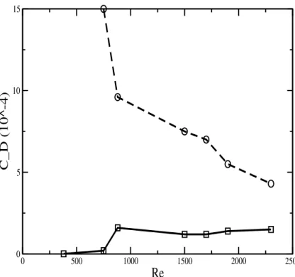
The sudden appearance of a drag law at Reynolds numbersRe_Ek_≈₈_×₁₀2_{is shown.}

The values of the effective drag coefficient are shown in Fig. 2. Another interesting feature of the assimilation procedure is, that I not only obtain e_ffective drag coe_fficient as is usually the case but I clearly manage to separate the friction process in a linear and a quadratic part, gaining further insight in the dynamics.

5

When comparing the dynamics of a free run of the shallow-water model, without data assimilation to the dynamics of the Navier-Stokes model, the agreement is gen-erally satisfactory, but deteriorates with increasing temperature anomaly of the gravity current. I have to emphasise that a di_fference between a free run with adjusted param-eters to the data, does not a priori devaluate the parameter estimation. The difference

10

might originate from a process not represented, neither directly nor parametrised, in the shallow-water model. During the data assimilation this di_fference is corrected by the update of the whole state vector, in the free run this correction is absent. More precisely: entrainment, detrainment and mixing changes the layer thicknesshand the overall volume of the gravity current, the importance of these processes increase with

15

the Reynolds number. The corresponding parameters are not estimated in the shallow-water model. A change of the total volume can not be obtained by changing the friction parameters, as they do not affect the volume of the gravity current. The layer thickness is corrected at every data assimilation as it is part of the state vector. The free run and the data do therefore not necessarily agree, even when the total volume of the gravity

20

current is considered.

As stated in Sect. 3 I supposed the parameters to be constant, a variability in time is clearly detected in all three parameters. Their variability is however small compared to their absolute value.

6 Discussion 25

(21)

OSD

8, 159–187, 2011

A. Wirth

Title Page

Tables Figures

◭ ◮

Back Close

Full Screen / Esc

Discussion

P

a

per

|

Dis

cussion

P

a

per

|

Discussion

P

a

per

|

Discussio

n

P

a

per

|

Rayleigh law for small Reynolds numbers and the estimated friction coefficient agrees well with the analytical value obtained for non-accelerating Ekman layers. A significant and sudden departure towards a quadratic drag law at Reynolds number of around 800 is shown, roughly in agreement with laboratory experiments (Nikuradse, 1933; Schlichting and Gertsen, 2000). It is the e_ffective drag coe_fficient that is usually

repre-5

sented in diagrams like Fig. 2 (dashed line) by the engineering community (Schlichting and Gertsen, 2000). Indeed, when friction processes are considered experimentally, numerically or analytically the results can all be condensed in to a friction force as a function of the Reynolds or surface Rossby number. The graphs and values are than compared in the different experiments and theories. Their overall behaviour consists

10

always in a linear friction law for laminar flow (small Reynolds numbers) and a drag law (large Reynolds numbers) with a roughly constant drag coefficient for turbulent bound-ary layers. For intermediate Reynolds numbers it is difficult to separate the two friction laws without using data assimilation. Although the quadratic drag law is dominated by the linear friction at the Reynolds numbers considered in this study, the

assimila-15

tion procedure clearly manages to detect its appearance and consistently estimate its value. This is of paramount importance when it comes to comparing numerical simu-lations to observations. In the former, the Reynolds numbers typical for the latter are not attainable. The present method allows to extract the value of the quadratic drag co-efficient from simulations at Reynolds numbers where it is largely dominated by linear

20

friction. An extrapolation to the drag at much higher Reynolds number is then possible. The drag coefficient obtained_≈1.5_×10−4 (see Table 2) is on the lower end of clas-sical values over smooth surfaces (see Stull, 1988; Schlichting and Gertsen, 2000). The spectral method used (Wirth, 2004) imposes a smoothness of the surface up to the machine precision (10−16m). This comes at no surprise as only part of the

tur-25

(22)

OSD

8, 159–187, 2011

A. Wirth

Title Page

Tables Figures

◭ ◮

Back Close

Full Screen / Esc

Discussion

P

a

per

|

Dis

cussion

P

a

per

|

Discussion

P

a

per

|

Discussio

n

P

a

per

|

gravity current, but with an isotropic grid resolving the essential turbulent motion, give an increased friction coefficient (preliminary results).

The experiments were performed for moderate surface Rossby numbers as: (i) the numerical resolution in the Navier-Stokes model does not allow for an explicit represen-tation of the fully turbulent Ekman layer (see Sect. 2.3) and (ii) with increasing Rossby

5

number non-hydrostatic effects become important, neither explicitly resolved nor im-plicitly included (parametrised) in the shallow water model used for the assimilation.

Comparison of free runs of the shallow-water model with the estimated parameter values clearly show that the shallow-water model performs well in the vein, whereas it deteriorates in the friction layer with increasing temperature anomaly. In these

ar-10

eas the local Froud number is larger than unity and the oscillations of the interface and its breaking starts to develop. These non-hydrostatic processes are neither explic-itly included in the (hydrostatic) shallow-water model nor are they parametrised. The parametrisation of the dynamics at the interface, including the mixing, entrainment and detrainment, is subject to current research, using higher resolution three dimensional

15

non-hydrostatic simulations of only a small part of the gravity current. Furthermore, to represent the bottom friction in the shallow water model I supposed that unaccelerated linear Ekman layer theory applies to leading order. This assumption is questionable when non-linear effects, leading to a drag law, become dominant.

I demonstrated that the linear dynamics and the nonlinear departure from it are well

20

captured in the present work. I also showed that data assimilation is a powerful tool in systematically connection models in a model hierarchy.

The parameters of the two most observed and employed friction laws, Rayleigh fric-tion and the drag law, are estimated here. The methodology is not restricted to this two laws, this linear and quadratic laws can also be seen, pragmatically, as the beginning

25

of a Taylor series.

(23)

OSD

8, 159–187, 2011

A. Wirth

Title Page

Tables Figures

◭ ◮

Back Close

Full Screen / Esc

Discussion

P

a

per

|

Dis

cussion

P

a

per

|

Discussion

P

a

per

|

Discussio

n

P

a

per

|

currents on the Coriolis platform in Grenoble (France) and measured its thickness. The quantity of data measured was not sufficient to determine the friction parameters and laws. Further laboratory experiments with a substantially increased number of obser-vations are planed.

Appendix A 5

Calculation of the Coriolis-Boussinesq variable for linear Ekman layers

The Solution for the Ekman spiral of a fluid moving with a constant geostrophic speed ofVGin they-direction is given by:

˜

u=VGexp(−z/δ)sin(z/δ) (A1)

10

˜

v=VG 1−exp(−z/δ)cos(z/δ)

, (A2)

where I have denoted ˜uthe variable that has a dependence in thez-direction as op-posed to vertically averaged valueu=hu˜_i=1_hRh0ud z˜ . The vertical average of the velocity component in thex-direction and its square, using Eq. (A1), are:

15

u=hu˜_i=1

h

Zh

0 ˜

ud z=VG

h

Zh

0

exp(₋z/δ)sin(z/δ)d z=VGδ

2h = VG

4β (A3)

u26=hu˜2i=V

2 G

h

Zh

0

exp(₋2z/δ)sin2(z/δ)d zV

2 Gδ 8h =

V_G2

16β. (A4)

Furthermore:

β=hu˜

2

i hu˜_i2=

h

2δ. (A5)

(24)

OSD

8, 159–187, 2011

A. Wirth

Title Page

Tables Figures

◭ ◮

Back Close

Full Screen / Esc

Discussion

P

a

per

|

Dis

cussion

P

a

per

|

Discussion

P

a

per

|

Discussio

n

P

a

per

|

Please note that Eq. (A3) shows that the mean velocity in thex-component is only one quarter of geostrophic velocity divided byβ. Linear Ekman layer theory shows, that the frictional force is equal in both directions, so that in the friction term the u value has to be multiplied by 4β. The non-linear term in the v-equation isu∂_xv is vanishing to leading order ofβ−1as theu-velocity is concentrated in the Ekman layer, whereas the

5

bulk of thev-momentum is above it. I used:

Z

exp(₋z/δ)sin(z/δ)d z=−δ

2 (sin(z/δ)+cos(z/δ)) and (A6)

Z

exp(−2z/δ)sin2(z/δ)d z=−exp(−2z/δ)

8 (2sin 2

(z/δ)+sin(z/δ)cos(z/δ)+1). (A7)

10

I emphasise that these calculations are only valid for the unaccelerated laminar Ekman layer.

References

Brusdal, K., Brankart, J. M., Halberstadt, G., Evensen, G., Brasseur, P., van Leeuwen, P. J., Dombrowsky, E., and Verron, J.: A demonstration of ensemble-based assimilation methods

15

with a layered OGCM from the perspective of operational ocean forecasting systems, J. Mar. Syst., 40–41, 253–289, 2003.

Burgers, G., van Leeuwen, P., and Evensen, G.: Analysis scheme in the ensemble Kalman filter, Mon. Weather Rev., 126, 1719–1724, 1998.

Evensen, G.: Sequential data assimilation with a nonlinear quasi-geostrophic model using

20

Monte Carlo methods to forecast error statistics, J. Geophys. Res., 99, 10143–10162, 1994. Evensen, G.: The ensemble Kalman filter: theoretical formulation and practical implementation,

Ocean Dynam., 53, 343–367, 2003.

Frisch, U., Kurien, S., Pandit, R., Pauls, W., Sankar Ray, S., Wirth, A., and Zhu, J.-Z.: Hyper-viscosity, galerkin truncation, and bottlenecks in turbulence, Phys. Rev. Lett., 101, 144501,

25

(25)

OSD

8, 159–187, 2011

A. Wirth

Title Page

Tables Figures

◭ ◮

Back Close

Full Screen / Esc

Discussion

P

a

per

|

Dis

cussion

P

a

per

|

Discussion

P

a

per

|

Discussio

n

P

a

per

|

Gerbeau, J.-F. and Perthame, B.: Derivation of viscous Saint-Venant system for laminar shallow water; numerical validation, Discrete Cont. Dyn.-B, 1, 89–102, 2001.

Grianik, N., Held, I. M., Smith, K. S., and Vallis, G. K.: The effects of quadratic drag on the in-verse cascade of two-dimensional turbulence, Phys. Fluids, 16, 73, doi:10.1063/1.1630054, 2004.

5

Jim ´enez, J.: Turbulent flows over rough walls, Annu. Rev. Fluid Mech., 36, 173–196, 2004. Kondrashov, D., Sun, C. and Ghil, M.: Data assimilation for a coupled ocean-atmosphere

model. Part II: parameter estimation, Mon. Wea. Rev., 136, 5062, 2008.

Matsumoto, M. and Nishimura, T.: Mersenne twister: a 623-dimensionally equidistributed uni-form pseudorandom number generator, ACM T. Model. Comput. S., 8, 3–30, 1998.

10

McWilliams, J. C.: Geophysical Fluid Dynamics, Cambridge University Press, Cambridge 2006.

Nikuradse, J.: Stromungsgesetze in rauhen Rohren, Verein deutscher Ingenieure Forschungscheft, 361, 1–22, 1933.

de Saint Venant, B.: Th ´eorie du mouvement non permamnent des eaux, avec application aux

15

crues des rivi ères et à l’introduction des mar ées dans leur lit, Compte rendu des s éances de l’acad émie des sciences, 73, 147–154, 1871.

Schlichting, H. and Gertsen, K.: Boundary-Layer Theory, Springer Verlag, Berlin Heidelberg 2000.

Sun,C., Hao, Z., Ghil, M. and Neelin, J.D.: Data assimilation for a coupled ocean-atmosphere

20

model. Part I: sequential state estimation, Mon. Wea. Rev., 130, 1073–1099, 2002. Vallis, G.: Atmospheric and Oceanic Fluid Dynamics, Cambridge University Press, 2006. Wirth, A.: A non-hydrostatic flat-bottom ocean model entirely based on Fourier expansion,

Ocean Model., 9, 71–87, 2004.

Wirth, A.: On the basic structure of oceanic gravity currents, Ocean Dynam., 59, 551–563,

25

doi:10.1007/s10236-009-0202-9, 2009.

Wirth, A. and Barnier, B.: Tilted convective plumes in numerical experiments, Ocean Model., 12, 101–111, 2006.

Wirth, A. and Barnier, B.: Mean circulation and structures of tilted ocean deep convection, J. Phys. Oceanogr., 38, 803–816, 2008.

30

(26)

OSD

8, 159–187, 2011

A. Wirth

Title Page

Tables Figures

◭ ◮

Back Close

Full Screen / Esc

Discussion

P

a

per

|

Dis

cussion

P

a

per

|

Discussion

P

a

per

|

Discussio

n

P

a

per

|

Table 1.Estimated parameter values in the numerical experiments.

Exp. ∆T (K) Integration time (h) v¯_g(m s−1) Re Ek

G00 0.25 360 0.0830 0.38_×103

G01 0.5 192 0.166 0.75_×103

G03 0.75 132 0.249 0.88×103

G12 1.0 96 0.332 1.5_×103

G14 1.1 86 0.365 1.7_×103

G15 1.25 76 0.415 1.9_×103

(27)

OSD

8, 159–187, 2011

A. Wirth

Title Page

Tables Figures

◭ ◮

Back Close

Full Screen / Esc

Discussion

P

a

per

|

Dis

cussion

P

a

per

|

Discussion

P

a

per

|

Discussio

n

P

a

per

|

Table 2.Estimated parameter values in the numerical experiments.

Exp. τ(_×10−4ms−1) r×10−2m2s−1 c_D×10−4 c˜_D×10−4 Ro

G00 1.9 3.2 0.01 23.0 6.7_×101

G01 2.4 2.4 0.2 15.0 0.12_×104

G03 2.0 2.3 1.6 9.6 0.77_×104

G12 2.1 1.5 1.2 7.5 1.2_×104

G14 2.1 1.0 1.2 7.0 1.4×104

G15 1.7 0.6 1.4 5.5 2.0_×104

(28)

OSD

8, 159–187, 2011

A. Wirth

Title Page

Tables Figures

◭ ◮

Back Close

Full Screen / Esc

Discussion

P

a

per

|

Dis

cussion

P

a

per

|

Discussion

P

a

per

|

Discussio

n

P

a

per

|

✘✘✘✘

✘✘✘✘ ✘✘

✲

x

α

⊗

✲

❄ ✘ ✘ ✘ ✾

✘✘✘✿

F_g F_c F′

g

F′

c

(29)

OSD

8, 159–187, 2011

A. Wirth

Title Page

Tables Figures

◭ ◮

Back Close

Full Screen / Esc

Discussion

P

a

per

|

Dis

cussion

P

a

per

|

Discussion

P

a

per

|

Discussio

n

P

a

per

|

0 500 1000 1500 2000 2500

Re

0

5 10 15

C_D (10^-4)

Fig. 2. The drag coefficient cD (straight line) and the effective drag coefficient ˜cD (dashed line), are presented as a function of the Reynolds number (based on the laminar Ekman layer thickness)Re