VISUAL AND INERTIAL DATA FUSION FOR
GLOBALLY CONSISTENT POINT CLOUD
CLÁUDIO DOS SANTOS FERNANDES
VISUAL AND INERTIAL DATA FUSION FOR
GLOBALLY CONSISTENT POINT CLOUD
REGISTRATION
Dissertação apresentada ao Programa de Pós-Graduação em Computação do Insti-tuto de Ciências Exatas da Universidade Federal de Minas Gerais como requisito par-cial para a obtenção do grau de Mestre em Computação.
Orientador: Mario Fernando Montenegro Campos
Belo Horizonte
CLÁUDIO DOS SANTOS FERNANDES
VISUAL AND INERTIAL DATA FUSION FOR
GLOBALLY CONSISTENT POINT CLOUD
REGISTRATION
Dissertation presented to the Graduate Program in Computação of the Universi-dade Federal de Minas Gerais in partial ful-fillment of the requirements for the degree of Master in Computação.
Advisor: Mario Fernando Montenegro Campos
Belo Horizonte
c
2013, Cláudio dos Santos Fernandes. Todos os direitos reservados.
Fernandes, Cláudio dos Santos
F363v Visual and Inertial Data Fusion for Globally Consistent Point Cloud Registration / Cláudio dos Santos Fernandes. — Belo Horizonte, 2013
xxiv, 68 f. : il. ; 29cm
Dissertação (mestrado) — Universidade Federal de Minas Gerais
Orientador: Mario Fernando Montenegro Campos
1. Computação - Teses. 2. Robótica - Teses. I. Título.
Em memória de Neide da Silva, minha avó. Seus gestos de bondade jamais serão esquecidos.
Acknowledgments
It has been a great honor to research under guidance of my advisor, Mario Campos, who has kindly guided me through the research process, helping me understand this continuous, never ending process.
To all my colleagues at the Computer Vision and Robotics laboratory (VeRLab), I’d like to express my gratitude for the amazing experiences we had together during the last three years.
This work has been financially supported by CAPES and CNPq. Our experiments were based on data acquired by a Zebedee sensor, which were kindly provided to us by Alberto Elfes, from CSIRO.
I’d like to thank my parents, Antonio and Maria, for always being on my side, helping me make it through every tough moment of my life. Last, but not least, I would also like to thank the guys at the Computer Graphics study group for the many fruitful discussions about math, the universe and everything.
Resumo
Este trabalho aborda o mapeamento tridimensional de ambientes estáticos utilizando um sensorRGB-D, que captura imagem e profundidade, e um sensorMARG, composto de sensores inerciais e magnetômetros.
O problema do mapeamento é relevante ao campo da robótica, uma vez que sua solução permitirá a robôs navegarem e mapearem de forma autônoma ambientes de-sconhecidos. Além disso, traz impactos em diversas aplicações que realizam modelagem 3D a partir de varreduras obtidas de sensores de profundidade. Dentre elas, estão a replicação digital de esculturas e obras de arte, a modelagem de personagens para jogos e filmes, e a obtenção de modelos CAD de edificações antigas.
Decidimos abordar o problema realizando o registro rígido de nuvens de pontos adquiridas sequencialmente pelo sensor de profundidade, usando as informações provi-das pelo sensor inercial como guia tanto no estágio de alinhamento grosseiro quanto na fase de otimização global do mapa gerado. Durante o alinhamento de nuvens de pontos por casamento de features, a rotação estimada pelo sensor MARG é utilizada como uma estimativa inicial da orientação entre nuvens de pontos. Assim, procuramos casar pontos de interesse considerando apenas três graus de liberdade translacionais. A orientação provida pelo MARG também é utilizada para reduzir o espaço de busca por fechamento de loops.
A fusão de dados RGB-D com informações inerciais ainda é pouco explorada na literatura. Um trabalho similar já publicado apenas utiliza dados inerciais para mel-horar a estimativa da rotação durante o alinhamento par a par de maneira ad-hoc, potencialmente descartando-os em condições específicas, e negligenciando o estágio de otimização global. Por utilizar um sensor MARG, assumimos que o drift do sensor é negligível em nossa aplicação, o que nos permite sempre utilizar seus dados, especial-mente durante a fase de otimização global.
Em nossos experimentos, realizamos o mapeamento das paretes de um ambi-ente retangular de dimensões 9,84m × 7,13m e comparamos os resultados com um mapeamento da mesma cena feito a partir de um sensor Zebedee, estado da arte em
mapeamento 3D a laser. Também comparamos o algoritmo proposto com a metodolo-gia RGB-D SLAM, que, ao contrário da nossa metodolometodolo-gia, não foi capaz de detectar a região de fechamento de loop.
Palavras-chave: SLAM, Registro de Nuvens de Pontos, Sensoriamento Inercial.
Abstract
This work addresses the problem of mapping 3D static environments by using an RGB-D sensor, that captures image and depth, and a MARG sensor, composed by inertial sensors and magnetometers.
The approached problem is relevant to the robotics field, since its solution will allow mobile robots to autonomously navigate and map unknown environments. Be-sides, it has impacts on several applications that perform 3D modeling by using scans obtained from depth sensors. Amongst them, one can mention the digital replication of sculptures and art objects, the modeling of characters for games and movies, and the reconstruction of CAD models from old buildings.
We have decided to address the problem by performing a rigid registration of point clouds sequentially captured by the depth sensor, posteriorly using the data provided by the inertial sensor as a guide both during the coarse alignment stage and during the global optimization of the estimated map. During the point cloud alignment based on feature matching, the rotation estimated from the MARG sensor is used as an initial estimation of the attitude between point clouds. Thereby, we seek to match keypoints considering only three translational degrees of freedom. The attitude given by the MARG is also used to reduce the search space for loop closures.
The fusion of RGB-D and inertial data is still very little explored in the related literature. A similar work already published only uses inertial data to improve the attitude estimation during the pairwise alignment in an ad-hoc fashion, potentially discarding it under specific conditions, and neglecting the global optimization stage. Since we use a MARG sensor, we assume the sensor drift to be negligible for the purposes of our application, which allows us to always use its data, specially during the global optimization stage.
In our experiments, we mapped the walls of a rectangular room with dimensions 9.84m × 7.13m and compared the results with a map from the same scene captured by a Zebedee sensor, state of the art in terms of laser-based 3D mapping. We also compared the proposed algorithm against the RGB-D SLAM methodology, which,
unlike our methodology, was not capable of detecting the loop closure region.
Keywords: SLAM; Point Cloud Registration; Inertial Sensing.
List of Figures
1.1 Speckle pattern projected by a Kinect sensor. . . 2
3.1 Reference frames composed by our sensors. . . 16
3.2 Gram Schmidt orthogonalization of the magnetic field . . . 17
3.3 Surfaces used during the calibration process. . . 17
3.4 World coordinate frame with respect to the depth sensor during the cali-bration process. . . 18
3.5 A high-level diagram of the proposed registration approach. . . 20
3.6 Keypoint correspondences found by our keypoint matching approach. . . . 25
3.7 Warping transformation performed by the photo consistent alignment. . . 26
3.8 Illustration of key frame hypergraph to be processed by the SLAM step . . 31
3.9 Relaxed keypoint subsampling scheme. . . 32
4.1 Devices used during our experiments. . . 38
4.2 Different texturing and geometric conditions of the experimental setup. . . 39
4.3 Geometric features selected for comparison purposes. . . 41
4.4 A corner of the reconstructed region and its corresponding reconstruction. 42 4.5 Global reconstruction accuracy. . . 43
4.6 Quantile-quantile plot of normalized error versus standard normal distribu-tion. . . 44
4.7 Differences between key frame translations estimated by pairwise trajectories. 46 4.8 Comparison of trajectories as computed by all employed pairwise strategies. 47 4.9 Side view of trajectories estimated by our methodology, Strategy (A) and Strategy (B) . . . 48
4.10 Dispersion of normalized error according to the several tested methodologies. 48 4.11 Comparison of loop closing region as obtained from all strategies. . . 49
4.12 Instants at which each strategy detected their last 30 key frames. . . 50
4.13 Alignment results on strategy (A) after using key frames given by our
methodology. . . 50
4.14 Alignment results on strategy (B) after using key frames given by our methodology. . . 51
4.15 Source of the discontinuity in experiment with strategy (B) with key frame list provided by our method. . . 52
4.16 Local minima found by strategies (A) and (B). . . 53
4.17 RGB-D SLAM map vs map by our pairwise methodology . . . 54
4.18 Translational error: RGB-D SLAM vs our pairwise methodology . . . 55
4.19 Top view trajectories: RGB-D SLAM vs our pairwise methodology . . . . 55
4.20 Mapping of a cafe room by our methodology . . . 57
4.21 Mapping of a cafe room by RGB-D SLAM . . . 58
List of Tables
3.1 List of constant parameters used by the proposed methodology. . . 36
4.1 List of constant parameters used during our experiments. . . 38
List of Acronyms
BASE Binary Appearance and Shape Elements
CAD Computer-aided Design
EKF Extended Kalman Filter
ICP Iterative Closest Points
IMU Inertial Measurement Unit
KF Kalman Filter
MARG Magnetic, Angular Rate, and Gravity sensor
NDT Normal Distributions Transform
PCA Principal Component Analysis
RANSAC Random Sample Consensus
RGB-D Red, Green, Blue and Depth data
RMS Root Mean Square
SLAM Simultaneous Localization and Mapping
SLERP Spherical Linear Interpolation
SURF Speeded Up Robust Features
Contents
Acknowledgments xi
Resumo xiii
Abstract xv
List of Figures xvii
List of Tables xix
List of Acronyms xxi
1 Introduction 1
1.1 Motivation . . . 2 1.2 Problem Definition . . . 3 1.3 Contributions . . . 4 1.4 Roadmap . . . 4
2 Related Work 5
2.1 Monocular SLAM . . . 5 2.2 Point Cloud Registration . . . 8 2.3 RGB-Based Point Cloud Registration . . . 11 2.4 3D Environmental Mapping . . . 13
3 Methodology 15
3.1 Extrinsic Calibration of the Sensors . . . 15 3.2 Point Cloud Registration . . . 20 3.2.1 Front-end . . . 20 3.2.2 Keypoint Matching . . . 21 3.2.3 Photo Consistent Alignment . . . 24
3.2.4 Sampling Key frames and Graph Optimization . . . 26 3.3 Parameters . . . 35
4 Experiments 37
4.1 Synchronization Issues . . . 38 4.2 Performance of the globally optimized registration . . . 40 4.3 Back-end Robustness . . . 43 4.4 Comparison to RGB-D SLAM . . . 52 4.5 Qualitative Analysis . . . 54
5 Conclusions 59
5.1 Known issues of our work . . . 60 5.2 Future Work . . . 60
Bibliography 63
Chapter 1
Introduction
The general public has recently witnessed the popularization of low cost 3D scanning devices, with prices reaching as low as only a couple hundred of dollars for an Xbox Kinect1
. Despite having low prices when compared to industrial scanners, these devices produce data with reasonable accuracy, with error dispersions smaller than 3cm under typical usage [Khoshelham and Elberink, 2012]. Therefore a wide range of applications, such as gesture recognition and 3D map acquisition (the former being the focus of this thesis) are now available to a broad public.
Another class of sensors going through a similar process of decreasing cost are the inertial measurement units. These devices can be used to measure orientation in space (which is also referred to as attitude). With the release of the Wii console in late 2006, inertial sensors have also been integrated in smart phones, MP3 players and other console peripherals, which has fostered researches devoted to improving their accuracy and lowering their prices.
One can expect these sensors to serve complimentary purposes in a mapping framework, as the problem of environment mapping can be broken down into grabbing several local depth images and assembling them into a global representation, which requires an estimation of the pose of the depth sensor at the time the depth images were acquired.
The present work aims to develop and evaluate a methodology to produce a globally consistent environment map, by fusing data from a sensor that captures both color and geometry (or RGB-D sensor) and a variant of inertial sensors that also contains a digital compass (known as MARG sensor).
1Market prices as of February, 2013.
2 Chapter 1. Introduction
Figure 1.1: Speckle pattern projected by a Kinect sensor and captured by an infra red camera. Courtesy of Audrey Penven1
.
1.1
Motivation
Commercial depth sensors have become increasingly cheaper and accurate, since the development of the first laser range sensors in the eighties [Blais, 2004]. This phe-nomenon was accompanied by the introduction of this kind of device in many different applications. For instance, range devices are used on sports that require accurate range measurements, such as golf and archery. Yet another important application for this kind of sensors is digital 3D modeling. The entertainment industry has a growing re-quirement for digitally modeled objects and characters, which, in some circumstances, is achieved by acquiring 3D scans of sculptures and actors. There are companies spe-cialized in digitalizing sculptures and reproducing faithful replicas of the original piece of art.
In the mobile robotics field, several researchers have studied the Simultaneous Localization and Mapping (SLAM) problem. This problem consists of building a map in a scenario where a mobile robot doesn’t have a priori the map representing the environment being explored. Depending on the environment being mapped, its rep-resentation can be either two or three dimensional. Simple structured environments, such as a room or a single floor of a building can be easily represented by a 2D map, while more complex environments, like mines and multistory buildings, may require a 3D representation. Analogously, localization typically has only three degrees of free-dom on simple environments, commonly referred to as (x, y, θ), which characterizes a two dimensional translation and an orientation. More complex combinations of en-vironments and robots can allow motions with up to six degrees of freedom – three translational and three rotational.
Another application that benefits from 3D scanning is the monitoring and
1.2. Problem Definition 3
dance of construction sites with the purpose of verifying the compliance with computer-aided design (CAD) models. Point clouds obtained from these environments can be submitted to a cross validation procedure capable of detecting irregularities in project progress [Frédéric and Bosché, 2010]. Additionally, 3D scanning techniques can be used to recover a CAD model from old buildings that had none.
1.2
Problem Definition
For the purpose of this work, the output of an RGB-D sensor can be defined as a set
P of tuples(c,p), where c denotes the average of the RGB channels (which represents the gray scale intensity of an image pixel), and p represents the three-dimensional coordinates of the point captured by this pixel with respect to a frame centered at the sensor. We refer to the set P by the term Point Cloud.
The MARG sensor outputs the three vectors a, g and m, all specified in a local frame rigidly attached to the sensor. a represents the sum of the MARG sensor ac-celeration and the gravity vector; g, its angular velocity and m the earth’s magnetic field.
Let C be a set of point clouds acquired with the depth sensor being at different poses, such that the union of all point clouds completely covers a static region to be mapped. Also, for any point cloud Pi ∈ C, there is at least one Pj ∈ C, i 6= j such
that there is an intersection between Pi and Pj.
Our problem can be divided into the three following subproblems:
1. Find a pairwise transformation between sequential point clouds. For all (ip, i+1
p) ∈ Pi ∩ Pi+1, this subproblem consists of finding a ii+1T that best
approximates the relation ip =i i+1Ti
+1
p. 2. Find a global set of transformations such that
∀Pi, Pj ∈C, i6=j, Pi∩Pj 6=∅⇒ ∃ijT| i
p≈ijTjp.
4 Chapter 1. Introduction
1.3
Contributions
This work proposes two keypoint matching algorithms that take advantage of attitude data from the MARG sensor, one for the purpose of pairwise alignment and one for loop closure detection. Although we present these matchers in our own registration pipeline, they can be embedded in any other registration algorithm if aMARG sensor is present, potentially improving its capacity.
We also present a methodology for finding the extrinsic calibration between a
MARG and an RGB-D sensor. The proposed method can also be used with similar sensors that lack color information, such as time of flight cameras.
1.4
Roadmap
This first chapter introduces the reader to the problem approached by this thesis, and also explains its relevance to the scientific community.
Chapter 2 presents an overview of researches that attempted to achieve similar goals as ours. We discuss the evolution of monocular SLAM, in which only a camera is used to map an environment; the progress of point cloud registration techniques, from general purpose algorithms to methodologies that also rely on color information; and different environmental mapping methodologies that concern with environments of many different scales.
In chapter 3, we explain the several stages that compose our work, from extrinsic sensors calibration, going through the pairwise point cloud registration to how loop closures are detected and used in a global optimization stage.
Chapter 4 discusses our experimental procedures and the results obtained from them, both qualitative and quantitative. For this, the walls of a 9.84m×7.13m room were mapped and the results were compared to a map acquired by an industrial scanner. We also used our dataset with an RGB-D SLAM approach, and compare the obtained map to ours.
Chapter 2
Related Work
We introduce this chapter analyzing the evolution of monocular SLAM. In terms of sensors, this field represents the simplest instantiation of the SLAM problem, as typi-cally only a camera is needed. We then move on to point cloud registration approaches. In the context of this thesis, any point cloud registration can be used in the pairwise alignment, but some approaches have also been proposed having in mind a globally consistent registration. Finally, we discuss some environmental mapping techniques meant to handle regions of different sizes, some of which also use RGB-D sensors.
2.1
Monocular SLAM
One of the most intuitive ways to address the localization problem is to use visual clues and associate them to known locations. This is something we humans do routinely, and has inspired researchers from several fields for many years now. In particular, computer vision researchers have taken one step further and have also used vision for mapping purposes [Matthies et al., 1989; Beardsley et al., 1997], instead of just localizing the sensor in space.
Vision-based approaches for the problems of obstacle detection and simultaneous localization and mapping are of practical importance to robotics. As will be discussed further, there are many vision based methodologies that can be used to aid mobile robot navigation in unknown environments, and only require consumer level computational power. Furthermore, cameras have large fields of view, and their cost is significantly lower when compared to range sensors.
Such advantages were taken into account when the first general purpose mobile robot was built. Although it was designed several decades ago, Shakey [Nilsson, 1984] featured a camera for both localizing itself and detecting obstacles. Given the
6 Chapter 2. Related Work
ity of the localization and obstacle detection problems, the environment to be explored by Shakey was designed to facilitate these tasks.
The basic idea behind Shakey’s vision system was that, with a camera capturing the ground, the robot should be capable of telling which pixels of the incoming images belonged to the ground and which were part of obstacles. These ideas have been employed by several other methodologies on mobile robotics ever since [Ulrich and Nourbakhsh, 2000; Kim et al., 2006; Neto et al., 2011].
With the gradual advances both in computational power and computer vision techniques, it was not until recently that real time mapping approaches were proposed. Einhorn et al. [2007] achieved this by estimating the 3D coordinates of image features by using epipolar properties between features contained in consecutive image frames. By using the robot’s odometry, it is possible to estimate the epipolar line in which corresponding features should lie between the frames being matched. The estimated feature coordinates are then filtered by an extended Kalman Filter (EKF), which re-duces the noise introduced by uncertainties related to the odometry and the feature matching process, while still being able to run in about 40 to 50 frames per second with hardware available at the time of the original publication. Their methodology was later improved by taking into account the changes of features descriptors due to camera motion, and by estimating the camera pose with a particle filter [Einhorn et al., 2009].
Davison et al. [2007] also showed that it is possible to perform real-time, drift free localization and mapping with high quality visual features in small environments. In that work, a full covariance EKF is used to keep track of a set of high quality features. Since their Kalman Filter state contains information from all features, it represents the spatial correlation between distinct features, and contributes to drift-free environment navigation. However, it has an associated O(n2
) computational complexity (where n
is the number of features being tracked), which makes it only feasible to small scale environments.
2.1. Monocular SLAM 7
being a globally consistent mesh model. One problem with that approach is that there can be gaps between neighboring key frames, which would result in holes in the final model. This issue could be mitigated by increasing the overlapping region between key frames, but this would ultimately lead to higher computational requirements.
As computation time became a lesser issue, researchers’ attentions were driven towards the representation of the final map. In a more recent publication, the method-ology by Einhorn et al. [2009] was used to build a voxel representation of the world explored by the robot [Einhorn et al., 2010]. Since one of its goals was to aid robot navigation, the later work introduced an attention-driven feature selection scheme in which features are only extracted from regions of interest on the input images. Those ROIs are chosen in such a way to favor voxels whose occupancy status are unknown. The feature selection process is also guided by the path planner module, since regions where the robot is headed towards have a higher priority over peripheral regions.
Despite the popularity of voxel-based map representation in the robotics field, other fields such as computer graphics may benefit from finer representations of objects. One such representation is the Point Cloud, which may be extracted from a set of images by estimating the 3D coordinates of all pixels of an arbitrary image. The estimation of depth from camera motion is already a well established field of research, with significant results being reported as far back as a few decades ago [Matthies et al., 1989; Harris and Pike, 1988; Beardsley et al., 1997; Fitzgibbon and Zisserman, 1998]. However, it was not until recently that similar methodologies were designed to run in real time – not only because of the increase in computational power of modern computers, but also due to the recent advances on feature detectors and descriptors, which enabled faster and more robust methodologies [Rosten and Drummond, 2005; Agrawal and Konolige, 2008; Bay et al., 2008].
To the best of our knowledge, the current state of the art in monocular SLAM for producing dense maps is the work published by Newcombe et al. [2011]. Their methodology estimates a dense 3D map of a scene, and immediately uses it for camera pose tracking – which is achieved in real time with a GPGPU implementation. Among the advantages behind dense matching is the fact that it makes camera localization robust to motion blurring and image defocus. Although it has been shown to perform better than previous works, which were based on the PTAM feature tracker, their methodology requires several comparison frames for each key frame in order to generate high quality depth maps. This means that, in order for high quality depth maps to be produced, the camera has to be swung around each keyframe, constraining the camera motion.
esti-8 Chapter 2. Related Work
mates with a relatively low computational cost when sparse features are used. Despite not being sophisticated enough to provide detailed environment maps under any cir-cumstance, visual information can already be used for real time accurate localization in environments from rooms to the corridors of a grocery store. The advances made in this field throughout the years also present great value to multi sensor SLAM approaches such as the one proposed in this thesis.
2.2
Point Cloud Registration
The point cloud registration problem can be defined as: Given two point clouds with an overlapping region, find a transformation that will combine them into a unique and more complete point cloud by matching their common points. This formulation can be extended to a set with an arbitrary number of point clouds, provided that the overlap constraint is met. According to Brown [1992], the registration problem can be classified according to the following taxonomies:
• Multimodal Registration. When a scene is scanned by different types of sensors. Integrating data from different sensors can be very useful in medical applications, since different scanners are generally meant for specific purposes. It is also used in interactive platforms, such as the one described by Takeuchi et al. [2011].
• Template Registration. Some applications require the registration of a prior reference image with a scanned image or point cloud. This is common on face tracking and reconstruction algorithms [Blanz and Vetter, 1999].
• Viewpoint Registration. Consists of registering several scans obtained by the same sensor from different poses. This is mostly common on mobile robotics, when an exploring robot has the task to both build a map of the environment and localize itself. Notice that some robots might have several scanning devices (for instance, laser range finders and stereo cameras), and multi modal registration is also performed in these cases.
• Temporal Registration. Occurs when one tries to register scans from a par-ticular scene that were obtained at very large time intervals. This is parpar-ticularly useful for keeping track of structural evolution in the scene.
2.2. Point Cloud Registration 9
context of our work, which divides the pairwise alignment into coarse and fine stages, the methodologies discussed below can be used for fine alignment between point clouds. One of the most popular registration algorithms is the Iterative Closest Points (ICP), originally proposed by Besl and McKay [1992]. During each iteration, this al-gorithm finds the correspondences between the point clouds and computes the affine transformation that minimizes the RMS error given by the distances between corre-sponding points. The algorithm stops either when the RMS error is below an arbitrary threshold or when it reaches a maximum number of iterations. Although the ICP is proven to converge, it is susceptible to convergence on local minima. This means that, in cases where the displacement between the point clouds is not small, the algorithm requires an initial transform estimation in order to converge to the global minimum. Since its original publication, the ICP algorithm has received significant improvements from the community, the most important being summarized by Rusinkiewicz and Levoy [2001]. These improvements concern at least with one of the following stages of the ICP method:
• Sub-sampling of the point clouds (improves computational performance);
• Matching the corresponding points (affects convergence rate);
• Weighting the correspondences between points (for robustness with respect to noise in the point clouds, which helps to avoid convergence on local minima);
• Rejecting spurious matches (for outliers removal, and helps avoid convergence on invalid minima);
• Specification of the error metric (related to both convergence speed and alignment quality);
• Optimization method for minimizing the error metric (usually dependent on the error metric).
10 Chapter 2. Related Work
flipped on symmetric point clouds, which would lead the methodology to an invalid rotation during the coarse alignment process.
The search for faster and more robust registration algorithms led to the formula-tion of the Normal Distribuformula-tions Transform (NDT) representaformula-tion [Biber and Strasser, 2003]. Their representation consists of a discretized space similar to the Occupancy Grid [Elfes, 1989], with the difference that instead of representing the probability of a region being occupied, each bin represents the probability that the sensor would sam-ple an arbitrary point from it. The original proposal by Biber and Strasser [2003] also shows that this representation can be used to align multiple range scans for SLAM purposes, as long as there are non-redundant 2D features within the reach of the sen-sor. Because it was initially proposed for two dimensional point clouds, a 3D-NDT extension was proposed by Magnusson et al. [2007]. Huhle et al. [2008] also uses the 3D-NDT approach and an RGB sensor along with a registration algorithm that also considers the color of each point on its score function. Their report shows that the additional data contribute to better alignment results.
Unlike the previously discussed registration methodologies, the approach pre-sented by Chen et al. [1998, 1999] focused on registering point clouds by only using three control points. It starts by randomly selecting three linearly independent control points in one of the point clouds. Then, by taking into account rigidity constraints, the algorithm finds all possible corresponding control points on the second point cloud, and assigns a fitness function to each set of correspondences. The set of matches with the best fitness is then used to calculate the transformation between the point clouds, which may be further refined with an algorithm such as the ICP. One advantage of their method is that it doesn’t require an initial transform estimate. However, in or-der to deal with noisy point clouds, the distance between the control points has to be increased, which increases the search space for correspondences, affecting the compu-tational performance of the algorithm.
2.3. RGB-Based Point Cloud Registration 11
In the present work, we assume that the scene being mapped doesn’t contain deformable objects, and that geometry warping due to sensor calibration errors is negligible. Therefore, deformations in the point clouds are assumed to be caused by sensor noise.
2.3
RGB-Based Point Cloud Registration
Since its release in late 2010, the Kinect sensor has been widely used for numerous research purposes worldwide. In particular, several SLAM methodologies have been studied due to the direct impact of this problem on the robotics field.
The first published SLAM methodologies for RGB-D sensors focused on the use of visual features for both registering pairwise point clouds as well as for post-processing the aligned clouds with a loop closure algorithm. Henry et al. [2010] also used a modified version of the ICP algorithm that takes into account the color of each point when calculating the fitness of each iteration. Their algorithm is also referred to as
RGB-D ICP.
The strategy of using both depth and colour information for registration purposes was explored in a different fashion by Steinbruecker et al. [2011]. Given two point clouds with their corresponding RGB values, and an estimate of the transformation matrix between them, their methodology renders the second point cloud into a frame aligned with the pose of the first frame, and compares the resulting image with the corresponding image of the first point cloud. If the frames are closely aligned, these images should overlap each other with a small pixel-wise difference. Therefore, their work seeks the alignment transformation that minimizes that difference. It is worth noting, however, that their algorithm is highly prone to convergence on local minima when the point clouds were not captured at very close poses.
12 Chapter 2. Related Work
Regarding feature-based registration, the work published by Huang et al. [2011] presented a valuable insight on outlier rejection. Given two imagesIaandIb(containing
nandmfeatures, respectively), they modeled the feature matching problem by a graph, in which each vertex represents a match between one feature fromIa and one feature
fromIb (i.e. there are n×m vertices). In this graph, edges only connect vertices that
do not violate euclidean constraints. For instance, the graph vertex representing a match between pointsaxand bx (fromIaandIb, respectively) would only be connected
to a graph vertex representing a match betweenay and by if ||ax−ay|| ≈ ||bx−by||, or
||ax−ay||−||bx−by|| ≤ǫ. With such model, the problem of inliers detection is equivalent
to finding the maximum clique in this graph. Since the maximum clique problem is NP-hard [Garey and Johnson, 1990], the authors proposed a greedy approximate algorithm to solve this problem with quadratic complexity. Their algorithm was capable of producing better results than RANSAC [Fischler and Bolles, 1981].
Although the use of visual information together with depth data helps to im-prove the quality of 3D alignment, mapping systems based on these data may have their kinematics significantly constrained. Typically, the camera has to move along the environment with limited linear and angular velocities, or image blurring will compro-mise the quality of the detected features; in addition, the number of correspondences between consecutive frames tends to decrease with higher velocities. Furthermore, vi-sual features may be lacking under some lighting conditions, which is a key issue for applications such as prospection of uninhabited environments.
The work presented by des Bouvrie [2011] was the first published attempt to integrate RGB-D and inertial data to solve the SLAM problem with kinect-style depth sensors. Heavily inspired by the work by Henry et al. [2010], it performs the fusion of inertial and visual data after a coarse alignment is computed using visual features only. However, their work depends on the difference between the estimated attitudes from both the IMU and the keypoint matching process, discarding IMU data if the difference is too large. This meas that only closely redundant information are fused, leaving the IMU unused in cases where it could have been helpful, such as during high angular velocities. Also, the loop closure problem was not addressed by their work.
2.4. 3D Environmental Mapping 13
data to reduce the alignment process itself to the problem of finding only a translation between point clouds.
2.4
3D Environmental Mapping
One of the most common purposes for all the previously mentioned techniques is envi-ronmental mapping. Commonly, high level methodologies combine several alignment algorithms in a coarse-to-fine fashion in order to obtain high quality and robust align-ments between point clouds, to ultimately produce a digital map that is faithful to the scanned environment.
A real-time 3D reconstruction approach has been recently demonstrated by Izadi et al. [2011], with the KinectFusion approach. It consists of a pipeline with three main stages. In the first one, a GPU based implementation of a fast variant of the ICP algorithm detects the changes in sensor pose between two consecutive grabbed frames. Then, the global map represented by a three dimensional signed distance function (SDF) is updated. Finally, the latest frame is globally aligned to the existing map, which has been shown to reduce the effects of pose drift.
Due to the nature of the SDF, mapping a scene typically required large amounts of GPU memory (a cubic volume of size 5123
voxels would require at least 1GiB). Therefore, their methodology may only be used to map small environments, such as a small room with a few cubic meters.
Considering this limitation, Whelan et al. [2012] further improved the KinectFu-sion approach, allowing it to map scenes with arbitrary sizes. This was accomplished by allowing the center of the SDF to move according to the sensor position, while data that would fall outside this volume is transformed into a polygonal mesh. Since this mesh requires significantly less storage than the SDF maps, larger environments may be generated in real time without storage being considered a bottleneck.
14 Chapter 2. Related Work
These shortcomings were addressed on the development of the Zebedee handheld scanner [Bosse et al., 2012]. Their platform consists of a 2D time-of-flight laser scanner rigidly attached to an IMU, with both suspended by a loose string whose motion allowed the sensor to sweep across the environment. The use of a long range scanner (that could reach up to 30m) has allowed their platform to map environments with scales of tens of meters with an RMS error in the order of a few centimeters. However, the used sensors may be too expensive for this platform to be used by the general public. Also, it lacks color information, which limits the range of applications that could benefit from it.
Chapter 3
Methodology
We approach the mapping problem by defining the global, fixed frame as the same reference frame of the first available point cloud. If pairwise registration is successfully achieved for all point clouds, it is possible to represent any point with respect to the reference frame. Since pairwise registration is prone to accumulated error, a global optimization step is required to increase global consistency of the final map.
3.1
Extrinsic Calibration of the Sensors
In order to fuse data coming from the RGB-D and MARG sensors, it is necessary to know the rigid rotation that transforms the local frame of the MARG sensor to the local frame of the depth sensor, which we will denote as k
mR.
Since our sensors are firmly attached to each other, the rotation k
mR will remain
constant as long as the local frames of the sensors do not change locally.
It is important to note that resultant forces applied to the MARG sensor may induce disturbances in its attitude estimation, effectively causing an effect similar to changing the relative attitude between the sensors. Such disturbances can also be caused by the presence of ferromagnetic materials close to the MARG sensor. This issue is mitigated by a filter that combines all data captured by this sensor, which is explained in Section 3.2.1.
The extrinsic calibration process aims to estimate the transformation k
mR in an
environment free from magnetic interference, provided the resultant force applied to the sensors is null. The relation between the attitudes of the sensors is such that
16 Chapter 3. Methodology
Figure 3.1: We deal with points and vectors specified in three different frame coordinate systems: World fixed wˆ, MARG local mˆ and depth sensor local ˆk.
w
v=wmMt m
vt =wkKt k
vt, k
mR
mv
t=kvt =wkK
−1
t w
mMt
mv
t,
where wv, mv
t and kvt represent a hypothetical point expressed in the three different
frame coordinates (world, MARG and depth sensor, respectively) at timet. Also,w
mM
is the attitude of the MARG sensor with respect to the world, and w
kKthe attitude of
the RGB-D sensor with respect to the world. The three reference frames are illustrated by Figure 3.1. The lack of a subscriptt in the world vertexwv reflects our assumption
that the world remains static during the calibration process. We can see from this relation that, in order to obtain an estimation ofk
mR, it suffices to know the attitudes
of the sensors with respect to a fixed world frame at any given time – that is,w
mMtand
w kKt.
We define the world frame such that itswˆzaxis is parallel to the gravity field and
itswˆxaxis is parallel to the orthogonalized magnetic fieldwmˆ, whose orthogonalization
is made with respect to the vectorwˆz, as shown by Figure 3.2.
An object attitude is expressed by a rotation matrix whose columns denote this object’s local orthonormal axes. Equation 3.1 shows how the frames illustrated by Figure 3.1 can be arranged to expressw
mM andwkK. This property can be explored for
estimating k
mR, provided all sensors can obtain an estimate of, at least, two of these
axes.
w
mM= [
wmˆ
x wmˆy wmˆz]
w
kK= [
wˆ
3.1. Extrinsic Calibration of the Sensors 17
Figure 3.2: The axis wˆx is obtained by orthogonalizing the magnetic field vector wmˆ
with respect to wˆz.
Figure 3.3: Surfaces used during the calibration process.
This can be easily achieved with the MARG, since it is able to output both mˆg
and mmˆ. Thereon, the attitude of the world with respect to the MARG sensor is
given by
w
mM
−1
= [mwˆxmwˆy mwˆz],
where mmˆ
x is the ortho normalized magnetic field in the MARG frame, mwˆz is the
normalized gravity (also specified in the MARG frame) and mwˆ
y =m wˆz×wwˆx.
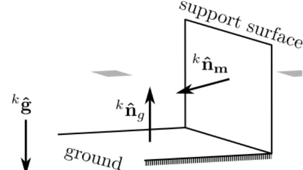
The depth sensor, however, has no direct way of measuring either the gravity nor the magnetic field of the environment. It is still possible to estimate these vectors in the local frame of this sensor if they are in some manner associated with the geometric features of the world. That can be accomplished by scanning a planar surface orthogo-nal to the gravity field (whose normal, kˆn
g, will be parallel tokˆg), and another planar
surface non parallel to the previous one, which we will refer to as the support surface. Both surfaces are illustrated by Figure 3.3.
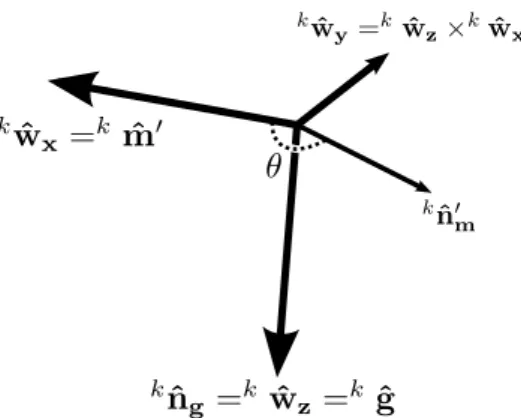
After orthogonalizing the normal of the support surface,knˆ
m, with respect tonˆg,
we obtain the vector knˆ′
m. As is illustrated by Figure 3.4, this vector can be thought
of as kwˆ
x after a rotation of a constant angle θ around the axis knˆg (which is the
18 Chapter 3. Methodology
Figure 3.4: World coordinate frame with respect to the depth sensor during the cal-ibration process. The axis kˆn
g is estimated from a planar surface orthogonal to the
gravity, and the axis knˆ′
m is obtained from orthogonalizing the normal of the support
surface with respect tokˆn
g.
kˆn′
m =Rθ,knˆ
g
kwˆ
x,
where the notation Rα,v specifies a rotation of an angle α about an arbitrary axis v.
Thus, the attitude of theworld with respect to the depth sensor can be expressed by
w
kK
−1
= [kmˆ′ kˆg
×kmˆ′ kˆg], kmˆ′ =R−1
θ,knˆ
g
knˆ′
m. (3.2)
Notice that it is still necessary to know the angle θ in order to calculate the rotationw
kK. In order to find this angle, we must consider the nature of the calibration
matrix k
mR = wkK
−1 w
mM. Since it represents a constant rigid transformation, we can
say thatk
mR=wkK
−1
t w
mMt, regardless of the time instant t. Therefore,θ can be found
as the solution to the non-linear system given by
w
kK
−1
ti
w
mMti =
w
kK
−1
tj
w
mMtj ∀ ti 6=tj. (3.3)
3.1. Extrinsic Calibration of the Sensors 19
θ= argmin
α
s X
ti
X
tj6=ti
kw
kKti(α) −1 w
mMti−
w
k Ktj(α) −1 w
mMtjk
2, (3.4)
whereKt(α)gives the attitude of the depth sensor with respect to the world at instant
t, assuming that the angle θ from Equation 3.2 is α.
After we have an estimate for θ by solving Equation 3.4 (which we computed by using the Nelder-Mead simplex, as it is a derivative-free method), it is possible to calculate the calibration matrix. Since we can compute an estimation of k
mRfrom each
measurement made by the depth sensor, we have to combine all these estimates into a single, reliable estimate of k
mR.
For each one of the captured attitudes, we have k
mR1 = wkK− 1 1
w mM1,
k
mR2 =
w
kK
−1 2
w
mM2, . . .,
k
mRtn =
w
kK
−1
tn
w
mMtn. The final rigid rotation between the sensors is
estimated as the average of all these rotations. Our approach to the rotation averaging problem consists of firstly converting all rotation matrices to quaternions. Due to the fact that two unit quaternions q and −q represent the same rotation, a naïve averaging by adding and normalizing quaternions would be subject to spurious results. Nevertheless, this can be avoided if the average is made between quaternions that have an angular distance shorter than or equal to 90◦, which is given by their dot product.
Finally, we perform a spherical linear interpolation (SLERP) [Shoemake, 1985] in an incremental fashion similar to the running average algorithm, which will produce the final averaged rotation, which we convert back to the matrix form (quat2dcm). This process is illustrated by Algorithm 1.
Algorithm 1 Rotation Averaging Require:
1: A set of quaternions q1,q2, . . . ,qn representing several noisy estimates of the rigid
rotation k
mRbetween the MARG and the depth sensor.
Ensure:
1: The average rotation matrix kmR. 1: qf ←q1
2: for i←2, n do
3: if qf ·qi <qf · −qi then
4: qi ← −qi
5: end if
6: qf ← slerp(qf,qi,
1
i)
7: end for
20 Chapter 3. Methodology Front-end Back-end Attitude Estimation Coarse Alignment Keypoints Detection Descriptor Extraction Keypoints Matching Photoconsistent Alignment Optimization Find loop correspondences Optimize graph Is Keyframe?
Yes Align to closest
keyframe Depth Sensor MARG Sensor Frame Pose Environment Map
Figure 3.5: A high-level overview of the proposed registration approach. The front-end is divided into three pairwise registration levels. Their alignment result is refined to a key frame level by a backend, which saves all locally consistent poses. These poses are later processed by a SLAM optimizer, which generate the globally consistent final map.
3.2
Point Cloud Registration
We propose a registration technique that consists of a coarse-to-fine alignment pipeline. This decision allows us to compute high quality transformation between adjacent point clouds with a small computational impact, since different pipeline stages can be par-allelized with a producer-consumer design. Also, the transformations found by coarser levels reduce the number of iterations required by finer levels to find their optimal solutions. The diagram on Figure 3.5 depicts a high level view of our approach.
The proposed algorithm starts by performing the keypoints detection and de-scriptor extraction for the first point cloud received. Then, for each new point cloud captured by the depth sensor, the whole pipeline is executed, whilst the alignment pro-cesses are performed between the latest two point clouds in a pairwise fashion. Each alignment level will be described in detail in the following subsections.
3.2.1
Front-end
3.2. Point Cloud Registration 21
point clouds. We use the orientation filter proposed by Madgwick et al. [2011] to fuse data coming from sensors in a MARG device. Their methodology uses the gyroscope, accelerometer and magnetometer to estimate the MARG attitude with respect to a fixed world frame specified by the gravity and earth’s magnetic field. We have chosen this approach due both to its stability and low computational requirements.
In an independent step, we find a set of SURF keypoints [Bay et al., 2008] from the most recent image. We have chosen the SURF detector based on the fact that it was capable of extracting several hundreds of good quality features from images of our experiment, even during the presence of some blurring due to camera motion. We also label these keypoints with BASE descriptors [Nascimento et al., 2012]. This descriptor is computed by using both intensity and geometry information, which makes them more robust to variations in lighting conditions and textureless scenes.
3.2.2
Keypoint Matching
In order to quickly match keypoints between a pair of frames, we developed a keypoint matching strategy that takes into account a prior knowledge of the displacement be-tween them. The rotation bebe-tween these frames can be approximated by a quaternion calculated with data from the MARG sensor, and the translation can be roughly es-timated by finding any pair of corresponding keypoints between the two frames being aligned.
Let k
mR be the extrinsic MARG/Depth sensor calibration matrix computed as
described in the previous section, and w
mMt be the MARG attitude at the t-th frame
as reported by the orientation filter. If the sensors were perfectly synchronized and the MARG sensor were not susceptible to noise and interference, the attitude of the t-th frame with respect to the (t−1)-th frame, kt−1
kt K, would be given by
kt−1
kt K= (
w mMt−1
k
mR
−1
)−1 w
mMt
k
mR
−1
.
In practice, this equation doesn’t yield an exact attitude due to problems such as noise from the MARG sensor, small extrinsic calibration errors and the lack of synchrony between MARG and RGB-D sensor. Furthermore, it only accounts for rotation, leaving the translation unknown. We tackle these issues by combining the estimated attitude with a maximum sensor motion speed assumption. Given a keypoint
22 Chapter 3. Methodology
a spherical shell defined by the parametric equation
(kt−1
kt K)
−1 kt−1k+ˆrvmaxdt,
where the parameterˆr is a unit vector, vmax is the maximum motion speed assumed,
and dt is the elapsed time separating the acquisition of those frames.
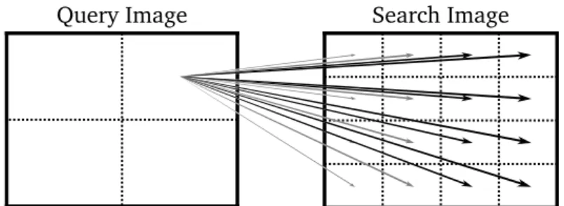
Considering the maximum speed assumption, our matching approach starts by selecting a subset of keypoints from the(t−1)-th frame in order to keep the compu-tational requirements low. This procedure, which we callsubsample on Algorithm 2, is done by selecting the N most prominent keypoints, where keypoints are compared according to their response to the SURF detector. Then, for each keypoint, we search for correspondences on the t-th image. To compute the set of matching candidates from the t-th frame, we perform a radius search for keypoints around a center given by(kt−1
kt K)
−1 kt−1k and radius length of vmaxdt. On Algorithm 2, the radius search
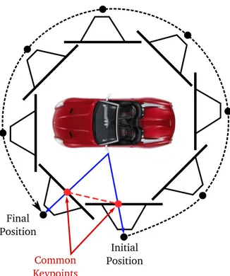
op-eration is presented asradiusSearch(kdTree, center, radius). Each candidate from the returned set has an associated vectort, which represents a possible translation between the two point clouds. These keypoints are referred to as support keypoints, and are connected by a red line in Figure 3.6.
We proceed by comparing all combinations between an arbitrary kt−1ki and its
corresponding results from the radial search. For each pairing, we have a different t
that, together with the attitude guess from the MARG sensor, provide an estimation of the pose of point cloudt with respect to point cloud t−1. Then, in order to refine this estimate, for all remaining keypoints kt−1k
l (with l 6= i), we perform a nearest
neighbor search in the t-th frame around the point given by (kt−1
kt K)
−1 kt−1k
l+t – we
have found that three neighbors is typically a good compromise between computational performance and alignment quality. The neighbor that best matches the current key-point is then defined as its pair. Once we have a correspondence for every keykey-point subsampled from the (t−1)-th frame, we calculate the Hamming distance between the binary descriptors of the matched keypoints. The distances are used to calculate a score of the current pairing configuration. We repeat this process from the beginning for all possiblekt−1k
i, and chose the set of pairing configurations with the smallest total
score, which is computed by the summation of all pair scores.
3.2. Point Cloud Registration 23
coarse alignment procedure.
Algorithm 2 Keypoint Matching Require:
1: Two sets of keypoints kt−1k={kt−1k1, . . . ,kt−1kn} and ktk={ktk1, . . . ,ktkm} from
the (t−1)-th and t-th frames, respectively, with their corresponding descriptors. 2: The attitude of the depth sensor at the instant i with respect to its orientation at
the moment t−1, kt−1
kt K.
Ensure:
1: The pose of the depth sensor at the instant t with respect to the instant t −1,
kt−1
kt P
2: The score of the best matching configuration.
1: kt−1˜k← subsample(kt−1k)
2: bestScore ← ∞
3: for all kt−1˜kl ∈kt−1˜kdo
4: kt˜k←radiusSearch(ktk,(kt−1
kt K)
−1 kt−1˜kl, vmax·dt)
5: for all kt˜k
l∈kt˜kdo
6: score ← hammingDistance(descriptor(kt−1˜k
l), descriptor(kt˜kl))
7: matches ← {(kt−1k˜l, kt˜kl)}
8: t←kt˜k
l−( kt−1
kt K)
−1 kt−1˜k
l
9: for all kt−1˜k
m ∈kt−1˜k|kt−1˜k
m 6=kt−1k˜
l do
10: c←(kt−1
kt K)
−1 kt−1˜k
m+t
11: neighbors ←KNNSearch(ktk, c,AMOUNT_NEIGHBORS)
12: kt˜k
m ← bestNeighbor(neighbors)
13: hamming← hammingDistance(descriptor(kt−1k˜
m),
descriptor(kt˜k
m))
14: if kc−kt˜k
mk ≤DISTANCE_THRESHOLD then
15: score ←score + hamming 16: matches← matches ∪ {(kt−1k˜
m,ktk˜m)}
17: end if
18: end for
19: score ←score/size(matches)2
20: if bestScore > scorethen 21: bestScore ← score
22: kt−1
kt P←poseFromPCA(matches)
23: end if 24: end for 25: end for 26: return (kt−1
24 Chapter 3. Methodology
Algorithm 2 has a time complexity of O(p(√q+M) logq+p2
(M√q)), where:
• p is the number of keypoints in kt−1k˜ (can be set to a maximum limit depending
on the subsampling strategy);
• q is the number of keypoints in ktk;
• √q+M is the time complexity of a radius search over a KD-Tree, where M is the expected number of returned nodes (this term is directly proportional to the translational uncertainty, given by vmax·dt);
• M√q is the time complexity of the KNN search on ktk.
In order to keep the computational cost of search operations low, we store the set of keypoints ktk in a KD-tree. The construction cost, O(qlogq), does not represent a
significant impact to the algorithm, since we typically deal with a number of keypoints
q <2000, when the SURF detector is employed.
Our keypoint subsampling approach takes into account two major factors. Firstly, we determine a maximum number of keypoints that the setkt−1k˜ might contain based
on their detection score. Secondly, we only sample keypoints whose distance to the camera is below a threshold. The reason for this second factor is the fact that farther points tend to be too noisy, which would cause a negative impact towards the pose estimation algorithm. Typically, this threshold is 3.5m for RGB-D sensors.
The main difference between the designed matcher and existing brute force tech-niques is that we apply a transformation to the keypoint around which a neighbor search will be performed. Therefore, after the transformation, the keypoint will lie closer to its correspondent. Also, the distance threshold used after the KNN search can be set to very tight values in order to preserve euclidean constraints, reducing the need for an explicit outlier removal. It is important to notice that the transformation that precedes the radius search doesn’t necessarily need to be a rotation. As we will discuss later on, this transformation will also contain a translation when the match-ing is made between frames with relatively large displacements (which happens every time on the back-end of our methodology, when it tries to align regular frames to key frames).
3.2.3
Photo Consistent Alignment
3.2. Point Cloud Registration 25
Figure 3.6: Keypoint correspondences found by our keypoint matching approach. The red line connects support keypoints, while the blue lines connects the remaining key-points. Although there were hundreds of matched keypoints on this pair, we selected a small set of pairs for the sake of clarity. The figures depict a region captured during our experiments.
quickly corrected by a geometry-based registration. However, such approaches have high computational requirements and may be compromised by the lack of geometric features from some environments. On the other hand, the acquired frames often con-tain a substantial amount of color information, which can be densely used to further improve the alignment, which will help to correct for small displacements on pair-wise registration.
For this alignment stage, we have employed the methodology published by Stein-bruecker et al. [2011]. Given two point cloudsCa, Cb for which each point contains its
color estimate, and an initial guess b
aP˜ for the pose of frame a with respect to frame
b, their algorithm searches for a pose b
aPthat leads to the smallest difference between
the image from Cb and the image obtained from applying the perspective projection
to the points b
aPCa. In other words, at each iteration, it compares the projections
from both point clouds as if they were obtained from the sensor at the same spot. If the transformation b
aP is close to the actual displacement between these clouds, the
intersecting pixels of the compared images will be more similar to each other, as it can be seen on Figure 3.7.
Other pairwise alignment methodologies, such as Henry et al. [2010], commonly use the ICP algorithm during their fine alignment stage. We have chosen the photo consistent approach due to its high computational performance, even though it uses all available points, and the fact that it uses intensity as an evaluation metric.
26 Chapter 3. Methodology
(a) Point cloudt (b) Point cloudt+ 1
(c) Point cloudt+ 1 after alignment (d) Aligned point cloudt+ 1superposed with point cloudt
Figure 3.7: Given a coarse estimate for the pose of frame a w.r.t frame b, kt−1
kt P
′, the
photo consistency step finds a kt−1
kt P that minimizes the difference between figs. (a)
and (c).
matrix,kt−1
kt P
′, which is combined into the global sensor posek1
ktPby the matrix product
k1
ktP=
k1
kt−1
Pkt−1
kt P
′.
This combined sensor pose is the input to the back-end, which will then refine it to a globally consistent pose.
3.2.4
Sampling Key frames and Graph Optimization
3.2. Point Cloud Registration 27
There are several entities that can lead to accumulated errors between frames, for instance:
• The sensor discretization of the world makes it impossible for any alignment to be perfect;
• Depth and image warping due to lens distortion, leading to curvy representations of planes;
• Blurring both on depth and color images introduces geometric distortions that do not correspond to the real environment.
Consequently, the back-end must be capable of detecting overlapping regions between key frames, especially if they have a large temporal displacement. Such in-tersections happen when the sensor returns to a previously mapped region, which may be very difficult to detect, since uncertainty due to accumulated error can make the search space too large when matching temporally farther key frames.
Another reason to use the proposed back end is to prevent normal frames (that is, point clouds that are not distinct enough to be considered key frames) from diverging indiscriminately. This is achieved by aligning them to the closest key frame available. As it will be discussed in more details later on, this realignment operation is typically very fast, since drifting between key frames typically occurs at small scales. Also, the detection of the closest key frame doesn’t require the world representation to be globally consistent, because our key frame detection policy ensures that a key frametis always a good candidate for matching subsequent point clouds that are not considered key frames.
3.2.4.1 Key frame Detection
The criteria for determining whether a point cloud can be considered a key frame or not is of crucial importance to the registration system, as it is related to the quality of the alignments as well as the overall algorithm run time. A large amount of key frames may induce higher run times by cluttering the graph to be optimized, as well as increase the accumulated error after mapping the whole environment. On the other hand, a small number of key frames implies in a smaller intersection region between them (assuming they all cover the same volume), which makes alignment a more difficult task, increasing the chances for registration divergence.
28 Chapter 3. Methodology
and all other key frames. This allows us to address the divergence issue, since a good registration depends on the size of the overlapping region, but also gives control over the amount of key frames detected, which can be reduced by decreasing the intersection threshold.
To determine whether or not a given point cloudCtis a key frame, let C˜k be the
set of all point clouds categorized as key frames. At the beginning of the alignment procedure, this set will be initialized with the first point cloud available – i.e. the first point cloud acquired by the depth sensor is automatically categorized as a key frame. If C˜k is not empty, we perform a comparison between Ct and each Cl ∈ Cˆk.
This is done by transforming all the points fromCt to the reference frame of Cl, and
projecting these points to the projection plane that contains all points from Cl (by
multiplying them by the projection matrix of the depth sensor, and normalizing their resulting homogeneous coordinates). Since the depth sensor might have moved after
Cl was captured, some of the points from Ct will be likely to be projected outside of
the projection plane of point cloud Cl. If the number of points that fall inside this
projection plane is below a threshold, we define Ct as a key frame. This procedure is
detailed in Algorithm 3.
3.2.4.2 Alignment to Closest Key Frame
During the registration process, it is desirable that regular point clouds be consistent with their closest key frames. This reduces the drift effect, restricting the error accu-mulation to the process of incorporating new key frames – an error that will be further reduced by graph optimization, should a loop be closed. Since our goal is to perform this alignment quickly as well as to obtain a high quality registration, we solve it with a specialized version of the feature matcher previously described.
The alignment error between a regular point cloud and the most recently detected key frame is typically small enough that their estimated poses can be used as an initial guess for the alignment between them. This alignment is computed by a slightly modified version of the keypoint matcher algorithm previously described. Also, since we expect to have small displacement errors, it is possible to prune the search space for feature correspondences, thus speeding up the feature matcher algorithm. Hence, given a pose estimate ki
ktP
′ of the t-th point cloud with respect to the key frame (which was
captured at instant i), the radius search of the keypoint matcher receives all support keypointskik˜
l transformed bykkit
˜
3.2. Point Cloud Registration 29
Algorithm 3 Key frame Detection Require:
1: A candidate point cloud Ct and its pose kk1tP.
2: A set of key frames C˜k, and their corresponding poses P˜k.
3: A camera projection matrix K. Ensure:
1: A boolean variable indicating ifCt is a key frame; in which case,C˜k is updated to
contain it as well.
1: isKeyFrame ←true 2: for all Cl ∈C˜k do
3: intersection ←∅ 4:
5: for all pl ∈Cl do
6: p′l ←Kk1
ktP −1 k
1
klP pl
7: p′′
l ← homogeneousNormalize(p′l)
8: if (0, 0)≤p′′l ≤(FRAME_WIDTH, FRAME_HEIGHT) then
9: intersection ← intersection ∪p′′l
10: end if 11: end for
12: if size(intersection) ≥ INTERSECTION_SIZE_THRESHOLD then 13: isKeyFrame← false
14: break for 15: end if
16: end for 17:
18: if isKeyFramethen 19: C˜k ←C˜k∪Ct
20: end if
21: return (isKeyFrame,C˜k)
ki
kt
˜ P′−1 =
ki
ktR
T −ki
ktR
T
t 01×3 1
!
,
where ki
ktRand tare, respectively, the rotation matrix and translation vector of
ˆ Pkt. The pose ki
kt
˜
P′ can be computed by using the global pose of point cloud t, k1
ktP
and the global pose of the key frame i, k1
30 Chapter 3. Methodology
transformations between all frames that preceded them:
k1
ktP=
t
Y
j=2
kj−1
kj P,
k1
kiP=
i
Y
j=2
kj−1
kj P.
In this sense, ki
ktP ′ =k1
kiP −1 k
1
ktP.
Given the transformationki
ktPresulting from the alignment between current point
cloud and the last detected key frame, the current stage outputsk1
kiP
ki
ktP, which stands
for the corrected, locally consistent, global pose of thet-th point cloud.
3.2.4.3 Optimizing Environment Graph and Closing Loops
In order to estimate a reliable representation of the environment, mapping trajectories that return to a previously visited region must be subject to loop closure techniques, which reduce significantly the accumulated error, an inevitable outcome of pairwise frame alignment.
This is done by associating a hypergraph to the key frame structure, in which each key frame is represented by a vertex, and each keypoint correspondence between them becomes an edge, as shown in Figure 3.8. Since our goal is to perform environ-ment mapping with 6 degrees of freedom in terms of sensor motion, this framework can be processed by the methodology proposed by Borrmann et al. [2008], which was an extension of a graph optimization framework for 2D scans with 3 degrees of freedom [Lu and Milios, 1997]. The latter takes as input a graph in which each vertex represents the sensor’s pose Xi =
x y θ (which may be estimated by pairwise registration of all previous point clouds), while edges between them contains the measured dis-placement between these poses Di,j =
∆x ∆y ∆θ (typically obtained from the alignment between those vertices). If all scans were perfectly matched and there were no cumulative error, there should be no difference betweenXi−Xj andDi,j for any two
connected nodes i and j. When accumulated errors are present, however, the graph optimizer must seek to minimize this difference. Therefore, its fitness function is given by the following Mahalanobis distance:
X
(Xi−Xj −Di,j)TCi,j−1(Xi−Xj −Di,j),