www.atmos-chem-phys.net/10/9761/2010/ doi:10.5194/acp-10-9761-2010
© Author(s) 2010. CC Attribution 3.0 License.
Chemistry
and Physics
Downscaling of METEOSAT SEVIRI 0.6 and 0.8 µm channel
radiances utilizing the high-resolution visible channel
H. M. Deneke1,2and R. A. Roebeling1
1Royal Netherlands Meteorological Institute, Postbus 201, 3730 AE De Bilt, The Netherlands 2Meteorological Institute, University of Bonn, Auf dem H¨ugel 20, 53121 Bonn, Germany
Received: 11 January 2010 – Published in Atmos. Chem. Phys. Discuss.: 23 April 2010 Revised: 15 September 2010 – Accepted: 1 October 2010 – Published: 18 October 2010
Abstract. An algorithm is introduced to downscale the 0.6
and 0.8 µm spectral channels of the METEOSTAT SEVIRI satellite imager from 3×3 km2(LRES) to 1×1 km2(HRES) resolution utilizing SEVIRI’s high-resolution visible channel (HRV). Intermediate steps include the coregistration of low-and high-resolution images, lowpass filtering of the HRV channel with the spatial response function of the narrow-band channels, and the estimation of a least-squares linear regression model for linking high-frequency variations in the HRV and narrowband images. The importance of account-ing for the sensor spatial response function for matchaccount-ing re-flectances at different spatial resolutions is demonstrated, and an estimate of the accuracy of the downscaled reflectances is provided. Based on a 1-year dataset of Meteosat SEVIRI images, it is estimated that on average, the reflectance of a HRES pixel differs from that of an enclosing LRES pixel by standard deviations of 0.049 and 0.052 in the 0.6 and 0.8 µm channels, respectively. By applying our downscal-ing algorithm, explained variance of 98.2 and 95.3 percent are achieved for estimating these deviations, corresponding to residual standard deviations of only 0.007 and 0.011 for the respective channels. For this dataset, a minor misregistra-tion of the HRV channel relative to the narrowband channels of 0.36±0.11 km in East and 0.06±0.10 km in South direc-tion is observed and corrected for, which should be negligible for most applications.
Correspondence to:H. M. Deneke ([email protected])
1 Introduction
Accurate information on cloud properties is a prerequisite for understanding the influence of clouds on the Earth radi-ation budget and the global hydrological cycle. Due to their dominant role as forcing of the surface energy budget, accu-rate information on surface radiative fluxes in cloudy condi-tions is of particular interest (Woods et al., 1984; Wielicki et al., 1995). Passive meteorological satellite imagers pro-vide important information for investigating cloud proper-ties (Stephens and Kummerow, 2007), and for quantifying their influence on solar (Deneke et al., 2005) and thermal (Schmetz et al., 1990) radiation. Several projects generate data records of cloud properties, including the International Satellite Cloud Climatology Project (ISCCP, Rossow and Schiffer, 1991), the Pathfinder Atmospheres project (PAT-MOS, Jacobowitz et al., 2003), the MODIS project (Platnick et al., 2003), and the Satellite Application Facility on Climate Monitoring (CM-SAF, Schulz et al., 2009).
cause large random and systematic differences in cloud prop-erties such as optical thickness and liquid water path (Ore-opoulos and Davies, 1998; Deneke et al., 2009b), and cause uncertainties for the classification of cloud thermodynamic phase (Wolters et al., 2010). In particular, the spatial resolu-tion of SEVIRI’s narrowband channels is insufficient to re-solve small cloud structures. As demonstrated by Heidinger and Stephens (2001), unresolved spatial heterogeneity can cause errors in retrieved cloud properties large enough to ren-der them useless. To partly overcome this problem, Kl¨user et al. (2008) utilized the high-resolution broadband visible channel (HRV) with a sampling resolution of 1×1 km2 at nadir to study the lifecycle of shallow convective clouds.
In addition, the considered spatial (Greuell and Roebel-ing, 2009; Schutgens and RoebelRoebel-ing, 2009) and temporal (Deneke et al., 2009a) scales of variability have a strong im-pact on the correspondence of satellite and ground observa-tions, and thus the task of satellite product validation. D¨urr et al. (2010) conclude that the higher spatial resolution of-fered by the HRV channel has a beneficial effect on the qual-ity on retrievals of solar surface irradiance over the Alps due to their complex terrain.
In this paper, we want to demonstrate that the HRV chan-nel contains important additional information on small scale variability which can be utilized together with SEVIRI’s 0.6 and 0.8 µm channels for quantitative analysis. Cros et al. (2006) have demonstrated that the relationship between re-flectances from these two channels and the MVIRI (Meteosat Visible and InfraRed Imager) broadband visible channel on-board Meteosat-7 (Meteosat First Generation) is highly lin-ear and stable in time, due to the spectral overlap of these channels. Since the MVIRI channel of Meteosat First Gener-ation and the HRV channel of Meteosat Second GenerGener-ation have very similar spectral responses (Schmetz et al., 2002), their finding should also hold for the HRV channel, and in-dicates that the variations observed in the HRV reflectances will be strongly correlated to those observed in the 0.6 and 0.8 µm channel.
The goal of Cros et al. (2006) was to predict the broad-band channel reflectance from the narrowbroad-band channels so as to generate input for legacy applications based on MVIRI. In contrast, the purpose of this paper is to introduce a novel algorithm to estimate the reflectances of the 0.6 and 0.8 µm channels at the threefold higher spatial resolution of the HRV channel, by utilizing the HRV reflectances as predictor. As constraint, the statistical properties of the narrowband re-flectances should be preserved at their native channel reso-lution. Such methods are referred to as downscaling (Liu and Pu, 2008) in climate research or disaggregation (Walker and Mallawaarachchi, 1998) in geostatistics. Following Cros et al. (2006), we have decided to use image-wide linear models for simplicity, and neglect any scene-type dependen-cies. Other SEVIRI narrowband channels apart from 0.6 and 0.8 µm are ignored at the moment. This work nevertheless constitutes a first step towards producing higher spatial
reso-lution products from SEVIRI such as cloud water path (e.g., Roebeling et al., 2008) and solar surface irradiance (e.g., Deneke et al., 2008; M¨uller et al., 2009) over Europe.
In this paper, special attention is paid to some technical details which might affect the quality of our proposed algo-rithm. First, the spatial response of the SEVIRI channels does not correspond to the idealized form of a rectangular function, and the radiance field is significantly oversampled, as has been pointed out by Schmetz et al. (2002). This causes radiance contributions from a region significantly larger than the 3×3 km2sampling resolution (referred to as LRES in the following) of the narrowband channels, and the 1×1 km2 res-olution of the HRV channel (referred to as HRES). Thus, it is insufficient to use simple arithmetic averages of 3×3 km2 pixels to reduce the resolution of the HRV images to that of the narrowband channels, and the true sensor spatial response should be used instead. In addition, an accurate coregistra-tion of the LRES channels with the HRV channel is cru-cial for the quality of our downscaling scheme. Our algo-rithm uses frequency-domain methods based on the discrete Fourier transform for modeling the spatial response function of SEVIRI’s detectors (Markham, 1985) and to determine the image coregistration (Anuta, 1970). These methods have the advantage of being both mathematically elegant and compu-tationally efficient.
This paper is structured as follows. In Sect. 2, the in-strumental dataset is described. An outline of the proposed downscaling algorithm is given in Sect. 3, with some general background provided as Appendices. In Sect. 4, examples of results obtained with these methods are reported, and the ac-curacy of our method is demonstrated and discussed. Finally, conclusions and an outlook are given in Sect. 5.
2 Instrumental data
Meteosat Second Generation is the current series of Euro-pean geostationary satellites, which began operational data acquisition in January 2004 and is described in detail by Schmetz et al. (2002). Its Meteosat-8 and 9 satellites carry the SEVIRI imager as primary instrument, and are positioned above the equator at longitudes of 9.6◦E and 0.0◦W, respec-tively, at the time of writing. In operational service, the SEVIRI imager scans the complete disk of the earth with a 15 min repeat cycle. Meteosat-9 is currently the opera-tional satellite, while Meteosat-8 is used as hot stand-by, and scans a subregion with a 5 min repeat cycle in Rapid Scan Mode. SEVIRI has 3 narrowband solar channels (0.6, 0.8 and 1.6 µm), the broadband HRV channel (0.4–1.1 µm), and 8 thermal infrared channels (3.9, 6.2, 7.3, 8.7, 9.7, 10.8, 12.0 and 13.4 µm).
Table 1.Central wavelengthλ0, channel widthδλ(both in nm), and band-averaged extraterrestrial solar spectral irradianceφC(W/m2/µm)
at a sun-earth distance of 1 astronomical units for the SEVIRI radiometers onboard the Meteosat-8 to 10 satellites and for the 0.6 µm (VIS006), 0.8µm(VIS008) and HRV channels, calculated from the spectral response functions provided by EUMETSAT (2006b) and the solar spectrum of Gueymard (2004). The central wavelengthλ∗0and channel width δλ∗ for the spectral response weighted by the solar spectrum are also listed.
Meteosat VIS006 VIS008 HRV
λ0 δλ φC λ0 δλ φC λ0 δλ φC
8 640.2 74.5 1594.8 809.3 57.3 1106.8 708.2 421.3 1395.6 9 640.3 73.4 1594.4 808.2 57.3 1109.6 706.4 422.2 1400.1 10 638.2 70.9 1601.3 808.2 57.0 1109.5 707.0 428.7 1398.9
λ∗0 δλ∗ - λ∗0 δλ∗ - λ∗0 δλ∗
-8 639.0 73.7 – 808.6 54.6 – 669.7 388.6 – 9 639.1 72.5 – 807.4 55.1 – 668.0 387.5 – 10 637.0 70.3 – 807.5 54.4 – 668.2 385.0 –
0.4 0.6 0.8 1.0 1.2
0.0
0.2
0.4
0.6
0.8
1.0
(a)
Wavelength [ µµm ]
Spectral response
HRVIS VIS006 VIS008 MS7_VIS
0.4 0.6 0.8 1.0 1.2
0.0
0.2
0.4
0.6
0.8
1.0
(b)
Wavelength [ µµm ]
Weighted spectral response
HRVIS VIS006 VIS008 MS7_VIS
Fig. 1. Spectral response functions of the Meteosat-9 SEVIRI ra-diometer for the 0.6 µm (red), 0.8 µm (green) and HRV channel (black) (EUMETSAT, 2006b). The central wavelength of each channel is marked by a thick colored line, and the spectral region covered by the channel width has been shaded. The response of the Meteosat-7 MVIRI solar channel is also included for compari-son (blue). The normalized spectral response functions are plotted in(a), while the spectral response functions weighted by the solar spectrum of Gueymard (2004) are displayed in(b). The solar spec-trum is added as dotted line to both plots.
are listed in Table 1 for Meteosat-8 to 10. The SEVIRI imager acquires pixels at sampling resolutions of 1×1 km2 and 3×3 km2for the high-resolution visible channel (HRV) and the narrowband channels, respectively. It has to be re-alized, however, that SEVIRI has a lower optical resolution and oversamples the reflectance field by a factor of about 1.6 at both LRES and HRES resolution (Schmetz et al., 2002). Thus, the effective area contributing to an individual pixel radiance is significantly larger than the sampling resolution. This is illustrated in Fig. 2b, which displays the response of the SEVIRI detectors to a unit pulse of radiance as function of distance from the pixel center, and shows significant con-tributions from regions outside the nominal sampling resolu-tion. Its calculation is explained in Sect. 3.3
3 Methodology
This section presents our proposed downscaling algorithm. In overview, it consists of the following sequence of steps:
1. coregistration of the HRV and the narrowband images to ensure an optimal alignment of the satellite images; 2. Filtering of the HRV image with the spatial response
function of the LRES detectors, to separate the image into low-frequency variability resolved at LRES scale, and unresolved high-frequency variability;
3. Determination of a least-squares linear model based on LRES reflectances to link the HRV, 0.6 and 0.8 µm channels as proposed by Cros et al. (2006);
variability from step 2 as predictor; least-squares esti-mators are used to overcome the underconstrained na-ture of this inversion;
5. trigonometric interpolation of the 0.6 and 0.8 µm chan-nels to obtain images at HRES resolution, but lacking high-frequency variability;
6. addition of high-frequency variability found in step 4 to the 0.6 and 0.8 µm HRES images as estimate of the true HRES image;
More details about these steps are described in the follow-ing. A brief summary of the Fourier Transform is given first. Then, its application to the tasks of image coregistration, and to the separation of low- and high-frequency spatial varia-tions is described. Next, the determination of a linear model for linking the 0.6 and 0.8 µm with the HRV radiances, and for inverting this model is outlined, in order to estimate the unresolved variability in the narrowband channels. Finally, some implementation details are noted.
3.1 The Fourier transform
A 2-D imagefx,yconsisting ofNx×Nydiscrete digital
sam-ples is considered here. The sampling frequency limits the maximum frequency which can be captured by the image. This limit is equal to half the sampling frequency, and is called the Nyquist frequency.
The discrete Fourier transformfbk,l of the 2D image
con-sists of Nx×Ny samples, and projects the image onto an
orthonormal basis set of sinusoidal waves with circular fre-quencies of ωk= 2Nπ k
x , k∈0...(Nx−1) and ωl=
2π l
Ny, l∈
0...(Ny−1). Vectorsωandxcan be used to compactly rep-resent the 2-dimensional case of the Fourier transform.
Fourier analysis implicitly treats signals as periodic. To avoid the influence of resulting discontinuities at the edges, it is common practice to subtract the mean and to use a win-dow function to reduce the deviations from zero at the edges of the image prior to the Fourier transform. Here, the Tukey window with a transition width of 25 percent along both di-mension is used. A detailed discussion of window functions and their relevance for Fourier analysis can be found in Har-ris (1978).
3.2 Image coregistration
Our approach for image coregistration relies on the so-called Fourier shift theorem: the Fourier transform of a function
f′(x)≡f (x−x0)shifted by an offsetx0versus the original functionf is given by
b
f′(ω)=f (bω)exp[iωx0]. (1)
Thus, the translation of a function changes only the complex phase of its Fourier transform, while leaving its amplitude
invariant. To align a satellite imagegrelative to an imagef, a functionhis defined as follows:
h≡bgfb∗=kbgkkfbkexpi(arg(bg)−arg(f ))b . (2) Here, the arg operator determines the phase of a complex number. Ifg(x)=f (x−x0), arg(h)will only depend on the shiftx0=
x0
y0
according to:
arg(h)=arg(f )b+ωx0−arg(f )b=2π
k Nx
x0+
l
Ny
y0
. (3)
In our case, the complex phase ofh is calculated from the Fourier transforms of the HRV and the narrowband images for individual SEVIRI scenes. A linear combination of the 0.6 and 0.8 image is used for this purpose, as is explained in Sect. 3.4. Fourier coefficients of the HRV image beyond the Nyquist frequency of the LRES images are ignored. Theoret-ically, Eq. (3) suggests a perfect linear relation. In practice, deviations from this equation are expected due to image dif-ferences and the discrete sampling. A 2-dimensional linear least-square regression of Eq. (3) nevertheless provides a re-liable and accurate estimate of the image shiftsx0 andy0.
As noise introduces larger phase errors for complex numbers with small modulus, a weighted linear regression is used here with the modulus used as weight. Once the shift has been found, the HRV image is aligned to the narrowband images by multiplying its Fourier transform with the complex factor exp[−iωx0]. It should be noted that this method is thus able to correct even for a fractional shift of the pixel resolution.
3.3 Spatial response of a detector
To separate high-frequency variability not resolved at LRES scale from low-frequency variability in the HRV channel, the effects of the spatial response function of the LRES detectors need to be considered.
We assume that the signalSof an individual SEVIRI pixel can be determined by spatial integration of the radianceL(x) reflected from the earth surface at locationx, weighted by a functionw(x−x0)which characterizes the spatial response of the detector:
S(x0)= Z
A
w(x−x0)L(x)dx
=(w∗L)(x0). (4)
signal processing. In principle, it is possible to determinew
by moving a point source of unit radiance across the detec-tor field of view. In the second line of Eq. (4), the symbol ∗denotes the convolution of two functions. To evaluate this convolution efficiently, the Fourier convolution theorem can be used, which states that the convolution in spatial domain is equivalent to a multiplication in frequency domain. Hence, the impact of a detector’s spatial response on scene sampling can be accounted for by a simple multiplication of the Fourier transforms ofLandw.
The modulus of the Fourier transform ofw is called the modulation transfer function (MTF), and describes the ratio of the amplitudes of a sinusoidal wave before and after pass-ing through an optical system. The MTF is thus a commonly used quantity to characterize the spatial resolution of optical systems. Figure 2a displays the average MTFs of Meteosat-9 SEVIRI’s 0.6, 0.8 µm and HRV channels as reported by EU-METSAT (2006a). As the MTF of the narrowband channels differ only slightly, they have been averaged, and any devia-tions between the two channels and individual detectors are neglected. The figure also illustrates the difference in spatial response in North-South and East-West direction. In Fig. 2b, the point spread functionwis shown, which has been calcu-lated from the MTF by the inverse Fourier transform. Even symmetry about the origin has been assumed forwto ensure that bothwitself and its Fourier transform are real functions. This makeswa zero-phase FIR filter, a property which im-plies that the original and the filtered image remain unshifted relative to each other.
It has to be realized that the MTFs and point spread func-tions shown in Fig. 2 are in fact determined by the angu-lar resolution of the individual SEVIRI detectors. The spa-tial scales and frequencies specified in this paper refer to the spatial resolution at nadir, and a reduction in resolution for off-nadir viewing geometries needs to be accounted for sepa-rately. As the angular resolution of the HRV and narrowband channels remains constant over the entire SEVIRI disk, the change in viewing geometry does not affect our downscaling algorithm.
In our downscaling algorithm, the HRV image is filtered with a low-pass filter to simulate an LRES image. This filter-ing operation is carried out in the frequency domain by mul-tiplication of the Fourier transform with an effective MTF. This is obtained from the average MTF of the 0.6 and 0.8 µm detectors, divided by the HRV MTF. The division is done to account for the fact that the HRV image is already smoothed due to its imperfect spatial response, and avoids a separate de-convolution step.
3.4 Linear relation of channel radiances
Our paper builds upon the study of Cros et al. (2006). Based on collocated satellite images from Meteosat-7 and Meteosat-8, they have demonstrated that SEVIRI’s 0.6 and 0.8 µm channel radiances can be used in a linear model to
0.01 0.02 0.05 0.10 0.20 0.50 1.00
0.0
0.2
0.4
0.6
0.8
1.0
(a)
Spatial Frequency [km−−1 ]
Modulation Transfer Function
HRES NS HRES EW LRES NS LRES EW
−4 −2 0 2 4
0.0
0.4
0.8
(b)
Distance [km]
Normalized Spatial Response
Fig. 2. (a)Modulation transfer function (MTF) of the 3×3 km2 low-resolution(LRES) 0.6 and 0.8 µm channels and the 1×1 km2 high-resolution visible channel (HRES) for Meteosat-9 in North-South (NS) and East-West (EW) directions (EUMETSAT, 2006a). The Nyquist frequencies corresponding to the sampling resolution are shown in grey, with values of 16km−1 (LRES) and 12km−1 (HRES).(b)Point spread function of the SEVIRI detectors recon-structed from the MTFs (see text for details), as a function of dis-tance from the pixel center. In grey, a perfect step response at LRES and HRES sampling resolution is also shown.
predict the broadband solar channel of the MVIRI instru-ment onboard Meteosat-7 with high accuracy. They motivate this assumption with the overlap of the narrowband channels and the MVIRI broadband channel. As the spectral response of SEVIRI’s HRV channel is similar to the MVIRI broad-band solar channel (Schmetz et al., 2002), we also adopt this assumption. Instead of radiances, however, the LRES reflectances of the 0.6 µm (r06), 0.8 µm (r08), and the HRV
(rH) channels are used here in the linear model:
rH=a r06+br08. (5)
In this equation,a andb are fit coefficients determined by least -squares linear regression. Choosing reflectances in-stead of radiances only alters the fit coefficients as reflectance and radiance co-vary linearly for a given solar zenith angle. No offset is incorporated into the linear model, as it has been found to cause only a negligible improvement in model qual-ity.
Fig. 3. Region of the SEVIRI field of view used for this paper, consisting of 1024×512 pixels. Also shown are contours of latitude and longitude in blue, and of the amplitude of the window function used for Fourier analysis in red. The subregion shown in Fig. 4 is marked by a black shaded rectangle.
ηof a satellite detector. Figure 1 graphically displays these quantities for the SEVIRI instrument on Meteosat-9, while numerical values as reported by (EUMETSAT, 2006b) are listed in Table 1 for Meteosat-8, 9 and 10. Both narrow-band channels lie completely within the range of the HRV channel. Weighting by the solar spectrum reduces the width of all channels, and shifts the channel centers towards the maximum of the solar spectrum. Both effects are most pro-nounced for the HRV channel due to its large width.
These numbers also reveal that both narrowband channels cover less than a third of the solar energy contained in the spectral range of the HRV channel. Hence, channel overlap is only a partial explanation of the high accuracy of the lin-ear model reported by Cros et al. (2006). A high degree of autocorrelation of the reflectances across the spectral region of the HRV channel is thus also required. This spectral au-tocorrelation also ensures that the results presented here are relatively insensitive to the width of the narrowband chan-nels of the SEVIRI instrument, and motivates our choice of reflectance instead of radiance as variables in Eq. (5).
3.5 Estimation of unresolved variability
In contrast to Cros et al. (2006), our aim is to estimate high-frequency variations in both narrowband channels from cor-responding HRV variations, by inversion of Eq. (5). Mathe-matically, it is impossible to determine two unknowns from one linear equation, as this is an underconstrained problem. Due to a strong correlation of the 0.6 and the 0.8 µm channel,
accurate estimates can nevertheless be obtained using stan-dard least-squares estimators. The goal is to find the optimal slopes S(r06) andS(r08)for linking high frequency
varia-tions1rin the HRV and the narrowband channels in a linear model:
1r06/08=S(r06/08)×1rH. (6)
In Appendix B, general expressions for calculating the slopes
S(r06/07)which minimize the least-squares deviations are
de-rived, based on bivariate statistics. Also, the expected frac-tion of explained variance for this linear model is given in Eq. (B8). Both formulae depend only on the coefficients
a andb from Eq. (5), the correlation between the 0.6 and 0.8 µm reflectance, and the ratio of the variances of both channels. It has to be recognized, however, that these pa-rameters might vary with the spatial scale of variability, and that we require their values at HRES scale here, which is not available from SEVIRI. To still obtain an estimate of their value, and to minimize errors caused by scale mismatch, both parameters are calculated considering the smallest re-solved scale of variability present in the LRES images. For the purpose of parameter estimation, we thus use difference images obtained by subtracting a shifted from an unshifted image, with shifts of 1 pixel applied in both the North-South and East-West direction. This procedure corresponds to a highpass filter, with maximum filter response at the Nyquist frequency of the LRES images, which is half the sampling frequency, and thus the maximum frequency captured in the LRES images.
3.6 Implementation details
At the beginning of this section, the sequence of steps com-prising the downscaling algorithm has been listed. In prac-tise, the individual steps of our implementation are not inde-pendent as suggested by that list. As first step, the HRV im-age is shifted relative to the narrowband channels to account for misregistration. As reference, the linear combination of the 0.6 and 0.8 µm channel given by Eq. (5) is used. The re-quired coefficients are only found in step 3, however. In ad-dition, if the HRV pixel shift exceeds half a pixel, the subre-gion of the HRV is changed to minimize the phase shift used for the Fourier-based image alignment. Therefore, mean val-ues of the linear weights and pixel shifts are used initially, and steps 1 to 3 are carried out iteratively until the remaining image misregistration is smaller than half a HRV pixel size. Most of the time, this condition is met already by the first iteration.
4 Results and discussion
Table 2.Annually averaged parameters (Mean) and their standard deviation (SDev) obtained by the downscaling algorithm. This includes: the slopesaandbof Eq. (5), and the explained variance EV (Eq. 5) of the underlying linear equation; the slopesS(r06)andS(r08)used to
scale high-frequency variations in the HRV channel to estimate unresolved variability in the 0.6 and 0.8 µm reflectance (based on Eq. B6); the explained variance EV(r06), EV(r08) of these estimates; and the correlation coefficient between variations in the 0.6 and 0.8µmreflectance.
Explained variances (EV) are listed in units of percent.
a b EV, Eq. (5) S(r06) S(r08) EV(r06) EV(r08) Cor(r06,r08)
Mean 0.667 0.368 99.7 0.949 1.000 98.5 95.6 0.945
SDev 0.025 0.020 0.1 0.036 0.041 0.5 1.6 0.020
A sub-region containing 1024×512 LRES pixels from SEVIRI’s field of view has been selected for our study, which is shown in Fig. 3. It covers Northern Africa, the Mediter-ranean Sea, and a large part of Europe. A smaller number of pixels in North-South than in East-West direction is used to limit the change in pixel resolution caused by the increase of satellite viewing angle away from the equator. The Tukey window function applied to the data prior to the Fourier transform is also shown by red contours, which corresponds to a cosine-shaped transition from 0 to 1 over 64 LRES els at the Northern and Southern edges, and 128 LRES pix-els at the Eastern and Western edge, respectively. One year’s worth of satellite scenes acquired at 12:00 UTC during 2008 has been analyzed. Due to Meteosat-9’s sub-satellite point at 0.0deg W, the time slot corresponds to the maximum so-lar top-of-atmosphere irradiance for the entire SEVIRI field of view. This yields a total number of 345 scenes from Meteosat-9, and 10 scenes acquired by Meteosat-8 operat-ing as backup duroperat-ing satellite anomalies of Meteosat-9. The remaining 10 scenes are missing or corrupted in KNMI’s archive.
Figure 4 shows the English channel and the Benelux states as example output in a SEVIRI scene acquired at 12:00 UTC on 26 June 2008. This subregion is marked in Fig. 3 by a black shaded rectangle. Panel (a) displays this scene in grey scales as observed by the HRV channel. Panel (b) shows the same scene using theday natural colorfalse-color composite described in detail by Lensky and Rosenfeld (2008) at LRES resolution. This scheme uses the 1.6, 0.8 and 0.6 µm spectral channels as red, green, and blue signals, respectively, and fa-cilitates the physical interpretation of the image, as it allows to easily distinguish different surface types, as well as ice and water clouds. Panel (c) shows this scene once more using the color scheme of (b), but based on the downscaled 0.6 and 0.8
µmspectral channels (the resolution of the 1.6 µm channel has been increased to HRES by sinc interpolation).
During that day, a high pressure ridge extended from the Azores over France and Germany with moderate summer temperatures and relatively dry air, and temporarily replaced hot and humid air masses. A low pressure system was lo-cated to the North of the British Isles. The satellite scene shows scattered fair-weather cumuli over South-Eastern
Eng-Fig. 4. Example output of the downscaling algorithm in compar-ison to standard SEVIRI images, based on a scene from 36 June 2008 of England, the British channel, north-eastern France, Bel-gium and the Netherlands. Panel(a)shows the HRV reflectance in grey levels, while(b)shows theday natural colorsRGB compos-ite of Lensky and Rosenfeld (2008) at standard SEVIRI resolution. Panel(c)is based on the downscaled 0.6 and 0.8 µm reflectances at HRV channel resolution, combined with an 1.6 µm image obtained by trigonometric interpolation.
Table 3.Effect of image coregistration and spatial averaging meth-ods on the explained variance (EV) and its standard deviation (SDev) for the linear model of HRV, 0.6 and 0.8 µm reflectance ex-pressed by Eq. (5) and given in percent. For a description of the different methods, see the text.
Ref LP48 3×3 1×1 5×5 NoCoReg
EV 99.68 99.08 99.04 96.83 94.60 99.61 SDev 0.11 0.28 0.27 0.94 2.32 0.14
interpretation of the image due to its use of multi-spectral information. Visually, panel (c) clearly demonstrates that our downscaling scheme is able to combine the advantage offered by the day natural color composite with the higher spatial resolution of the HRV channel. It could therefore be-come a valuable tool for assessing the synoptic situation in operational weather forecasting environments.
While these qualitative results are encouraging, a proper uncertainty analysis is required to judge the suitability of the downscaled reflectances as input for quantitative satellite re-trievals. For this purpose, two separate sources of uncertainty are considered, which are assumed to be statistically inde-pendent. The first source results from deviations from the linear model between the 0.6, 0.8 µm and HRV reflectance given by Eq. (5). The second source of uncertainty lies in the underconstrained nature of the downscaling problem, which has been discussed in Sect. 3.5 and is quantified by Eq. (B8). Average values of the required parameters have been calcu-lated for the entire dataset and are listed in Table 3.5.
As measure of uncertainty, the fraction of unexplained varianceU V is considered, which is related to the explained varianceEV byU V =1−EV. Assuming independent error propagation, the combined fraction of unexplained variance is given as the sum of the two individual fractions of unex-plained variance. Calculating the total unresolved variability based on the values given in Table 3.5, values of 1.8% and 4.7% are found, with corresponding values of total explained variance of 98.2% and 95.3% for the 0.6 and 0.8 µm chan-nels, respectively. Looking at the relative contributions to the uncertainty, fractions of 80.6% and 91.6% are attributable to the inversion carried out by Eq. (B6), and identifies it as the dominating source of uncertainty. The uncertainty is larger for the 0.8 µm than for the 0.6 µm channel, as its influence on the HRV channel is smaller, as is indicated by the value ofb
being smaller thanain Eq. (5).
Figure 5a displays the annual time series of the slopes
S(r06)andS(r08)calculated for individual satellite scenes.
To relate the fraction of unexplained variance to an estimate of the absolute accuracy of the downscaling algorithm, the increase in variance going from LRES to HRES resolution is needed. It is expressed as standard deviation by use of the square root of the variance here. Figure 5b shows annual
++++++++++++++++ ++++++ +++++++++++++++++++++++++ ++++++++++++++++++++++++++++++++++++++++++++++++++++++++++++++++++++++++++++++++++++++++++++++++++++ +++++++++++++++++++ ++++++++++++++++++++++++++++++++++++++++++++++++++++++++++++++++++++++++++++++++++++++++++++++++++++++++++++++++++++++++++++++++++++++++++++++++++ +++++++++++++++++++++++++++++++++++++++++++
0 50 100 150 200 250 300 350
0.8 0.9 1.0 1.1 1.2 (a)
Regression Slope [−]
xxxx x xxxxxxxx x xx xxxxxxxxx x x xxxxxxxxxxxxxxxxxxxx
xxxxx x xxxxxxx
x xxxxxxxxxxxxxxxxxxxxxxx
xxxxxxxxxxx x xxxxxx
xxxxxxxxxxxxxxxxx xxxxxxxxxxxxxxxxxxxxx
xxxxxxx xxxxxxxxxxxxxxxxxxxxxxxxxxxx
x x xxxxxxxxxxxxxxxxxxx
xx x xxxxxxxxxxx
xx x
xxxxxxxxxxxxx xxxxxxxxxx
xxxxxxxxx x xx xxxxx
xxxxxxxxxxxxxxxx x xxxxxxxxxxxxxxx
xx xxxxxxxx
x xxxxxxxxxxxxxxxxxxx
xxxxx xxxxxxxx
xxx xx xx x x xxxxxxxxxx
xxxxxxxx
VIS006: mean=0.95 sdev=0.04
VIS008: mean=1.00 sdev=0.04
+ ++ +++ + ++ + + ++++ ++ +++ ++ ++ + +++ ++ ++ + + + ++ +++ + +++ + + + + + + +++++ +++ ++ + ++ ++ + + +++ + + +++ + + + + + + + +++ + +++ ++ + ++ + + ++ ++ ++ + + +++++ + +++ +++ + + ++ +++++++ ++++++ + ++++ + +++++++++++ + ++++++++ + ++ + + ++++ +++ ++ + + + +++++ ++ ++ ++++ ++++ ++ + ++ ++++++ + +++ + + + + + ++ +++ ++++++++ + +++++ + +++++++++++ + ++ +++ +++++ ++ ++++ ++++ + + + + ++ +++ + ++ ++ + + + + ++ + + ++ ++ + + + + ++ +++ + + ++ + ++++ ++ + + + ++ ++ + + + ++++ + +++++ +++++ ++ +++++ + +++++++++++
0 50 100 150 200 250 300 350
0.02 0.04 0.06 0.08 0.10 (b) SDev(LRES−HRES) x xx
xxx x xx x x xxxx xx xxx xx xx x xxx x xxx x xx xx xxx xx xx x x x x x x xxxxx x x x xx xxx xx x x xxx x x xxx x x x x x x xxxx x xxxxxxxx
xx xx xx xx xx x xxxx x xxx xxx x x x x xxxxxxx
xxxxxx x xxxxx
xxxxxxxxxxx x xxxxxxxx
x xx x xxxxx xxxxx x x x xxxxx
xx
xx xxxx
xxxx xx xxxxxxxxxx
xxxxx x x x xx xxx xxxxxxxx x x xxxxxxxxxxxx
xx xx x xx xxx xxxx x xxx xx x xxxx
x x x x xx x x x x xx xx x x x x xx x x xx xx x x x x xx xxx x x xx x xx xx xx x x x xx xx x x x x xxx x
xxxxx xxxxx xx xxxxx x xxxxx xx xx xx * ** *** * ** * * **** ** *** ** ** * *** * **** * * ** ** * ** ** * * * * * * ***** ** * ** *** ** * * *** * * *** * * * * * **** * * ******** ** ** ** ** * * ***** * *** * *** * ** ******* ****** * ***** ********** ******* * ***** * * **** **** * * * ***** *** ** * * ** **** ** * ** * * ********** * * * ** *** ******** * ***** * ******* * *** * ** *** ***** ** **** **** * * * * ** * ** * ** ** * * * * ** * * ** ** * * * * ** *** * * ** * **** ** * * * ** ** * * * * *** * ***** ***** ** ***** * **** * ** ** **
VIS006: mean=0.049 sdev=0.009
VIS008: mean=0.052 sdev=0.012
HRVIS: mean=0.052 sdev=0.011
+ ++ ++++++++++++ ++++++++++++++ +++++++++++ + ++++++++ +++++++++++ + ++ +++ + +++ +++++ ++ +++++++++++++ + + ++++++++ +++ +++++++++ + ++++++++++++++++++++++++++++++++++++++++++ +++++++++ +++++++++++++++++++++++++++ ++ ++ ++++++ + ++++++++++++++++++++++++++++++++++++++++++++++++++++++++ ++++++ + +++++++++++ +++ ++ ++ + ++ +++++++++++++++++ + +++++++ + ++ ++ +++++++ ++++++++++++++ + +++++ +++ + ++++++++
0 50 100 150 200 250 300 350
0.000 0.005 0.010 0.015 0.020 (c)
Julian Day 2008
SDev(DSCAL−HRES) xxx xx x x xxx xxx x x xxxxxxxxxxxxxxxxx
x x x x xxxx x xx x x xxx x xxxxxx xx xxx xxx xxx x xx x xxxxx xx xx xx x x xxxxxxx x x xx x x xxxx xxxx x xxxx
xxxxxxxxxxxxxxxxxxxx xxx
x xxxxxxx xxxxxxx
x xxxxxxxxxxx
xxxxxxxxx xxxxx
xx xxxxxxxx
xxxxx x xx xx xx xxxx
xxxxx xxxxxxxx
x xxx
xx xxxxxxxxxxxxxx
x xxxxxx
xxx x xxxxxxxxxxx
xxxxxx x xxx x xxx xxxx xx x xxxx x x x x xxxxxxxxxxxx
xxxx x x x xx x xx xxxxx x x xx xx xx x x xxx x xx x x xx xxxxxx
xxxx x xxxxxxxxx
xx x
VIS006: mean=0.0065 sdev=0.0009
VIS008: mean=0.0108 sdev=0.0014
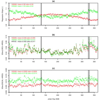
Fig. 5.Annual time series of(a)the linear regression slopes found to link variations in the HRV channel to unresolved variations in the 0.6 (VIS006, red) and 0.8 µm (VIS008, green) channel;(b)the es-timated standard deviation of the difference between 1×1 (HRES) and 3×3 km2(LRES) images for the three spectral channels; and of
(c)the estimated residual standard deviation of the proposed down-scaling algorithm. Periods when Meteosat-8 replaced Meteosat-9 as operational satellite due to spacecraft anomalies have been shaded in grey.
time series for the 0.6, 0.8 µm and HRV channels. The 0.6 and 0.8 µm values are estimated from the HRV values using the slopesS(r06)andS(r08), and applying the general
prop-erty of the variance thatVar(a x)=a2Var(x)for a constanta
and a random variablex. Panel Fig. 5c plots the time series of the expected residual standard deviation of the downscaled and true HRES images, based on the estimate of unresolved variability outlined in the previous paragraph.
Panel a of Fig. 5 shows that on average, the narrowband re-flectances of a HRES pixel within the 3×3 km2sampling res-olution of a LRES pixel deviates from the LRES reflectance by absolute amounts of 0.049 and 0.051 for the 0.6 and 0.8 µm images, respectively. This variability is not taken into account if only the LRES images are used. By applying our downscaling algorithm, we are able to reduce these devia-tions to values of only 0.007 and 0.011.
−0.4 −0.2 0.0 0.2 0.4 0.6 0.8 1.0
0
20
40
60
80
100
HRVIS Shift [km]
Counts [−]
Shift East Shift South
Mean: 0.36 km SDev: 0.11 km
Mean: 0.06 km SDev: 0.10 km
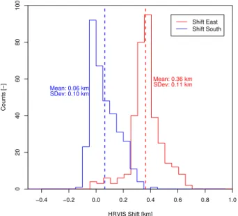
Fig. 6. Histogram of the shifts of the HRV image relative to the 0.6 and 0.8 µm channel in Northern and Eastern direction, obtained for 345 Meteosat-9 scenes from 2008. The shift of the images is expressed as distance at the nadir point of the satellite in kilometers (km).
is used. Four alternative filtering strategies have been tested to obtain LRES images from the HRV channel. Denoted by LP48, all Fourier coefficients above the Nyquist frequency (12×4.8−1km−1) were set to zero in the filtering process, cor-responding to a perfect lowpass filter for the 4.8×4.8 km2 resolution reported by Schmetz et al. (2002). An alternative is the use of arithmetic averaging of a neighborhood of pix-els. Here, square regions consisting of 1×1, 3×3 pixels and 5×5 pixels were considered. The values given in the table support that accounting for the functional form of the MTF does achieve the highest values of explained variance by a margin of at least 0.5%. The Fourier method used by the al-gorithm for image coregistration is able to detect and correct for shifts of the HRV images relative to the LRES images, and is not limited to integer multiples of the pixel resolution. Figure 6 shows histograms of the individual shift found, hav-ing a mean value of 0.06±0.10 in South and 0.36±0.11 km in East direction. These values indicate the good coregistration accuracy of the satellite images after EUMETSAT’s image rectification procedure. In consequence, not correcting for image misregistration reduces the correlation reported in Ta-ble 3 only slightly (NoCoReg). It can thus be argued that the additional complexity of coregistering the images is not worth the extra effort. For extreme cases, however, the shift can vary by more than half a HRV pixel, and the coregistra-tion procedure can then prevent a degradacoregistra-tion of accuracy.
5 Conclusions and outlook
In this paper, a downscaling algorithm is presented to en-hance the spatial resolution of Meteosat SEVIRI 0.6 and 0.8 µm narrowband images by a factor of 3. Our algorithm utilizes the broadband HRV channel in a linear model to re-solve the high-frequency spatial variability for the lower spa-tial resolution narrowband channels. In addition, the spaspa-tial response functions of the SEVIRI channels are accounted for by an explicit convolution with the sensor modulation trans-fer function and the Fourier shift theorem is used to coregis-ter the HRV broadband channel to the narrowband channels. The results of our uncertainty analysis reveal that our ap-proach resolves high-frequency variability in the narrowband channels with an explained variance of 98.2% and 95.3% in the 0.6 and 0.8 µm channels, respectively, corresponding to residual standard deviations of 0.007 and 0.011 for the downscaled narrowband reflectances. In comparison, aver-age values of 0.049 and 0.052 are expected as standard de-viation between the reflectance of a HRES and an enclosing LRES pixel, variability which is completely neglected in the lower resolution narrowband images. These numbers support that the algorithm is able to provide physically consistent 0.6 and 0.8 µm reflectance images at the spatial resolution of the HRV channel.
Two sources of uncertainty of the proposed algorithm have been identified. First, it is assumed that the reflectance of the HRV channel is a linear combination of the 0.6 and the 0.8 µm reflectance. Second, the accuracy of the inversion of this linear relation relies on the correlation between the 0.6 and 0.8 µm channel reflectance, and the ratio of their vari-ance. The latter uncertainty has been found to dominate, and is larger for the 0.8µm channel, as its contribution to the HRV reflectance is less than that of the 0.6 µm channel. This fact is also reflected by the lower value of explained variance of the downscaled 0.8 µm channel given above.
Two aspects relevant to the accuracy of the downscaling algorithm have been studied in this paper. First, the cor-respondence of spatial variations between the narrowband and downsampled HRV channels improves significantly if the modulation transfer function of the SEVIRI sensors is explicitly used in the downsampling procedure. Second, the coregistration of the HRV and narrowband channels has been quantified, and only a minor shift has been found of 0.06±0.10 and 0.36±0.11 km in South and East direction, respectively. Methods based on the discrete Fourier trans-form have been introduced to address both aspects.
forcing (Oreopoulos et al., 2009). Other applications, such as the early detection of convective activity and the retrieval of land surface properties, can likely also benefit from the enhanced spatial resolution of the narrowband channels.
The main limitation of the approach in its current form is the fact that only a single linear model is used to down-scale the entire SEVIRI scene. Since clouds dominate the spatial variations in reflectance (Deneke et al., 2009a) they also dominate the spectral variations and correlations in re-flectance, and thus the applicability of the linear model. The relationship between narrowband and broadband radiances is known to be dependent on scene type (Li and Leighton, 1992). The use of scene-dependent linear models, using a previous pixel classification, could be a promising algorithm extension. Another promising extension could be the use of external sources of information within the downscaling pro-cess. For example, MODIS products could provide some of the required statistical parameters at high-resolution, such as the correlation between the 0.6 and 0.8 µm channel.
The algorithm presented in this paper is a physical down-scaling method, which exploits the availability of higher spa-tial resolution information from the HRV channel as predic-tor (see Liu and Pu (2008) for the distinction between statis-tical and physical downscaling methods). The combination with statistical techniques could help extend the downscaling to additional SEVIRI spectral channels. It also needs consid-eration that the HRV channel is only available for part of the disk of the earth observed by SEVIRI, and that it still has a lower resolution than comparable polar-orbiting satellite im-agers. Moreover, Deneke et al. (2009b) showed that biases in satellite-estimated cloud climatologies can also be reduced by using estimates of the unresolved variance. Alternatively or complementary, these biases may also be reduced by us-ing approaches that simulate realistic surrogate variability at sub-pixel scale (see e.g., Venema et al., 2010; Schutgens and Roebeling, 2009).
Finally, our results demonstrate the potential of combining satellite images with different spatial and spectral resolution, to benefit from their individual strengths. This point will be-come even more important in the future for Meteosat Third Generation, which will acquire images with several different spatial resolutions.
Appendix A
Spectral channel characteristics
The following quantities are introduced to characterize the spectral response functionηof a satellite detector. ηis as-sumed to be normalized to a maximum value of unity here. The spectral widthδλof a channel is given by
δλ=
Z ∞
0
η(λ)dλ. (A1)
Then, the central wavelengthλCcan be defined as
λC=
1
δλ
Z ∞
0
λη(λ)dλ. (A2)
The band-averaged extraterrestrial solar spectral irradiance
φCof a channel is finally calculated by
φC=
1
δλ
Z ∞
0
φ (λ)η(λ)dλ. (A3)
Here,φ is the extraterrestrial solar spectrum at a sun-earth distance of 1 astronomical units.
The quantitiesλCandδλare well-suited to determine bulk
optical properties of a medium illuminated by a spectrally constant source of irradiance. In case of the earth’s atmo-sphere, however, the incident solar irradiance varies strongly with wavelength. It is therefore more appropriate to use the productη∗=ηφof spectral response and solar spectrum in-stead ofηto weight the reflection and transmission properties of the earth’s atmosphere and surface for a spectral interval. Replacingηwithη∗ in Eq. (A1) and Eq. (A2), analoguous
quantitiesλ∗
Candδλ∗can be obtained.
Appendix B
Statistical inversion
This appendix presents general statistical relations used by this paper, and applies them in order to invert Eq. (5). First, we consider a random variableywhich is assumed to be lin-early related to an independent variablesxby
y=a x+b. (B1)
Here,adenotes the slope andbthe offset of the linear model. Using standard definitions of variance and covariance, an es-timatebaof the slope of the linear relation is given by
ba=Cov(x,y)
Var(x) =Cor(x,y)
s Var(y)
Var(x), (B2)
which minimizes the sum of the squared deviations ofyfrom the linear equation. In the second equality, the linear correla-tion coefficient has been used, which is related to the covari-ance through
Cor(x,y)=√Cov(x,y)
Var(x)Var(y). (B3)
The standard deviationσyof the difference between modeled
and observed values can be calculated by
σy=
q
Var(y)1−Cor(x,y)2. (B4)
This equation also motivates the nameexplained variance
EV (x,y)for the square ofCor(x,y), as σx2
Var(y) specifies the
We now consider the downscaling problem discussed in this paper. Here,ydepends linearly on two random and cor-related variablesx1andx2without any offset
y=a x1+bx2. (B5)
We are interested in the inversion of this linear model, to estimatex1andx2 fromy. Eq. (B2) can provide the slope
S(x1)of the least-squares solution for predictingx1fromy.
Inserting Eq. (B5) into Eq. (B2), and simplyfing with general properties of covariance and variance, we obtain:
S(x1)=
Cov(x1,y)
Var(y)
= 1+kCor(x1,x2)
a1+k2+2kCor(x
1,x2)
, (B6)
withkgiven by
k=
s
a2Var(x
2)
b2Var(x
1)
. (B7)
As measure of the accuracy of this linear model, the ex-plained varianceEV (x1,y)ofx1givenyis used. We obtain
EV(y,x1)=
Cov(y,x1)2
Var(y)Var(x1)
= [1+kCor(x1,x2)]
2
1+k2+2kCor(x
1,x2)
. (B8)
These results show that both the slope and the explained vari-ance of the inversion depend only on the correlation ofx1and
x2, the slopesaandb, as well as the ratio of the variances of
x1andx2. To apply these general results to the purposes of
this paper,a,b,x1andx2have to be chosen appropriately.
Acknowledgements. The work of the first author has been funded through a EUMETSAT research fellowship. The authors would like to thank Wouter Greuell, Jan Fokke Meirink and Victor Venema for their helpful comments and suggestions on earlier versions of this manuscript. We also greatly appreciated the helpfull discussions with Marianne K¨onig, Knut Dammann (both from EUMETSAT) and Carsten Mannel (from VCS) on MSG navigation and the inter-channel co-registration.
Edited by: J. Quaas
References
Anuta, P.: Spatial registration of multispectral and multitemporal digital imagery Using fast Fourier transform techniques, IEEE T. Geosci. Electr., 8(4), 353–368, 1970.
Cros, S., Albuisson, M., and Wald, L.: Simulating Meteosat-7 broadband radiances using two visible channels of Meteosat-8, Sol. Energy, 80(3), 361–367, 2006.
Deneke, H., Feijt, A., Lammeren, A., and Simmer, C.: Valida-tion of a Physical Retrieval Scheme of Solar Surface Irradiances from Narrowband Satellite Radiances, J. Appl. Meteorol., 44(9), 1453–1466, 2005.
Deneke, H., Feijt, A., and Roebeling, R.: Estimating surface solar irradiance from METEOSAT SEVIRI-derived cloud properties, Remote Sens. Environ., 112, 3131–3141, 2008.
Deneke, H., Knap, W., and Simmer, C.: Multiresolution analysis of the temporal variance and correlation of transmittance and reflectance of an atmospheric column, J. Geophys. Res., 114, D17206, doi:10.1029/2008JD011680, 2009a.
Deneke, H., Roebeling, R., Wolters, E., Feijt, A., and Simmer, C.: On the Sensitivity of Satellite-Derived Cloud Properties To Sen-sor Resolution and Broken Clouds, in: Current problems in at-mospheric radiation: Proceedings of the International Radiation Symposium (IRS 2008), 1100, 376–379, 2009b.
D¨urr, B., Zelenka, A., M¨uller, R., and Philipona, R.: Ver-ification of CM-SAF and MeteoSwiss satellite based re-trievals of surface shortwave irradiance over the Alpine region, Int. J. Remote Sens., ISSN: 1366-5901 31(15), 4179–4198, doi:10.1080/01431160903199163, 2010.
EUMETSAT: SEVIRI Modulation Transfer Function (MTF) characterisations for MSG-1, MSG-2 and MSG-3, Tech. rep., EUMETSAT, Darmstadt, Germany, http://www.eumetsat. int/idcplg?IdcService=GET FILE&dDocName=ZIP MSG SEVIRI SPEC RES CHAR&RevisionSelectionMethod= LatestReleased, 2006a.
EUMETSAT: MSG SEVIRI spectral response charac-terization, Tech. rep., EUMETSAT, Darmstadt, Ger-many, http://www.eumetsat.int/idcplg?IdcService= GET FILE&dDocName=ZIP MSG MOD TRANSF FUN CHARS&RevisionSelectionMethod=LatestReleased, 2006b. Greuell, W. and Roebeling, R.: Towards a standard procedure for
validation of satellite-derived cloud liquid water path, J. Atmos. Sci., 48, 1575–1590, doi:10.1175/2009JAMC2112.1, 2009. Gueymard, C.: The Sun’s total and spectral irradiance for solar
energy applications and solar radiation models, Solar Energy, 76(4), 423–452, 2004.
Harris, F.: On the use of windows for harmonic analysis with the discrete Fourier transform, Proc. IEEE, 66(1), 51–83, 1978. Heidinger, A. and Stephens, G.: Molecular line absorption in a
scat-tering atmosphere. Part III: Pathlength characteristics and effects of spatially heterogeneous clouds, J. Atmos. Sci., 59(10), 1641– 1654, 2001.
Jacobowitz, H., Stowe, L., Ohring, G., Heidigner, A., Knapp, K., and Nalli, N.: The Advanced Very High Resolution Radiometer Pathfinder Atmosphere (PATMOS) climate dataset: a resource for climate research, B. Am. Meteorol. Soc., 84, 785–793, 2003. Kl¨user, L., Rosenfeld, D., Macke, A., and Holzer-Popp, T.: Obser-vations of shallow convective clouds generated by solar heating of dark smoke plumes, Atmos. Chem. Phys., 8(10), 2833–2840, doi:10.5194/acp-8-2833-2008, 2008.
Knap, W., Stammes, P., and Koelemeijer, R.: Cloud thermodynamic phase determination from near-infrared spectra of reflected sun-light, J. Atmos. Sci., 59(1), 83–96, 2002.
Lensky, I. and Rosenfeld, D.: Clouds-aerosols-precipitation anal-ysis tool (CAPSAT), Atmos. Chem. Phys., 8, 6739–6753, doi:10.5194/acp-8-6739-2008, 2008.
Liu, D. and Pu, R.: Downscaling thermal infrared radiance for sub-pixel land surface temperature retrieval, Sensors, 8(4), 2695– 2706, 2008.
Markham, B.: The Landsat sensor’s spatial response, IEEE T. Geosci. Remote Sens., GE-23(6), 864–875, 1985.
M¨uller, R., Matsoukas, C., Gratzki, A., Behr, H., and Hollmann, R.: The CM-SAF operational scheme for the satellite based retrieval of solar surface irradiance – A LUT based eigenvector hybrid approach, Remote Sens. Environ., 113(5), 1012–1024, 2009. Oreopoulos, L. and Davies, R.: Plane parallel albedo biases from
satellite observations. Part I: Dependence on resolution and other factors, J. Climate, 11, 919–932, 1998.
Oreopoulos, L., Platnick, S., Hong, G., Yang, P., and Cahalan, R. F.: The shortwave radiative forcing bias of liquid and ice clouds from MODIS observations, Atmos. Chem. Phys., 9, 5865–5875, doi:10.5194/acp-9-5865-2009, 2009.
Platnick, S., King, M., Ackerman, S., Menzel, W., Baum, B., Riedi, J., and Frey, R.: The MODIS cloud products: algorithms and ex-amples from Terra, IEEE T. Geosci. Remote Sens., 44(2), 459– 473, 2003.
Roebeling, R. and van Meijgaard, E.: Evaluation of the daylight cycle of model predicted cloud amount and condensed water path over Europe with observations from MSG-SEVIRI, J. Climate, 22, 1749–1766, 2008.
Roebeling, R., Deneke, H., and Feijt, A.: Validation of cloud liquid water path retrievals from SEVIRI using one year of CloudNET observations, J. Appl. Meteorol., 47(1), 206–222, 2008. Rossow, W. and Schiffer, R.: ISCCP cloud data products, B. Am.
Meteorol. Soc., 71, 2–20, 1991.
Schmetz, J., Mhita, M., and van den Berg, L.: METEOSAT Obser-vations of Longwave Cloud-Radiative Forcing for April 1985, J. Climate, 3, 784–791, 1990.
Schmetz, J., Pili, P., Tjemkes, S., Just, D., Kerkmann, J., Rota, S., and Ratier, A.: An introduction to Meteosat Second Generation (MSG), B. Am. Meteorol. Soc., 83, 977–992, 2002.
Schulz, J., Albert, P., Behr, H.-D., Caprion, D., Deneke, H., De-witte, S., D¨urr, B., Fuchs, P., Gratzki, A., Hechler, P., Holl-mann, R., Johnston, S., Karlsson, K.-G., Manninen, T., M¨uller, R., Reuter, M., Riihel¨a, A., Roebeling, R., Selbach, N., Tetzlaff, A., Thomas, W., Werscheck, M., Wolters, E., and Zelenka, A.: Operational climate monitoring from space: the EUMETSAT satellite application facility on climate monitoring (CM-SAF), Atmos. Chem. Phys., 9(5), 1687–1709, doi:10.5194/acp-9-1687-2009, 2009.
Schutgens, N. A. J. and Roebeling, R. A.: Validating the Validation: The Influence of Liquid Water Distribution in Clouds on the Intercomparison of Satellite and Surface Observations. J. Atmos. Ocean. Technol., 26, 1457–1474, doi:10.1175/2009JTECHA1226.1, 2009.
Stephens, G. and Kummerow, C.: The remote sensing of clouds and precipitation from space: a review, J. Atmos. Sci., 64, 3742– 3765, 2007.
Venema, V., Garcia, S., and Simmer, C.: A new algorithm for the downscaling of 3-dimensional cloud fields, Q. J. Roy. Meteorol. Soc., 136(646), 91–106, doi:10.1002/qj.535, 2010.
Walker, P. and Mallawaarachchi, T.: Disaggregating agricultural statistics Using NOAA-AVHRR NDVI – a variant of the tradi-tional spatial problem, Remote Sens. Environ., 63(2), 112–125, 1998.
Wielicki, B., Barkstrom, B., Harrison, E., III, R. L., Smith, G., and Cooper, J.: Clouds and the Earth’s Radiant Energy System (CERES): An Earth Observing System experiment, B. Am. Me-teorol. Soc., 77(5), 853–868, 1995.
Wolters, E., Deneke, H., van den Hurk, B., Meirink, J. F., and Roe-beling, R.: Broken and inhomogeneous cloud impact on satellite cloud particle effective radius and cloud-phase retrievals, J. Geo-phys. Res., 115, D10214, doi:10.1029/2009JD012205, 2010. Woods, J., Barkmann, W., and Horch, A.: Solar heating of the