Study of final-state radiation in decays of Z bosons produced in pp collisions at 7 TeV

Study of final-state radiation in decays of

Z

bosons produced

in

pp

collisions at 7 TeV

V. Khachatryan et al.*

(CMS Collaboration)

(Received 27 February 2015; published 29 May 2015)

The differential cross sections for the production of photons in Z→μþμ−_γdecays are presented as a

function of the transverse energy of the photon and its separation from the nearest muon. The data for these measurements are collected with the CMS detector and correspond to an integrated luminosity of4_.7_fb−1

of pp collisions at ffiffiffi

s

p

¼7_{TeV delivered by the CERN LHC. The cross sections are compared to}

simulations withPOWHEGandPYTHIA, wherePYTHIAis used to simulate parton showers and final-state

photons. These simulations match the data to better than 5%.

DOI:10.1103/PhysRevD.91.092012 PACS numbers: 14.70.Hp, 12.38.-t, 13.40.Ks

I. INTRODUCTION

We present a study and differential cross section mea-surements of photons emitted in decays of Z bosons produced at a hadron collider. Such radiative decays of the Z boson were noted in the very first Z boson publications of UA1 and UA2[1,2], but subsequently have not been given a detailed study in hadron colliders. In 2011, the CERN LHC delivered ppcollisions at ffiffiffi

s p

¼7_TeV, and data corresponding to an integrated luminosity of 4.7fb−1were collected with the CMS detector. From these data, we select a sample of events in which a Z boson decays to aμþμ−pair and an energetic photon. We measure the differential cross sections dσ=dE_T with respect to the photon transverse energyE_Tanddσ=dΔRμγwith respect to

the separation of the photon from the nearest muon. Here,

ΔRμγ¼

ffiffiffiffiffiffiffiffiffiffiffiffiffiffiffiffiffiffiffiffiffiffiffiffiffiffiffiffiffiffiffiffiffiffiffiffiffiffiffiffiffiffiffiffiffiffiffi

ðϕμ−ϕγÞ2þ ðημ−ηγÞ2 q

, whereϕis the azimu-thal angle (in radians) around the beam axis andη is the pseudorapidity. The cross sections include contributions from the Z resonance, virtual photon exchange, and their interference, collectively referred to as Drell-Yan (DY) production.

Photons emitted in Z boson decays, which we call final-state radiation (FSR) photons, can be energetic (tens of GeV) and well separated from the leptons (by more than a radian). Quantum electrodynamics (QED) corrections that describe FSR production are well understood. Quantum chromodynamics (QCD) corrections modify the kinematic distributions of the Z boson; in particular, the Z boson acquires a nonzero component of momentum transverse to the beam:qT>0. TheFEWZprogram calculates both QCD

and QED corrections for the DY process [3]. However, it

does not include mixed QCD and QED corrections; the required two-loop integrals are technically very challeng-ing, and progress has been made only recently [4]. In practice, event generators employing matrix element cal-culations matched to parton showers must be used[5,6]. It is the goal of this analysis to establish the quality of the modeling of FSR over a wide kinematic and angular range. The results will support future measurements of the W mass, the study of Zþγ production, and searches for new particles in final states with photons.

In an attempt to compare photons emitted close to a muon (a process that is modeled primarily by a partonic photon shower) and far from the muons (which requires a matrix element calculation), we measure dσ=dET for

0_.05_<ΔR

μγ ≤0.5 and 0.5<ΔRμγ ≤3. Furthermore,

since the size of the QCD corrections varies with the transverse momentum of the Z boson, we measuredσ=dET

anddσ=dΔRμγforqT<10GeV andqT>50GeV, where

q_Tis defined as the vector sum of the transverse momenta of the two muons and the photon. These cross sections are defined with respect to the fiducial and kinematic requirements detailed below; no acceptance corrections are applied. Nonetheless, we do correct for detector resolution and efficiencies.

This article is structured as follows. We briefly describe the CMS detector and the event samples we use in Sec.II. The details of the event selection are given in Sec. III. Background estimation and the way we unfold the data distributions are discussed in Secs.IVandV. We discuss the systematic uncertainties in Sec.VI and report our results and summarize the work in Secs.VII andVIII.

II. THE CMS DETECTOR AND EVENT SAMPLES

A full description of the CMS detector can be found in Ref. [7]; here we briefly describe the components most important for this analysis. The central feature of the CMS experiment is a superconducting solenoid that provides an

*_{Full author list given at the end of the article.}

axial magnetic field of 3.8 T. A tracking system composed of a silicon pixel detector and a silicon strip detector is installed around the beam line, and provides measurements of the trajectory of charged particles for jη_j<2_.5_{. After} passing through the tracker, particles strike the crystal electromagnetic calorimeter (ECAL) followed by the brass and scintillator hadron calorimeter. The solenoid coil encloses the tracker and the calorimetry. Four stations of muon detectors measure the trajectories of muons that pass through the tracker and the calorimeters forjη_j<2_.4_{. Three} detector technologies are employed in the muon system: drift tubes for central rapidities, cathode strip detectors for the forward rapidities, and resistive-plate chambers for all rapidities. Combining information from the muon detectors and the tracker, the transverse momentum (pT) resolution

for muons used in this analysis varies from 1% to 6%, depending on η and pT [8]. The ET of photons and

electrons is measured using energy deposited in the ECAL, which consists of nearly 76 000 lead tungstate crystals distributed in the barrel region (_jη_j<1.479) and two end cap regions (1.479_<jηj<3.0). The photon energy resolution is better than 5% for the range of E_T pertinent to this analysis [9]. Events are selected using a two-level trigger system. The level-1 trigger composed of custom-designed processing hardware selects events of interest based on information from the muon detectors and calorimeters [10]. The high-level trigger is software based, running a simpler and therefore faster version of the off-line reconstruction code on the full detector informa-tion, including the tracker[11].

Simulated data samples are used to design and verify the principles of the analysis. They are also used to assess efficiencies, resolution, and backgrounds. The signal proc-ess is simulated using the POWHEG (V1.0) [12] event

generator with PYTHIA (V6.4.24) [13] used to simulate

parton showers and final-state photons (referred to in what follows as POWHEGþPYTHIA). This combination is also used for t¯_{t and diboson (WW, WZ, ZZ) production.} The CT10[14]parton distribution functions are used. The Z2 parameter set[15]is used to model the underlying event inPYTHIA, and the effects of additionalppcollisions that produce signals registered together with the main inter-action are included in the simulation.

The response of the detector is simulated using GEANT4 [16]. The simulated events are processed using the same version of the off-line reconstruction code used for the data.

III. EVENT SELECTION

The data are recorded using a trigger that requires two muons. One muon is required to have pT>13GeV, and

the other,pT>8GeV. This trigger has no requirement on

the isolation of the muons.

Events with a pair of oppositely charged, well-reconstructed, and isolated muons and an isolated photon are selected. The kinematic and fiducial requirements for

selecting events are based wholly on the muon and photon kinematic quantities, and are summarized in Table I. As explained below, we use the dimuon massMμμto define a “signal region”that is rich in FSR photons, and a“control

region”that is dominated by background sources of photons.

Muons are selected in the manner developed for the measurements of the DY cross section[17]. They must be reconstructed using an algorithm that finds a track segment in the muon detectors and links it with a track in the silicon tracker, and also through an algorithm that extrapolates a track in the silicon tracker outward and matches it with hits registered in the muon detectors. We select the two highest pT muons (which we will call “leading” and “trailing”),

and ignore any additional muons. These two muons must have opposite charge. The leading muon must satisfy the requirementspT>31GeV andjηj<2.4, while the

trail-ing muon must satisfyp_T>9_{GeV andjηj<}2_.4_{to ensure} good reconstruction efficiency. A vertex fit is performed to the two muon tracks, and theχ2_{probability of the fit must}

be at least 0.02. We define the difference betweenπand the opening angle of the two muons as the acollinearityα, and remove a very small region of phase space whereαis less than 5 mrad to reduce contamination by cosmic rays to a negligible level.

Photons are reconstructed using the particle flow (PF) algorithm [18,19] that uses clustered energy deposits in ECAL. The PF algorithm allows us to reconstruct photons at relatively low ET and to maintain coherence with the

calculation of the isolation observables described below. Photons that convert to electron-positron pairs are included in this reconstruction. Events selected for this analysis must have at least one photon withE_T>5_{GeV, and the} separation of this photon with respect to the closest muon must satisfy0_.05_<ΔR

μγ ≤3. Studies using the simulation

show that photons with ΔRμγ <0.05 are difficult to

reconstruct reliably due to the energy deposition left by the muon, and no signal photons with ΔRμγ >3 are

expected. If an event has more than one photon satisfying this selection criteria, we select the one with the highestET.

In events in which one photon is selected, a second photon is present 15% of the time; however, these extra photons are expected to be mostly background, since the fraction of TABLE I. Summary of kinematic and fiducial event require-ments.

Object Requirement

Leading muon p_T>31_{GeV and jηj<}2_.4

Trailing muon p_T>9_{GeV andjηj}<2_.4

Acollinearity α>0_.005_radians

Photon E_T>5_GeV,jηj<2_.4_{but not}

1_.4_<jηj<1_.6_;0_.05_<ΔRμγ≤3

Signal region 30_{< Mμμ<}87_GeV

events with a second FSR photon in simulation is approx-imately 0.5%. More details about these background pho-tons are given in Sec. IV.

All three particles emitted in the Z boson decay—the two

muons and the photon—_{are usually isolated from other}

particles produced in the same bunch crossing. We can reduce backgrounds substantially by imposing appropriate isolation requirements. The isolation quantities,Iμfor the

muons and Iγ for the photon, are based on the scalar pT

sums of reconstructed PF particles within a cone around the muon or photon direction. The cone size for both muons and photons isΔR_¼0.3. The muon_pTis not included in the sum for Iμ, and the photon ET is not included in the

sum forIγ; these isolation quantities are meant to represent

the energy carried by particles originating from the main primary vertex close to the given muon or photon. For a well-isolated muon or photon,Iμ orIγ should be small.

Special care is taken to avoid inefficiencies and biases occurring when the FSR photon falls close to the muon; in such cases the muon and the photon may appear, super-ficially, to be nonisolated. To avoid this effect, we exclude any PF photon from the muon isolation sum. Furthermore, since the photon can convert and produce charged particle tracks that cannot always be unambiguously identified as an eþe− pair, we exclude from the muon isolation sum charged tracks that lack hits in the pixel detector or that have pT<0.5GeV. Finally, any particle that lands in a

cone ofΔR <0.2around a PF photon is excluded from the muon isolation sum. After these modifications to the muon isolation variable, the efficiency of the isolation require-ment is flat (98%) for all ΔRμγ and is higher than the

efficiency of the unmodified isolation requirement by about 0.5%. Adding these modifications does not significantly increase the backgrounds.

The instantaneous luminosity of the LHC was suffi-ciently high that each bunch crossing resulted in multiple pp collisions (8.2 on average). The extraneouspp colli-sions are referred to as “_pileup” _{and must be taken into}

consideration when defining and calculating the muon and photon isolation variables. Charged hadrons, electrons, and muons coming from pileup can be identified by checking their point of origin along the beam line, which will typically not coincide with the primary vertex from which the muons originate. When summing the contributions of charged hadrons, electrons, and muons to the isolation variable, those coming from pileup are excluded. This distinction is not possible for photons and neutral hadrons, however. Instead, an estimate Ip of the contribution of

photons and neutral hadrons to the sum is made: we use one-half of the (already excluded) contribution from charged hadrons within the isolation cone. This estimate is subtracted from the sum of contributions from photons and neutral hadrons; if the result is negative, we then use a net contribution of zero.

We designate byI_h the sum ofp_Tfor charged particles that are not excluded from the isolation sum. We letIemand

Ih0stand for the sums over thep_Tof all photons and neutral hadrons, andIpfor the estimate of the pileup contribution

toIem andIh0. The muon isolation variable is, then,

Iμ¼ ðIhþI_h0Þ=p_T: ð1Þ

Note that the sum is normalized to thepTof the muon. We

requireIμ<0.2 for both muons.

The photon isolation variable is calculated as above, except that the muons are not included in the sum, and there is no special exclusion of charged tracks near the photon:

Iγ ¼IhþmaxðI_emþI_h0₋I_p;0Þ: ð2Þ

We requireIγ <6GeV.

The emission of FSR photons in Z boson decays reduces the momenta of the muons. Consequently, the dimuon mass Mμμtends to be lower thanMZ, the nominal mass of the Z boson. Simulations indicate that, for most of the signal, Mμμ<87GeV, due to the requirement ET>5GeV for

the photon. They also show that theMμμ distribution for

radiative decays Z→μþμ−_γ ends at M

μμ≈30GeV. A

requirementMμμ >30GeV also helps to avoid a kinematic

region in which the acceptance is difficult to model. Therefore, our signal region is defined by

30_{< Mμμ <}87GeV. We also define a control region by

89_{< M}

μμ <100GeV, where the contribution of FSR

photons is quite small (below 0.5%). The numbers of events we select are 56 005 in the signal region and 45 277 in the control region.

IV. BACKGROUND ESTIMATION

Nearly all selected events have two prompt muons from the DY process. Backgrounds come mainly from “

non-prompt”photons, which may be genuine photons produced

in the decays of light mesons (such asπ0_and

η), a pair of overlapping photons that cannot be distinguished from a single photon, and photons from pileup. We study these backgrounds with simulated DY events and apply correc-tions so that the simulation reproduces the data distribu-tions, as described in detail below.

Some events come from processes other than DY, such as t¯_{t and diboson production. These backgrounds are} very small and are estimated using the simulation. Similarly, a small background from the DY production ofτþτ−is also estimated from simulation. The background from multijet events, including events with a W_→μν

The control region is dominated by nonprompt photons whose kinematic distributions (ET, η, ΔRμγ) are nearly

identical to nonprompt photons in the signal region. Quantitative comparisons of data and simulation revealed significant discrepancies in the control region that prompted corrections to the simulation, which we now explain.

The POWHEGþPYTHIA sample does not reproduce the number of jets per event well, so we apply weights to the simulated events as a function of the number of reconstructed jets in each event. For this purpose, jets are reconstructed from PF objects using the anti-kTalgorithm [20]with a size parameterR¼0_.5_{. We consider jets with} pT>20GeV and jηj<2.4 that do not overlap with the

muons or the photon.

Studies ofIγfor events in the control region reveal small

discrepancies in the multiplicity andpTspectra of charged

hadrons included in the sum. We apply weights to the simulated events to bring the multiplicities into agreement, and we impose pT>0.5GeV on charged hadrons. The

simulatedIγ distributions match those in the data very well

after applying these weights.

Finally, theETandηdistributions of nonprompt photons

in the simulation deviate from those in the data. We fit simple analytic functions to the ratios of the data to simulated E_T and η distributions and define a weight as the product of those functions. We check that this factori-zation is valid (i.e., that theET correction is the same for

different narrow ranges ofη, and vice versa).

After these three corrections (for jet multiplicity, for the spectrum of charged hadrons in the isolation sums, and for the ET and η of the nonprompt photon), the simulation

matches the data in all kinematic distributions in the control region, an example of which is shown in Fig.1, top. The total change in the background estimate due to these corrections is approximately 5% to 10%. We use the simulation with these weights to model the small back-ground in the signal region (Fig.1, bottom).

Given the definition of the signal region, the contribution of photons emitted in the initial state is very small (on the order of 4_×10−4 as determined from the POWHEGþ PYTHIA sample) and is counted as signal.

V. CORRECTING FOR DETECTOR EFFECTS

Our goal is to measure differential cross sections in a form that is optimal for testing FSR calculations. Therefore we are obliged to remove the effects of detector resolution and efficiency (including reconstruction, isolation, and trigger efficiency). The corrections for the muons follow the techniques developed for the DY cross section mea-surements [17]. The corrections for photons are applied using an unfolding technique, as discussed in this section. We apply small corrections to the muon momentum scale as a function of muonpT,ημ, andϕμ[21]; they have almost

no impact on our measurements. The muon reconstruction TABLE II. Composition of the signal sample. The simulation

has been tuned to reproduce the data in the control region.

Process Fraction

Signal 77.1%

DY with a nonprompt photon 9.5%

Pileup 11.2%

t¯_{t 0.6%}

τþτ− 0.3%

Dibosons 0.2%

Multijets 1.1%

) [GeV]

γ

Photon Isolation (I

0 2 4 6 8 10 12 14

Events

2

10

3

10

4

10

5

10 Data

FSR

Underlying event and nonprompt Pileup

Non-DY background

< 100 [GeV]

μ μ

89 < M

(7 TeV) -1 4.7 fb

CMS

) [GeV]

γ

Photon Isolation (I

0 2 4 6 8 10 12 14

Data/MC 0.8

1 1.2

) [GeV]

γ

Photon Isolation (I

0 2 4 6 8 10 12 14

Events

2

10

3

10

4

10

5

10

Data FSR

Underlying event and nonprompt Pileup

Non-DY background

< 87 [GeV]

μ μ

30 < M

(7 TeV) -1 4.7 fb

CMS

) [GeV]

γ

Photon Isolation (I

0 2 4 6 8 10 12 14

Data/MC 0.8

1 1.2

FIG. 1 (color online). Distributions of the photon isolation variableIγ for the control region (top) and for the signal region

TABLE III. Relative systematic uncertainties fordσ=dE_T (in percent).

Kinematic requirement (GeV)

Background estimation

Muon efficiency

PhotonE_T scale

Photon E_T resolution

Photon efficiency

Pileup

photons Unfolding Total

0_.05<_ΔR_μγ≤3

5< E_T≤10 _{2.7 3.0 0.5 1.0 2.0 1.5 1.4 5.1}

10_{< ET}≤15 _{1.3 2.5 0.5 0.5 1.0 0.4 1.4 3.4}

15< E_T≤20 _{0.9 2.5 0.5 0.5 1.3 0.1 1.4 3.3}

20_{< ET}≤25 _{0.8 2.7 0.5 0.5 1.4 <}0_.1 _{1.4 3.5}

25< E_T≤30 _{0.7 3.3 0.5 0.5 1.5} <0_.1 _{1.4 4.0}

30_{< ET}≤40 _{1.0 4.3 0.5 0.5 1.1 0.1 1.4 4.8}

40< E_T≤50 _{2.9 4.4 1.0 0.5 2.8 0.5 1.4 6.3}

50_{< ET}≤75 _{7.2 4.5 1.0 0.5 2.0 0.6 1.4 8.9}

75< E_T≤100 _{15.3 4.5 3.0 1.0 6.9 1.1 1.4 17.8}

0_.05_<ΔRμγ≤0_.5

5< E_T≤10 _{0.8 2.1 0.5 1.0 2.0 0.1 1.4 3.5}

10_{< ET}≤15 _{0.4 2.0 0.5 0.5 1.0 <}0_.1 _{1.4 2.8}

15< E_T≤20 _{0.3 2.2 0.5 0.5 1.3} <0_.1 _{1.4 3.1}

20_{< ET}≤25 _{0.3 2.5 0.5 0.5 1.4 <}0_.1 _{1.4 3.3}

25< E_T≤30 _{0.2 3.2 0.5 0.5 1.5} <0_.1 _{1.4 3.9}

30_{< ET}≤40 _{0.3 4.3 0.5 0.5 1.1 <}0_.1 _{1.4 4.7}

40< E_T≤50 _{0.9 3.9 1.0 0.5 2.8} <0_.1 _{1.4 5.2}

50_{< ET}≤75 _{2.3 3.0 1.0 0.5 2.0 <}0_.1 _{1.4 4.6}

75< E_T≤100 _{4.9 3.1 3.0 1.0 6.9 0.8 1.4 9.7}

0_.5_<ΔRμγ ≤3

5_{< ET}≤10 _{6.4 4.7 0.5 1.0 2.0 3.8 1.4 9.2}

10< E_T≤15 _{2.8 3.2 0.5 0.5 1.0 0.8 1.4 4.7}

15_{< ET}≤20 _{1.9 2.8 0.5 0.5 1.3 0.3 1.4 4.0}

20< E_T≤25 _{1.7 3.0 0.5 0.5 1.4} <0_.1 _{1.4 4.0}

25_{< ET}≤30 _{1.6 3.4 0.5 0.5 1.5 0.1 1.4 4.3}

30< E_T≤40 _{2.3 4.4 0.5 0.5 1.1 0.2 1.4 5.3}

40_{< ET}≤50 _{6.5 5.1 1.0 0.5 2.8 1.3 1.4 9.0}

50< E_T≤75 _{16.1 8.1 1.0 0.5 2.0 2.0 1.4 18.4}

75_{< ET}≤100 _{34.5 6.2 3.0 1.0 6.9 3.5 1.4 36.0}

0_.05<_ΔR_μγ ≤3 _andq_T<10_GeV

5_{< ET}≤10 _{1.4 2.2 0.5 1.0 2.0 1.0 1.4 3.9}

10< E_T≤15 _{0.6 1.9 0.5 0.5 1.0 0.1 1.4 2.8}

15_{< ET}≤20 _{0.4 2.1 0.5 0.5 1.3 <}0_.1 _{1.4 3.0}

20< E_T≤25 _{0.4 2.4 0.5 0.5 1.4} <0_.1 _{1.4 3.3}

25_{< ET}≤30 _{0.5 3.5 0.5 0.5 1.5 <}0_.1 _{1.4 4.1}

30< E_T≤40 _{0.6 5.1 0.5 0.5 1.1} <0_.1 _{1.4 5.5}

40_{< ET}≤50 _{7.3 4.7 1.0 0.5 2.8 1.0 1.4 9.4}

50< E_T≤75 _{18.2 8.5 1.0 0.5 2.0 4.4 1.4 20.8}

75_{< ET}≤100 _{38.9 6.4 3.0 1.0 6.9 <}0_.1 _{1.4 40.2}

0_.05<_ΔR_μγ ≤3 _andq_T>50_GeV

5< E_T≤10 _{5.7 4.2 0.5 1.0 2.0 1.8 1.4 7.8}

10_{< ET}≤15 _{3.0 3.3 0.5 0.5 1.0 0.4 1.4 4.9}

15< E_T≤20 _{3.0 2.8 0.5 0.5 1.3 0.3 1.4 4.6}

20_{< ET}≤25 _{2.3 2.7 0.5 0.5 1.4 0.2 1.4 4.2}

25< E_T≤30 _{1.9 2.6 0.5 0.5 1.5 0.1 1.4 3.9}

30_{< ET}≤40 _{2.9 2.9 0.5 0.5 1.1 0.3 1.4 4.6}

40< E_T≤50 _{1.5 2.8 1.0 0.5 2.8 0.2 1.4 4.6}

50_{< ET}≤75 _{3.9 2.8 1.0 0.5 2.0 0.3 1.4 5.5}

efficiency (taken from simulation and corrected to match the data as a function ofpTandημ) is taken into account by

applying weights on a per-event basis. We do not correct for the approximately 0.5% increase in the isolation efficiency coming from the way we handle FSR photons falling within the muon isolation cone.

The energy scale and efficiencies for photons are more central to our task. Most PF photon energies correspond to the true energies within a few percent. However, in about 13% of the cases the photon energy is significantly underestimated. The simulation reproduces this effect very well. We construct a“_response”_{matrix that relates the PF}

energy to the true energy as a function ofηγ andΔRμγ. The

angular quantities ηγ andΔRμγ are themselves well

mea-sured. We use the iterative D’_{Agostini method of unfolding} [22]as implemented in the ROOUNFOLDpackage[23]. By

default, we unfold in the three quantitiesET,ηγ, andΔRμγ

simultaneously after subtracting backgrounds; as a cross-check we also unfold theETandΔRμγdistributions one at a

time, and we also use a single-value decomposition method

[24]. All results are consistent with each other. To verify the independence of the unfolded result on the assumed spectra, we distort the FSR model in an arbitrary manner when reconstructing the response matrix. The unfolded result is no different than the original one we obtained. A closure test in which the simulation is treated as data and undergoes the same unfolding procedure indicates no deviation greater than 1.5%.

The unfolding procedure corrects for the photon reconstruction and isolation efficiency. It also corrects for bias in the PF photon energy assuming that such a bias is reproduced in the simulation. Verification of the photon efficiencies and energy scale in the data with respect to the simulation are discussed in Sec.VI.

VI. SYSTEMATIC UNCERTAINTIES

Systematic uncertainties are assigned to each step of the analysis procedure using methods detailed in this section.

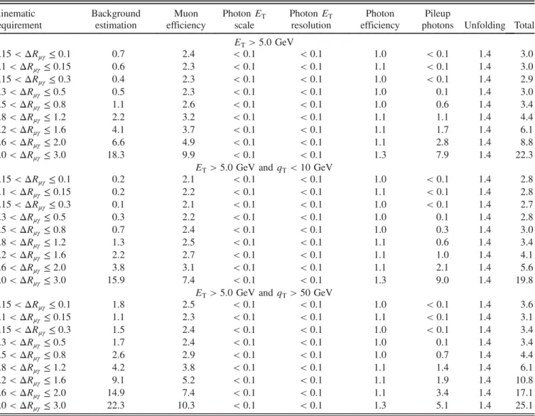
TABLE IV. Relative systematic uncertainties fordσ=dΔRμγ (in percent).

Kinematic requirement

Background estimation

Muon efficiency

PhotonE_T scale

PhotonE_T resolution

Photon efficiency

Pileup

photons Unfolding Total

E_T>5_.0_GeV

0_.15_<ΔRμγ ≤0_.1 _{0.7 2.4 <}0_.1 _<0_.1 _{1.0 <}0_.1 _{1.4 3.0} 0_.1_<ΔRμγ≤0_.15 _{0.6 2.3 <}0_.1 _<0_.1 _{1.1 <}0_.1 _{1.4 3.0} 0_.15<_ΔR_μγ ≤0_.3 _{0.4 2.3} <0_.1 <0_.1 _1.0 <0_.1 _{1.4 2.9}

0_.3<_ΔRμγ≤0.5 0.5 2.3 <0.1 <0.1 1.0 0.1 1.4 3.0

0_.5_<ΔRμγ≤0_.8 _{1.1 2.6 <}0_.1 _<0_.1 _{1.0 0.6 1.4 3.4}

0_.8_<ΔRμγ≤1_.2 _{2.2 3.2 <}0_.1 _<0_.1 _{1.1 1.1 1.4 4.4}

1_.2_<ΔRμγ≤1_.6 _{4.1 3.7 <}0_.1 _<0_.1 _{1.1 1.7 1.4 6.1}

1_.6<_ΔRμγ≤2.0 6.6 4.9 <0.1 <0.1 1.1 2.8 1.4 8.8

2_.0_<ΔRμγ≤3_.0 _{18.3 9.9 <}0_.1 _<0_.1 _{1.3 7.9 1.4 22.3}

E_T>5_.0_{GeV andqT<}10_GeV

0_.15<_ΔR_μγ ≤0_.1 _{0.2 2.1} <0_.1 <0_.1 _1.0 <0_.1 _{1.4 2.8} 0_.1_<ΔRμγ≤0_.15 _{0.2 2.2 <}0_.1 _<0_.1 _{1.1 <}0_.1 _{1.4 2.8} 0_.15_<ΔRμγ ≤0_.3 _{0.1 2.1 <}0_.1 _<0_.1 _{1.0 <}0_.1 _{1.4 2.7}

0_.3_<ΔRμγ≤0_.5 _{0.3 2.2 <}0_.1 _<0_.1 _{1.0 0.1 1.4 2.8}

0_.5<_ΔR_μγ≤0_.8 _{0.7 2.4} <0_.1 <0_.1 _{1.0 0.3 1.4 3.0}

0_.8_<ΔRμγ≤1_.2 _{1.3 2.5 <}0_.1 _<0_.1 _{1.1 0.6 1.4 3.4}

1_.2_<ΔRμγ≤1_.6 _{2.2 2.7 <}0_.1 _<0_.1 _{1.1 1.0 1.4 4.1}

1_.6_<ΔRμγ≤2_.0 _{3.8 3.1 <}0_.1 _<0_.1 _{1.1 2.1 1.4 5.6}

2_.0<_ΔR_μγ≤3_.0 _{15.9 7.4} <0_.1 <0_.1 _{1.3 9.0 1.4 19.8}

E_T>5.0GeV andq_T>50GeV

0_.15_<ΔRμγ ≤0_.1 _{1.8 2.5 <}0_.1 _<0_.1 _{1.0 <}0_.1 _{1.4 3.6} 0_.1<_ΔR_μγ≤0_.15 _{1.1 2.3} <0_.1 <0_.1 _1.1 <0_.1 _{1.4 3.1} 0.15<_ΔRμγ ≤0.3 1.5 2.4 <0.1 <0.1 1.0 <0.1 1.4 3.4

0_.3_<ΔRμγ≤0_.5 _{1.7 2.4 <}0_.1 _<0_.1 _{1.0 0.1 1.4 3.4}

0_.5_<ΔRμγ≤0_.8 _{2.6 2.9 <}0_.1 _<0_.1 _{1.0 0.7 1.4 4.4}

0_.8<_ΔR_μγ≤1_.2 _{4.2 3.8} <0_.1 <0_.1 _{1.1 1.4 1.4 6.1}

1.2<_ΔRμγ≤1.6 9.1 5.2 <0.1 <0.1 1.1 1.9 1.4 10.8

1_.6_<ΔRμγ≤2_.0 _{14.9 7.4 <}0_.1 _<0_.1 _{1.1 3.4 1.4 17.1}

Tables IIIandIVpresent a summary of these uncertain-ties, which are similar in magnitude to, or somewhat larger than the statistical uncertainties, depending on the photonET.

The muon efficiency taken from simulation is corrected as a function ofpTandηusing a method derived from the

data and described in Ref.[17]. The statistical uncertainties for these corrections constitute a systematic uncertainty, which we also take from Ref.[17]. In addition, we assign a 0.5% uncertainty to account for the modifications of the standard isolation variable. We propagate the uncertainty in the muon efficiency by shifting the per-event weights up and down by one unit of systematic uncertainty.

The photonETscale is potentially an important source of

systematic uncertainty although simulations indicate that

the bias in PF photon energy is negligibly small. We verify the fidelity of the simulation by introducing an extra requirement, 0_.05_<ΔR

μγ ≤0.9, which gives us a

high-purity subset of signal events in which the energy of the photon can be estimated from just the muon kinematics. We

s

-1 -0.8 -0.6 -0.4 -0.2 0 0.2 0.4 0.6 0.8 1

Events / (0.05)

0 200 400 600 800 Data MC Data fit MC fit (7 TeV) -1 4.7 fb

CMS

5 < E

s

-1 -0.8 -0.6 -0.4 -0.2 0 0.2 0.4 0.6 0.8 1

Events / (0.05)

0 50 100 150 200 250 Data MC Data fit MC fit (7 TeV) -1 4.7 fb

CMS

ECAL End cap

< 40 [GeV] T

20 < E

FIG. 2 (color online). Two examples of an sdistributions¼

1_−ðM2

μμγ−M 2

μμÞ=ðM

2

Z−M 2

μμÞ fit with a skewed Gaussian as

described in the text. The top and bottom plots pertain to photons in the ECAL barrel with5< E_T<10_{GeV and in the ECAL end} caps with20_{< ET<}40_{GeV, respectively. The circle points and} solid curve represent the data and the triangle points and dotted curve represent the simulation.

T GEN E ) [pb/GeV] γ (_T /dE σ d -4 10 -3 10 -2 10 -1 10 1 10 Data

POWHEG + Pythia6

γ

-μ

μ

→

Z

CMS

[GeV]

E

10 20 30 40 50 60 70 80 90 100

Std. Dev. _-4-2

0 2 4 γ μ R ∆ GEN ) [pb] μ γ R ∆ /d( σ d 1 10 2 10 3 10 Data

POWHEG + Pythia6

γ

-μ

μ

→

Z

CMS

R

∆

0 0.5 1 1.5 2 2.5 3

Data/Theory 0.5 1 1.5 μ γ R ∆

0 0.5 1 1.5 2 2.5 3

Std. Dev. _-4-2

0 2 4

FIG. 3 (color online). Measured differential cross sections dσ=dET (top) and dσ=dΔRμγ (bottom). In the upper panels,

the dots with error bars represent the data, and the shaded bands

represent the POWHEGþPYTHIA calculation including

TABLE V. Measured differential cross section dσ=dE_T in pb=GeV. For the data values, the first uncertainty is statistical and the second is systematic. For the theory values, the uncertainty combines statistical, PDF, and renormalization/factorization scale components.

Kinematic requirement [GeV] Data POWHEGþPYTHIA

0_.05<_ΔR_μγ≤3

5< E_T≤10 1_.2600_.0150_.070 1_.2700_.075

10_{< ET}≤15 0_.6850_.0090_.028 0_.6940_.040

15< E_T≤20 0_.4110_.0060_.016 0_.4330_.025

20_{< ET}≤25 0_.2670_.0050_.011 0_.2800_.017

25< E_T≤30 0_.1700_.0040_.008 0_.1770_.011

30_{< ET}≤40 _ð7_.260_.190_.39_Þ×10−2

ð7_.200_.42_Þ×10−2 40< E_T≤50 _ð1_.490_.090_.10_Þ×10−2

ð1_.340_.08_Þ×10−2 50_{< ET}≤75 _ð2_.680_.260_.25_Þ×10−3

ð2_.270_.14_Þ×10−3 75_{< ET}≤100 _ð5_.811_.161_.00_Þ×10−4

ð3_.470_.32_Þ×10−4 0_.05_<ΔRμγ≤0_.5

5_{< ET}≤10 0_.7490_.0090_.031 0_.7790_.045

10< E_T≤15 0_.4170_.0060_.015 0_.4330_.025

15_{< ET}≤20 0_.2560_.0050_.010 0_.2720_.016

20< E_T≤25 0_.1680_.0040_.007 0_.1770_.011

25_{< ET}≤30 0_.1050_.0030_.005 0_.1120_.007

30< E_T≤40 _ð4_.510_.140_.23_Þ×10−2

ð4_.440_.26_Þ×10−2 40_{< ET}≤50 _ð8_.930_.650_.51_Þ×10−3

ð8_.530_.50_Þ×10−3 50< E_T≤75 _ð1.800.180.09_Þ×10−3

ð1.630.10_Þ×10−3 75_{< ET}≤100 _ð3_.580_.980_.36_Þ×10−4

ð2_.420_.37_Þ×10−4 0_.5_<ΔRμγ≤3

5< E_T≤10 0_.5130_.0120_.049 0_.4890_.028

10_{< ET}≤15 0_.2680_.0060_.014 0_.2600_.015

15< E_T≤20 0_.1550_.0040_.007 0_.1610_.010

20_{< ET}≤25 _ð9_.940_.330_.45_Þ×10−2

ð1_.030_.06_Þ×10−1 25< E_T≤30 _ð6.520.260.32_Þ×10−2

ð6.550.39_Þ×10−2 30_{< ET}≤40 _ð2_.760_.120_.16_Þ×10−2

ð2_.760_.17_Þ×10−2 40< E_T≤50 _ð6.010.670.56_Þ×10−3

ð4.850.33_Þ×10−3 50_{< ET}≤75 _ð8_.751_.861_.60_Þ×10−4

ð6_.380_.60_Þ×10−4 75_{< ET}≤100 _ð2_.230_.630_.80_Þ×10−4

ð1_.040_.27_Þ×10−4 0_.05_<ΔRμγ ≤3 _andqT<10_GeV

5_{< ET}≤10 0_.5270_.0090_.024 0_.5350_.033

10< E_T≤15 0_.2940_.0050_.010 0_.2960_.018

15_{< ET}≤20 0_.1840_.0040_.007 0_.1910_.012

20< E_T≤25 0_.1270_.0030_.005 0_.1290_.008

25_{< ET}≤30 _ð8_.590_.280_.40_Þ×10−2

ð8_.250_.54_Þ×10−2 30< E_T≤40 _ð3.220.120.19_Þ×10−2

ð2.890.18_Þ×10−2 40_{< ET}≤50 _ð1_.460_.270_.14_Þ×10−3

ð1_.140_.12_Þ×10−3 50< E_T≤75 _ð1_.920_.670_.42_Þ×10−4

ð8_.441_.60_Þ×10−5 75_{< ET}≤100 _ð1_.672_.100_.66_Þ×10−5

ð6_.665_.13_Þ×10−6 0_.05_<ΔRμγ ≤3 _andqT>50_GeV

5_{< ET}≤10 0_.1040_.0050_.008 0_.0950_.005

10_{< ET}≤15 _ð6_.260_.280_.33_Þ×10−2

ð5_.720_.31_Þ×10−2 15_{< ET}≤20 _ð3_.670_.200_.19_Þ×10−2

ð3_.380_.18_Þ×10−2 20_{< ET}≤25 _ð2_.190_.150_.10_Þ×10−2

ð2_.320_.13_Þ×10−2 25< E_T≤30 _ð1_.940_.140_.09_Þ×10−2

ð1_.640_.10_Þ×10−2 30_{< ET}≤40 _ð9_.980_.710_.51_Þ×10−3

ð9_.790_.55_Þ×10−3 40< E_T≤50 _ð6_.210_.550_.32_Þ×10−3

ð5_.580_.33_Þ×10−3 50_{< ET}≤75 _ð1_.900_.200_.11_Þ×10−3

ð1_.760_.11_Þ×10−3 75< E_T≤100 _ð4.560.950.55_Þ×10−4

refer to this estimate asEkinγ . The quantitys¼1−ðM2μμγ−

M2

μμÞ=ðM2Z−M2μμÞ≈1−EPFγ =Ekinγ is distributed as a

skewed Gaussian with a mean close to zero. We conducted detailed quantitative studies of the s distribution in bins of EPF_Tγ, separately in the barrel and end caps. We fit the distributions to a Gaussian-like function in which the width parameter is itself a function of s, namely, σ_ðs_{Þ ¼}c_ð1_þebs_Þ, with _b and _c as free parameters. Examples are given in Fig. 2. Overall, the simulation reproduces the s distributions in the data very well. We derive some small corrections from the differences in the data and simulation as a function of EPF_Tγ and construct an alternate response matrix. The unfolded spectrum we obtained with this alternate response matrix differs from the original by less than 0.2% for E_T<40GeV, by less than 1% for ET<75GeV, and by less than 3% in the

highest E_T bin. We assign respective systematic

uncertainties of 0.5%, 1%, and 3% for these three ET

ranges to account for the photon energy scale uncertainty. The photon energy resolution uncertainty is well con-strained by studies with electrons and FSR photons[9]. To assess the impact of the uncertainty in the resolution, we degrade the photon energy resolution in simulated events by adding in quadrature a 1% term to the nominal resolution and construct a new response matrix. The differences in the unfolded spectrum relative to the default response matrix are small, and we take these differences as the systematic uncertainty due to photon energy resolution. Efficiency corrections for photons are applied as part of the unfolding procedure described in Sec.Vand are derived from the simulation. We verify these corrections using the data in the following way. An isolated FSR photon with ET>5GeV nearly always produces a cluster in the

ECAL. We define an efficiency to reconstruct and select PF photons given such isolated clusters. This efficiency

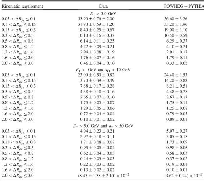
TABLE VI. Measured differential cross section dσ=d_ΔR_μγ in pb. For the data values, the first uncertainty is statistical and the second is systematic. For the theory values, the uncertainty combines statistical, PDF, and renormalization/factorization scale components.

Kinematic requirement Data POWHEGþPYTHIA

E_T>5_.0_GeV

0_.05_<ΔRμγ≤0_.1 53_.900_.762_.00 56_.603_.26 0_.1_<ΔRμγ ≤0_.15 31_.900_.591_.20 33_.201_.96 0_.15_<ΔRμγ≤0_.3 18_.400_.250_.67 19_.001_.10 0_.3<_ΔR_μγ ≤0_.5 10_.100_.160_.37 10_.500_.59 0_.5_<ΔRμγ ≤0_.8 6_.140_.110_.25 6_.290_.37 0_.8_<ΔRμγ ≤1_.2 4_.220_.090_.21 4_.100_.24 1_.2_<ΔRμγ ≤1_.6 2_.940_.080_.19 2_.910_.17 1_.6<_ΔR_μγ ≤2_.0 1_.760_.070_.16 1_.790_.11 2_.0_<ΔRμγ ≤3_.0 0_.460_.040_.10 0_.330_.02

E_T> GeV andq_T<10GeV

0_.05_<ΔRμγ≤0_.1 23_.000_.500_.82 24_.401_.53 0_.1<_ΔR_μγ ≤0_.15 13_.700_.390_.49 14_.200_.88 0.15<_ΔRμγ≤0.3 7.880.170.28 8.210.51

0_.3_<ΔRμγ ≤0_.5 4_.380_.100_.16 4_.480_.28 0_.5_<ΔRμγ ≤0_.8 2_.650_.070_.10 2_.670_.17 0_.8<_ΔR_μγ ≤1_.2 1_.750_.050_.07 1_.750_.11 1.2<_ΔRμγ ≤1.6 1.290.050.06 1.250.08

1_.6_<ΔRμγ ≤2_.0 0_.720_.040_.04 0_.790_.05 2_.0_<ΔRμγ ≤3_.0 0_.100_.010_.02 0_.090_.01

ET>5.0GeV andqT>50GeV

0_.05<_ΔRμγ≤0.1 4.940.230.21 5.070.27

0_.1_<ΔRμγ ≤0_.15 2_.970_.180_.11 3_.050_.18 0_.15_<ΔRμγ≤0_.3 1_.710_.080_.07 1_.730_.09 0_.3_<ΔRμγ ≤0_.5 0_.950_.050_.04 0_.980_.06 0_.5<_ΔRμγ ≤0.8 0.620.040.03 0.580.03

rises from 60% for ET between 5 and 10 GeV to

approximately 90% for ET>50GeV and is nearly the

same in the data and simulation. We take the difference added in quadrature to the statistical uncertainties of the efficiencies as the systematic uncertainty.

As described briefly in Sec.V, the unfolding procedure has been cross-checked in several ways. To assess a systematic uncertainty due to unfolding, we use the small discrepancies observed in the closure test.

The uncertainty in the background estimate is dominated by the uncertainties associated with the corrections that we obtained from the control region (Sec.IV). The statistical uncertainty in the weights for jet multiplicity has a negligible impact, as does the correction for charged hadrons in the photon isolation cone. The parametrized functions to correct the photon distributions in ET andη

carry statistical uncertainties that we propagate to the measured cross sections through simplified MC models. Since the nonprompt photonET,η, andΔRμγ distributions

in the control and signal regions are indistinguishable, we do not assess any uncertainty in the modeling.

The uncertainties in the non-DY backgrounds (t¯_{t and} diboson production) are obtained from the uncertainties in the theoretical cross sections, the luminosity, and the statistical uncertainty in the simulated event samples. We assign 50% uncertainty to the Wþjets and multijet back-ground estimates, which are quite small.

The systematic uncertainty from the simulation of pileup depends primarily on the assumed cross section for

additional pp collisions (roughly the same as the mini-mum-bias cross section) [25]. We vary the value of this cross section by 5% and evaluate the impact on the unfolded spectra.

The uncertainty in the integrated luminosity is 2.2%[26]. Theoretical uncertainties have been calculated and per-tain to the reported theoretical prediction only. We propa-gated the uncertainty due to parton distribution functions (PDFs) using the prescription of Ref. [27]. We vary the factorization/renormalization scale parameters by a factor of 2 to estimate associated scale uncertainties introduced due to neglected higher-order quantum corrections. Finally, we include the MC statistical uncertainty.

VII. RESULTS

The differential cross sections are obtained by sub-tracting the estimated backgrounds from the observed distributions, unfolding the result, and dividing by the bin width and the integrated luminosity,L_¼4_.7_fb−1. No acceptance correction is applied, so these cross sections are defined relative to the kinematic and fiducial requirements listed in TableI.

The measured differential cross sections dσ=dET and

dσ=dΔRμγ are displayed in Fig.3 and listed in Tables V

andVI. A bin-centering correction is applied following the method of Ref.[28]; the abscissa of each point is based on the integral of the simulation across the bin and on the bin width. The shaded region represents the prediction and uncertainty from POWHEG_þPYTHIA, obtained at the

T GEN E ) [pb/GeV] γ (_T /dE σ d -4 10 -3 10 -2 10 -1 10 1 10 Data

POWHEG + Pythia6

< 0.5 μ γ R ∆ 0.05 <

γ

-μ

μ

→

Z

CMS

[GeV]

E

10 20 30 40 50 60 70 80 90 100

Data/Theory 0.5 1 1.5 [GeV] T E

10 20 30 40 50 60 70 80 90 100

Std. Dev. _-4-2 0 2 4 T GEN E ) [pb/GeV] γ (_T /dE σ d -4 10 -3 10 -2 10 -1 10 1 10 _Data

POWHEG + Pythia6

< 3.0 μ γ R ∆ 0.5 <

γ

-μ

μ

→

Z

CMS

[GeV]

E

10 20 30 40 50 60 70 80 90 100

Data/Theory 0.5 1 1.5 [GeV] T E

10 20 30 40 50 60 70 80 90 100

Std. Dev. _-4-2 0 2 4

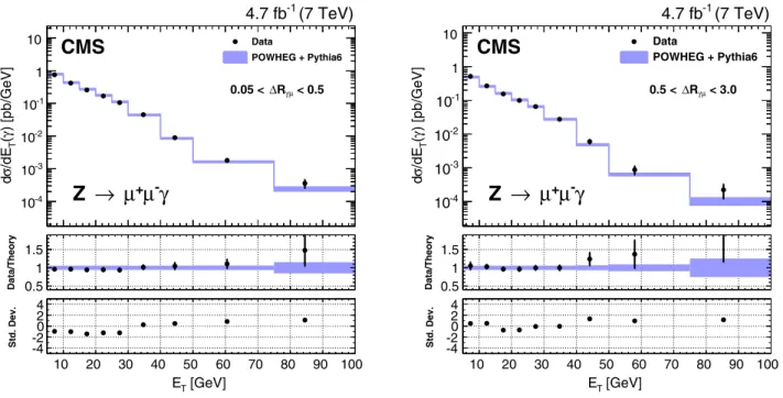
parton level: only the requirements in Table I have been applied to the generator-level muons and photons. The agreement with the data is good.

Energy spectra for photons closer to (0.05_<ΔRμγ ≤

0_.5_{) and farther from the muon (}0_.5_<ΔR

μγ≤3) are

shown in Fig. 4. The rates for photons with large ΔRμγ

and E_T are also well reproduced. The number of events

with30_{< Mμμ <}87_{GeV is about 18% of the number with}

60_{< Mμμ <}120GeV. Of the events with 30_<

Mμμ<87GeV, the fraction of events with at least one

photon with ET>5GeV and 0.05<ΔRμγ ≤0.5 is

8_.70_.1_ðstatÞ 0_.2_ðsystÞ%_{, and with}0_.5_<ΔRμγ ≤3 _is

5.60.1_ðstat_Þ 0.2_ðsyst_Þ%. Photons with _{ΔRμγ >}1.2 and ET>40GeV constitute a small fraction

ð1_.30_.5_ðstatÞ 0_.6_ðsystÞÞ×10−4.

T GEN E ) [pb/GeV] γ ( T /dE σ d -5 10 -4 10 -3 10 -2 10 -1 10 1 10 Data

POWHEG + Pythia6

< 10 [GeV]

T q

γ

-μ

μ

→

Z

CMS

[GeV]

E

10 20 30 40 50 60 70 80 90 100

Data/Theory 0.5 1 1.5 [GeV] T E

10 20 30 40 50 60 70 80 90 100

Std. Dev. _-4-2 0 2 4 γ μ R ∆ GEN

) [pb] _μ

γ R ∆ /d( σ d -1 10 1 10 2 10 Data

POWHEG + Pythia6

< 10 [GeV]

T q

γ

-μ

μ

→

Z

CMS

R

∆

0 0.5 1 1.5 2 2.5 3

Data/Theory 0.5 1 1.5 μ γ R ∆

0 0.5 1 1.5 2 2.5 3

Std. Dev. _-4-2 0 2 4 T GEN E ) [pb/GeV] γ (_T /dE σ d -4 10 -3 10 -2 10 -1 10 1 Data

POWHEG + Pythia6

> 50 [GeV]

T q

γ

-μ

μ

→

Z

CMS

[GeV]

E

10 20 30 40 50 60 70 80 90 100

Data/Theory 0.5 1 1.5 [GeV] T E

10 20 30 40 50 60 70 80 90 100

Std. Dev. _-4-2 0 2 4 γ μ R ∆ GEN ) [pb] μ γ R ∆ /d( σ d -1 10 1 10 2 10 _Data

POWHEG + Pythia6

> 50 [GeV]

T q

γ

-μ

μ

→

Z

CMS

R

∆

0 0.5 1 1.5 2 2.5 3

Data/Theory 0.5 1 1.5 μ γ R ∆

0 0.5 1 1.5 2 2.5 3

Std. Dev. _-4-2 0 2 4

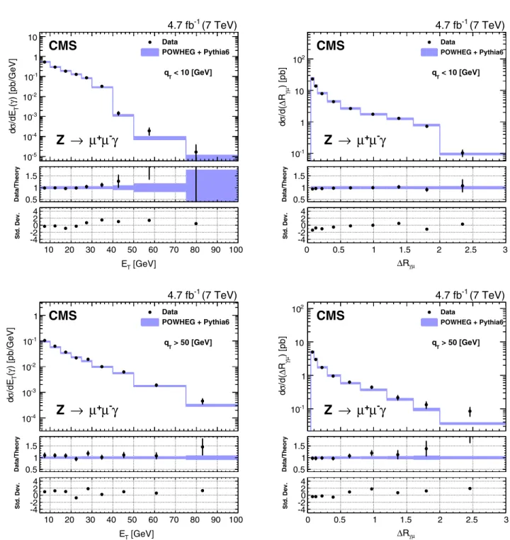
FIG. 5 (color online). Measured differential cross sectionsdσ=dE_T anddσ=d_ΔR_μγ forq_T<10_{GeV (top row) and}q_T>50_GeV

(bottom row). The dots with error bars represent the data, and the shaded bands represent the POWHEGþPYTHIA calculation

We define two subsamples of signal events, one with the Z boson transverse momentumq_T<10GeV, and the other with q_T>50 _{GeV. The measured cross sections} shown in Fig. 5 demonstrate rather different energy spectra for these two cases, thoughdσ=dΔRμγis basically

the same.

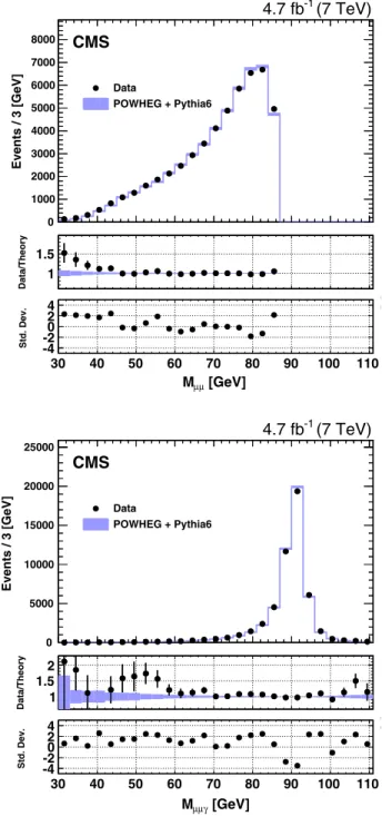
As a final illustration of the nature of this event sample, we present distributions of dimuon mass (Mμμ)

and the three-body mass (Mμμγ) in Fig. 6. The small

increase in the ratio of data to theory forMμμ <40GeV

reflects the insufficient next-to-leading-order accuracy of the simulation; the kinematic requirements on the muons induce a loss of acceptance that require higher-order QCD corrections, as discussed in Ref. [17]. Although the masses of the dimuon pairs populate the tail of the Z resonance (in fact they were selected this way), the three-body mass distribution displays a nearly symmet-ric resonance peak at the mass of the Z boson, thereby confirming the identity of these events as radiative decays Z→μþμ−γ.

VIII. SUMMARY

A study of final-state radiation in Z boson decays was presented. This study serves to test the simulation of events where mixed QED and QCD corrections are important. The analysis was performed on a sample of pp collision data at ffiffiffi

s p

¼7_{TeV recorded in 2011} with the CMS detector and corresponding to an inte-grated luminosity of 4_.7_fb−1. Events with two oppo-sitely charged muons and an energetic, isolated photon were selected with only modest backgrounds. The differential cross sections dσ=dET and dσ=dΔRμγ were

measured for photons within the fiducial and kinematic requirements specified in Table I, and comparisons of dσ=dE_T for photons close to a muon and far from both muons were made. In addition, the differential cross sections dσ=dE_T and dσ=dΔRμγ were compared for

events with large and small transverse momentum of the Z boson, as computed from the two muons and the photon. Simulations based on POWHEGþPYTHIA reproduce the CMS data well, with discrepancies below 5% for5_{< ET<}50 _{GeV and}0_.05_<ΔR

μγ ≤2as

quan-tified in Tables Vand VI.

ACKNOWLEDGMENTS

We congratulate our colleagues in the CERN accel-erator departments for the excellent performance of the LHC and thank the technical and administrative staffs at CERN and at other CMS institutes for their contributions to the success of the CMS effort. In addition, we grate-fully acknowledge the computing centers and personnel of the Worldwide LHC Computing Grid for delivering so effectively the computing infrastructure essential to our analyses. Finally, we acknowledge the enduring support for the construction and operation of the LHC and the CMS detector provided by the following funding agen-cies: BMWFW and FWF (Austria); FNRS and FWO (Belgium); CNPq, CAPES, FAPERJ, and FAPESP (Brazil); MES (Bulgaria); CERN; CAS, MoST, and NSFC (China); COLCIENCIAS (Colombia); MSES 0

1000 2000 3000 4000 5000 6000 7000 8000

Data

POWHEG + Pythia6

(7 TeV) -1

4.7 fb

CMS

[GeV]

μ μ

M

30 40 50 60 70 80 90 100 110

Data/Theory

1 1.5

[GeV]

μ μ

M

30 40 50 60 70 80 90 100 110

Std. Dev. _-4-2

0 2 4

0 5000 10000 15000 20000 25000

Data

POWHEG + Pythia6

(7 TeV) -1

4.7 fb

CMS

[GeV]

γ μ μ

M

30 40 50 60 70 80 90 100 110

Data/Theory 1

1.5 2

[GeV]

γ μ μ

M

30 40 50 60 70 80 90 100 110

Std. Dev. _-4-2

0 2 4

Events / 3 [GeV]

Events / 3 [GeV]

FIG. 6 (color online). Distributions of the dimuon massMμμ

(top) and the three-body massM_μμγ(bottom). The dots with error bars represent the data, and the shaded bands represent the

POWHEGþPYTHIA prediction. The central panels display

and CSF (Croatia); RPF (Cyprus); MoER, ERC IUT, and ERDF (Estonia); Academy of Finland, MEC, and HIP (Finland); CEA and CNRS/IN2P3 (France); BMBF, DFG, and HGF (Germany); GSRT (Greece); OTKA and NIH (Hungary); DAE and DST (India); IPM (Iran); SFI (Ireland); INFN (Italy); MSIP and NRF (Republic of Korea); LAS (Lithuania); MOE and UM (Malaysia); CINVESTAV, CONACYT, SEP, and UASLP-FAI (Mexico); MBIE (New Zealand); PAEC (Pakistan); MSHE and NSC (Poland); FCT (Portugal); JINR (Dubna); MON, RosAtom, RAS, and RFBR (Russia); MESTD (Serbia); SEIDI and CPAN (Spain); Swiss Funding Agencies (Switzerland); MST (Taipei); ThEPCenter, IPST, STAR, and NSTDA (Thailand); TUBITAK and TAEK (Turkey); NASU and SFFR (Ukraine); STFC (United Kingdom); DOE and NSF (USA). Individuals have received support from the Marie-Curie program and the European Research

Council and EPLANET (European Union); the Leventis Foundation; the A. P. Sloan Foundation; the Alexander von Humboldt Foundation; the Belgian Federal Science Policy Office; the Fonds pour la Formation à la Recherche dans l’_{Industrie et dans}

l’Agriculture (FRIA-Belgium); the Agentschap voor

Innovatie door Wetenschap en Technologie (IWT-Belgium); the Ministry of Education, Youth and Sports (MEYS) of the Czech Republic; the Council of Science and Industrial Research, India; the HOMING PLUS program of the Foundation for Polish Science cofinanced from the European Union, Regional Development Fund; the Compagnia di San Paolo (Torino); the Consorzio per la Fisica (Trieste); MIUR Project No. 20108T4XTM (Italy); the Thalis and Aristeia programs cofinanced by EU-ESF and the Greek NSRF; the National Priorities Research Program by Qatar National Research Fund.

[1] C. Albajar et al. (UA1), Studies of intermediate vector

boson production and decay in UA1 at the CERN proton-antiproton collider,Z. Phys. C44, 15 (1989).

[2] P. Bagnaia et al. (UA2), Evidence for Z0

→eþe− at the

CERN_pp¯ _{collider,Phys. Lett. 129B, 130 (1983).} [3] Y. Li and F. Petriello, Combining QCD and electroweak

corrections to dilepton production in the framework of the

FEWZ simulation code,Phys. Rev. D86, 094034 (2012).

[4] S. Dittmaier, A. Huss, and C. Schwinn,OðαsαÞcorrections

to Drell-Yan processes in the resonance region,Proc. Sci.,

LL2014 (2014) 045 [arXiv:1405.6897].

[5] C. Bernaciak and D. Wackeroth, Combining NLO QCD and electroweak radiative corrections to W-boson production at

hadron colliders in the POWHEG framework,Phys. Rev. D

85, 093003 (2012).

[6] L. Barze, G. Montagna, P. Nason, O. Nicrosini, and F. Piccinini, Implementation of electroweak corrections in the

POWHEG BOX: Single W production, J. High Energy

Phys. 04 (2012) 037.

[7] CMS Collaboration, The CMS experiment at the CERN LHC,J. Instrum. 3, S08004 (2008).

[8] CMS Collaboration, Performance of CMS muon

reconstruction in pp collision events at ffiffiffi

s

p

¼7_{TeV, J.} Instrum.7, P10002 (2012).

[9] CMS Collaboration, Energy calibration and resolution of

the CMS electromagnetic calorimeter in pp collisions at

ffiffiffi

s

p

¼7_{TeV,J. Instrum.8, P09009 (2013).}

[10] CMS Collaboration, Report No. CMS TDR CERN/LHCC 2000-038, 2000,http://cds.cern.ch/record/706847. [11] CMS Collaboration, Report No. CMS TDR CERN/LHCC

2002-026, 2002,http://cdsweb.cern.ch/record/578006. [12] S. Alioli, P. Nason, C. Oleari, and E. Re, NLO vector-boson

production matched with shower in POWHEG, J. High

Energy Phys. 07 (2008) 060.

[13] T. Sjöstrand, S. Mrenna, and P. Skands, PYTHIA 6.4

physics and manual, J. High Energy Phys. 05 (2006)

026.

[14] H.-L. Lai, M. Guzzi, J. Huston, Z. Li, P. M. Nadolsky, J. Pumplin, and C.-P. Yuan, New parton distributions for collider physics,Phys. Rev. D82, 074024 (2010). [15] R. Field, Min-bias and the underlying event at the LHC,

Acta Phys. Pol. B42, 2631 (2011).

[16] S. Agostinelliet al. (GEANT4), GEANT4—a simulation

toolkit, Nucl. Instrum. Methods Phys. Res., Sect. A 506, 250 (2003).

[17] CMS Collaboration, Measurement of the Drell-Yan cross section in pp collisions at ffiffiffi

s

p

¼7_{TeV, J. High Energy} Phys. 10 (2011) 007.

[18] CMS Collaboration, CMS Physics Analysis Summary

Report No. CMS-PAS-PFT-10-001, 2010, http://cds.cern

.ch/record/1247373.

[19] CMS Collaboration, CMS Physics Analysis Summary

Report No. CMS-PAS-PFT-09-001, 2009, http://cds.cern

.ch/record/1194487.

[20] M. Cacciari, G. P. Salam, and G. Soyez, The anti-kt jet

clustering algorithm,J. High Energy Phys. 04 (2008) 063. [21] A. Bodek, A. van Dyne, J. Y. Han, W. Sakumoto, and A. Strelnikov, Extracting muon momentum scale corrections for hadron collider experiments,Eur. Phys. J. C72, 2194 (2012).

[22] G. D’Agostini, A multidimensional unfolding method based

on Bayes’ _{theorem, Nucl. Instrum. Methods Phys. Res.,}

Sect. A362, 487 (1995).

[23] T. Adye, inProceedings of PHYSTAT 2011 Workshop on