© Author(s) 2008. This work is distributed under the Creative Commons Attribution 3.0 License.
Chemistry
and Physics
Characterization of the size-segregated water-soluble inorganic ions
at eight Canadian rural sites
L. Zhang, R. Vet, A. Wiebe, C. Mihele, B. Sukloff, E. Chan, M. D. Moran, and S. Iqbal
Air Quality Research Division, Science and Technology Branch, Environment Canada, 4905 Dufferin Street, Toronto, Ontario, M3H 5T4, Canada
Received: 15 May 2008 – Published in Atmos. Chem. Phys. Discuss.: 21 July 2008 Revised: 4 November 2008 – Accepted: 4 November 2008 – Published: 9 December 2008
Abstract. Size-segregated water-soluble inorganic ions,
in-cluding particulate sulphate (SO24−), nitrate (NO−3), ammo-nium (NH+4), chloride (Cl−), and base cations (K+, Na+, Mg2+, Ca2+), were measured using a Micro-Orifice Uniform Deposit Impactor (MOUDI) during fourteen short-term field campaigns at eight locations in both polluted and remote re-gions of eastern and central Canada. The size distributions of SO24− and NH+4 were unimodal, peaking at 0.3–0.6µm in diameter, during most of the campaigns, although a bi-modal distribution was found during one campaign and a tri-modal distribution was found during another campaign made at a coastal site. SO24−peaked at slightly larger sizes in the cold seasons (0.5–0.6µm) compared to the hot seasons (0.3– 0.4µm) due to the higher relative humidity in the cold sea-sons. The size distributions of NO−3 were unimodal, peaking at 4.0–7.0µm during the warm-season campaigns, and bi-modal, with one peak at 0.3–0.6µm and another at 4–7µm during the cold-season campaigns. A unimodal size distri-bution, peaking at 4–6µm, was found for Cl−, Na+, Mg2+, and Ca2+during approximately half of the campaigns and a bimodal distribution, with one peak at 2µm and the other at 6µm, was found during the rest of the campaigns. For K+, a
bimodal distribution, with one peak at 0.3µm and the other at 4µm, was observed during most of the campaigns. Sea-sonal contrasts in the size-distribution profiles suggest that emission sources and air mass origins were the major fac-tors controlling the size distributions of the primary aerosols while meteorological conditions were more important for the secondary aerosols.
The dependence of the particle acidity on the particle size from the nucleation mode to the accumulation mode was not consistent from site to site or from season to season. Particles in the accumulation mode were more acidic than those in the
Correspondence to: L. Zhang
(leiming.zhang@ec.gc.ca)
nucleation mode when submicron particles were in the state of strong acidity; however, when submicron particles were neutral or weakly acidic, particles in the nucleation mode could sometimes be more acidic. The inconsistency of the dependence of the particle acidity on the particle size should have been caused by the different emission sources of all the related species and the different meteorological conditions during the different campaigns. The results presented here at least partially explain the controversial phenomenon found in previous studies on this topic.
1 Introduction
species and base cations needs to be estimated with sufficient accuracy (Environment Canada, 2005).
Substantial knowledge has been gained on the size distri-butions of the major water-soluble inorganic ions during the past four decades. Non-sea salt sulphate (SO24−) and am-monium (NH+4)were found to be predominantly in the fine particle mode while sea spray SO24−, Cl−, Na+, Mg2+, and
Ca2+were more abundant in the coarse fraction (Milford and Davidson, 1987; Hillamo et al., 1998; Heintzenberg et al., 2000; Parmar et al., 2001; Lestari et al., 2003; Park and Kim, 2004; Xiu et al., 2004; Tsai et al., 2005). Fine and coarse NO−3 were both important to its total mass, and their rela-tive fractions were determined by the process through which they were formed, i.e., by the reaction of gaseous HNO3
with ammonia (fine) or with alkaline species in large par-ticles (coarse) (Kadawaki, 1977; Wolff, 1984; Wall et al., 1988; Zhuang et al., 1999; Parmar et al., 2001; Lee et al., 2008). Many studies have found K+to be mostly in fine
par-ticles (Park and Kim, 2004; Park et al., 2004; Chen et al., 2005), although at some locations, coarse K+ can be sub-stantial (Kriv´acsy and Moln´ar, 1998). In some cases, a bi-modal or tribi-modal distribution is needed to describe the size distribution of inorganic ions (Milford and Davidson, 1987; Zhuang et al., 1999; Lestari et al., 2003). Apparently, the particle size distributions vary greatly with season, location, and air-mass origin (Birmili et al., 2001; Hazi et al., 2003; Tunved et al., 2003; Park et al., 2004; Trebs et al., 2004; Van Dingenen et al., 2005; Abdalmogith and Harrison, 2006; Fis-seha et al., 2006).
Despite some field studies conducted at various locations in eastern North America measuring the chemical composi-tion of size-resolved particles (e.g., Hazi et al., 2003; Ru-pakheti et al., 2005; Lee et al., 2008), there is still a lack of understanding of the size distribution profiles of many par-ticle species in these regions, especially at remote locations in northern Canada where there are no major nearby emis-sion sources. During 2001–2005, fourteen short-term field campaigns were conducted by Environment Canada to mea-sure the size-segregated water-soluble inorganic ions at eight rural and remote sites, which are thought to represent the re-gional background air in their respective locations. Back tra-jectory analysis has been conducted to identify the effects of air-mass origins on the seasonal and geographical patterns of the measured ion mass concentrations and size-distribution profiles. Discussion on the size-dependent particle acidity, based on the charge-equivalent cation/anion ratios, is also presented here.
Although the primary goal of the present study is to char-acterize the size distributions of the background inorganic ions over eastern Canada for improving our future acid de-position, air-quality and climate modelling, and health stud-ies, the results should be useful for applications elsewhere. This is because the physical and chemical mechanisms of the formation of the inorganic ions and the dependence of their
size distributions on the meteorological conditions are sim-ilar everywhere around the world. Since the current study includes both the cold and the warm seasons, and was con-ducted at sites located in both polluted and remote regions, the seasonal and geographical patterns of the observed size distributions and the size-dependent particle acidity will pro-vide valuable information to other regions where only limited data are available.
2 Experimental design and method
2.1 Emission sources and measurement sites
The ion species measured in the fourteen campaigns included SO24−, NO−3, NH+4, Cl−, K+, Na+, Mg2+, and Ca2+. The majority of SO24−, NO−3, and NH+4 in this region exist as sec-ondary particles, i.e., formed from their gaseous precursors (SO2, NOx, and NH3, respectively) through various
chemi-cal reactions (Vet et al., 2001). Mg2+and Ca2+are mainly
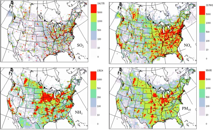
from soil dust emissions, Cl−and Na+from sea salt and road salt emissions, and K+ from soil dust emissions and from biomass burning and vegetation. In order to understand the geographical patterns of the observed ion distributions, emis-sion distributions of the precursors have to be known. Emis-sions of SO2, NOx, NH3, and PM10 (particles with
aerody-namic diameter smaller than 10µm) combining year 2000 Canadian sources and year 2001 USA sources have been ag-gregated into the Canadian air-quality model grids (∼42 km by 42 km) and are shown in Fig. 1. In Canada, southern Ontario and southern Quebec have high emissions of SO2,
NOx, NH3, and PM10since these areas have a high
popula-tion density, many industries, and intense agricultural activi-ties. The southern Prairies of western Canada also have quite high emissions of SO2, NOx, NH3, and PM10 due to
down-stream oil and gas production and agricultural activities. In the USA, most parts of the eastern half of the USA have high emissions of SO2, NOx, NH3, and PM10; however, the
high-est emissions of SO2and NOxare located in the eastern half
of the US Midwest and the Mid-Atlantic, the highest NH3
emissions are located in the central area of the US Midwest (the Great Plains), and the highest PM10 emissions are
lo-cated in most parts of the US Midwest. Seasonal variations of emissions cannot be shown in Fig. 1 and they are briefly discussed wherever needed in Sect. 3.
SO2 NOx
NH3
PM10
SO2 NOx
NH3
PM10
Fig. 1. Maps of emission sources of SO2, NOx(in the equivalent mass of NO2), NH3and PM10based on 2000 Canadian and 2001 US
emission inventory (the unit is tonnes/grid/year with the grid size of∼42 km by 42 km).
However, long-range transport is known to transport pollu-tants from the polluted regions to the remote locations, as will be discussed in Sect. 3.
2.2 Measurement periods
Table 1 lists the time periods when the field campaigns were conducted. Since different sites are located at differ-ent latitudes and some sites are affected by ocean air masses, the traditionally-defined seasons (based on the month of the year) might not be consistent from site to site. Thus, the average daytime (09:00–17:00 local time) air temperature (see Table 1) was used to define the cold-, warm- and hot-season campaigns. Seven campaigns (FRS1, EGB1, ALG1, LED2, CHA2, SPR2, BRL1) were defined as cold-season campaigns, two campaigns (FRS2, KEJ2) were defined as warm-season campaigns, and five campaigns (KEJ1, ALG2, LED1, CHA2, SPR1) were defined as hot-season campaigns. Note that at the three polluted sites, three campaigns were carried out during the cold season (FRS1, EGB1, BRL1) and one during the warm season (FRS2); at the three less pol-luted sites, three campaigns were carried out during the cold season (ALG1, CHA1, SPR2) and three during the hot sea-son (ALG2, CHA2, SPR1); and at the two clean sites, one campaign was carried out during the cold season (LED2),
one during the warm season (KEJ2), and two during the hot season (LED1, KEJ1).
2.3 Sample and analysis
Air samples were collected using a Micro-Orifice Uniform Deposit Impactor sampler (MOUDI Model 110, MSN Min-neapolis, MN, USA) at a mass flow rate of 30 L/min at 0◦C and 1 atm. The sampler was run with 11 fractionation stages with the following 50% cut-off points for the particle aero-dynamic diameters: 18, 9.9, 6.2, 3.1, 1.8, 1.0, 0.54, 0.32, 0.18, 0.093, and 0.048µm, followed by a backup filter. The MOUDI sampler was located 5 m above ground level under a rain shelter that allowed for free ventilation. Teflon® fil-ters of 47 mm diameter and 0.1 mm thickness (PTFE, Sav-illex Corporation, Minnetonka, Minnesota) were used in all stages. After sampling, the filters were stored in pre-washed 10 mL plastic vials at 5–10◦C.
EGB1: Mar06-13, 2002 BRL1: Feb11-Mar4, 2005
FRS1: Nov15-28, 2001 FRS2: May4-16, 2002 ALG1: Feb8-27, 2003 ALG2: Jun5-26, 2003
CHA1: Jan22-Feb21, 2004 CHA2: Jun4-26, 2004 LED1: Aug11-27, 2003 LED2: Oct17-Nov3, 2003
SPR1: Aug17-Sep18, 2004 SPR2: Nov16-Dec12, 2004 KEJ1: Jun29-Jul15, 2002 KEJ2: Oct25-Nov15, 2002 Bratt’s Lake
Algoma
Egbert Sprucedale
Chalk River
Frelighsburg Kejimkujik Lac Edouard
Fig. 2. Locations of the eight measurement sites and the six trajectory clusters at these sites defined from the average of 2001–2005 three-day six-hour back trajectories. Number in the bracket positioned at the end of each cluster represents the percentage of all trajectories associated with that cluster during the specific campaign period.
negative and “no response” values from the laboratory with 2/3 of their reported analytical detection limit (BDL). The BDL was described as 3 standard deviations of repeated mea-surements of a quality control solution at about 40 parts per trillion (ppt). Air concentrations for each aerosol species were then calculated as:Ci=(Mi−BVi)/(MF R∗Et ), where
Ci,Mi andBVi are concentration, collected mass and blank
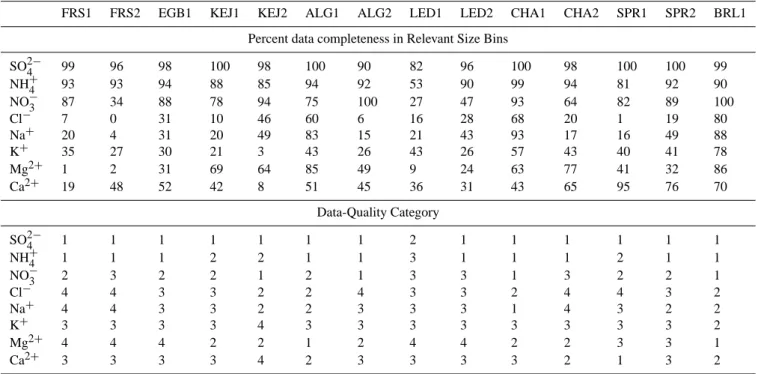
value, respectively, of species i during one sample period (Et )and MFR is the mass flow rate (so MFR∗Etrepresents sampled air volume). The sampling duration (Et )ranged from 6 to 152 h (Table 1) depending on the perceived concen-tration levels at the time of sampling. The number of samples during each campaign is listed in Table 1.
2.4 Quality of MOUDI data
All samples were plotted for data quality control purposes. It was not uncommon that concentrations were lower than the 3-times standard deviation of all blanks divided by the mean air volume sampled (3SDB). Under such circumstances, the data were not quantitative due to a large noise-to-signal prob-lem. For each ion species and for every campaign, the per-centage of samples having a concentration lower than blank values (3SDB) was calculated. When calculating these per-centages, only samples from stages 3–10 (mid-point size 6.2 to 0.093µm) were used for SO24−, NO−3, NH3, and K+
Table 1. List of 14 field campaigns.
Campaign Site Lat N, long W Campaign period Mean daytime Hourly Number Sample temperature average of duration (◦C) RH (%) Samples (h)
FRS1 Frelighsberg, Quebec 45.05, 73.06 15–28 Nov 2001 7 17 6–25
FRS2 4–16 May 2002 12 64 7 11–48
EGB1 Egbert, Ontario 44.23, 79.78 6–13 Mar 2002 2 86 8 6–16
KEJ1 Kejimkujik, Nova Scotia 44.43, 65.21 29 Jun–15 Jul 2002 23 76 17 8–47
KEJ2 25 Oct–15 Nov 2002 6 86 20 13–25
ALG1 Algoma, Ontario 47.04, 84.38 8–27 Feb 2003 −13 72 13 19–71
ALG2 5–26 Jun 2003 22 59 24 10–50
LED1 Lac Edouard, Quebec 47.68, 72.44 11–27 Aug 2003 19 83 12 24–48
LED2 17 Oct–3 Nov 2003 2 87 9 21–72
CHA1 Chalk River, Ontario 46.06, 77.40 22 Jan–21 Feb 2004 −10 65 14 8–127
CHA2 4–26 Jun 2004 19 68 11 24–119
SPR1 Sprucedale, Ontario 45.42, 79.49 17 Aug–18 Sep 2004 19 79 17 24–96
SPR2 16 Nov–12 Dec 2004 0 90 12 13–152
BRL1 Bratt’s Lake, Saskatchewan 50.20, 104.20 11 Feb–4 Mar 2005 −8 93 11 21–106
samples from stages 1–8 (sizes larger than 0.32µm) were used for the other four species. The data were grouped into four data-quality categories based on these percentage num-bers and based on scrutiny of the size-distribution plots. This is because, under certain circumstances, a clear peak in the size distribution was evident from all samples, yet the per-centage of samples having concentrations higher than blank values (3SDB) was very low due to the extremely low con-centrations in the stages not corresponding to the peak sizes. Under this scenario, the data were believed to represent the real size distribution profiles. The percentage numbers (using samples from MOUDI stages 3–10 for SO24−, NO−3, NH3,
and K+ and stages 1–8 for the other four species) and the defined data quality category are all shown in Table 2.
For SO24−, NO−3, and NH+4, 90–100%, 80–90%, and <80% of data from categories 1, 2, and 3, respectively, had concentrations higher than their respective blank values (3SDB). No category 4 data were identified for these three ion species. For the other five species, 85–100% and 50–85% of categories 1 and 2 data, respectively, had concentrations higher than their respective blank values (3SDB) values; the rest of the data were identified as categories 3 and 4, based mainly on the plotted size-distribution profiles. Data belong-ing to categories 1 and 2 were thought to be reliable while data belonging to categories 3 and 4 were less reliable. Note that errors caused by chemical transformation (e.g., NH4NO3
volatility) during the sampling process were not considered in this approach. As a short summary, data for SO24− and NH+4 during all fourteen campaigns and data for NO−3 dur-ing most of the campaigns were of good quality in categories 1 and 2. For the rest of the species, the data quality ranged from relatively good (category 2) to very poor (category 4) depending on the nature of the site and the time of the year.
2.5 Back trajectory cluster analysis
In order to identify the source regions of the sampled aerosols and to better explain the geographical and seasonal patterns of the observed concentrations and size distributions, back trajectory cluster analyses, similar to the approach used in many previous studies (Abdalmogith and Harrison, 2005, and references therein), were conducted. Cluster analysis can account for variations in transport speed and direction simultaneously, yielding clusters of trajectories having simi-lar length and curvature. Three-day back trajectories (every six hours) created by the Canadian Meteorological Centre for the period of 2001–2005 were run through a K-means clus-tering technique for each site. They were organized into six common clusters based on the commonality of Euclidian dis-tance from trajectory to trajectory (Dorling, 1992). Figure 2 shows the six clusters at the eight sites where the fourteen campaigns were conducted.
Table 2. Percentage of data from selected size stages (3–10 stages for SO24−, NH+4, NO3−and K+and 1–8 stages for Cl−, Na+, Mg2+ and Ca2+)having concentrations higher than their respective 3SDB (3 times standard deviation of all blanks divided by the mean sample volume) and defined data-quality categories for all particle species during 14 campaigns (1 represents most reliable and 4 represents least reliable).
FRS1 FRS2 EGB1 KEJ1 KEJ2 ALG1 ALG2 LED1 LED2 CHA1 CHA2 SPR1 SPR2 BRL1
Percent data completeness in Relevant Size Bins
SO24− 99 96 98 100 98 100 90 82 96 100 98 100 100 99
NH+4 93 93 94 88 85 94 92 53 90 99 94 81 92 90
NO−3 87 34 88 78 94 75 100 27 47 93 64 82 89 100
Cl− 7 0 31 10 46 60 6 16 28 68 20 1 19 80
Na+ 20 4 31 20 49 83 15 21 43 93 17 16 49 88
K+ 35 27 30 21 3 43 26 43 26 57 43 40 41 78
Mg2+ 1 2 31 69 64 85 49 9 24 63 77 41 32 86
Ca2+ 19 48 52 42 8 51 45 36 31 43 65 95 76 70
Data-Quality Category
SO24− 1 1 1 1 1 1 1 2 1 1 1 1 1 1
NH+4 1 1 1 2 2 1 1 3 1 1 1 2 1 1
NO−3 2 3 2 2 1 2 1 3 3 1 3 2 2 1
Cl− 4 4 3 3 2 2 4 3 3 2 4 4 3 2
Na+ 4 4 3 3 2 2 3 3 3 1 4 3 2 2
K+ 3 3 3 3 4 3 3 3 3 3 3 3 3 2
Mg2+ 4 4 4 2 2 1 2 4 4 2 2 3 3 1
Ca2+ 3 3 3 3 4 2 3 3 3 3 2 1 3 2
ion species for each trajectory cluster were generated from the 2001–2005 CAPMoN data (Table 3).
It can be seen from Table 3 that the highest concentra-tions of SO24−, NO−3, and NH+4 were associated with clusters SSW at Algoma, SSE and WNW L at Bratt’s Lake, WSW at Chalk River, SSE and WSW at Egbert, WSW at Frelighs-burg, WNW at Kejimkujik, WSW at Lac Edouard, and WSW Sprucedale. Air masses associated with NNE and NNW had the lowest concentrations of SO24−, NO−3, and NH+4 at Al-goma, Chalk River, Egbert, Kejimkujik, Lac Edouard, and Sprucedale. At many locations (e.g., ALG, BRL, CHA, KEJ, LED and SPR), the clusters associated with the highest con-centrations of SO24−, NO−3, and NH+4 were also associated with the highest concentrations of K+, Mg2+, and Ca2+due to the similar geographical patterns of the emissions of SO2,
NOx, NH3, and PM10at these locations.
The 5-year average concentrations showed clear geograph-ical patterns for most species. For example, EGB, FRS, SPR, and ALG had higher SO24− concentrations compared to the rest of the sites, while EGB, FRS, and BRL had higher con-centrations of NO−3, NH+4, and Ca2+, and KEJ and FRS had higher concentrations of Cl− and Na+. Geographical pat-terns of K+and Mg2+were not apparent due to the very low concentrations of these two species, although BRL showed the highest concentrations.
It is known that the slowest (i.e., shortest) trajectory clus-ters passing over high emission areas will have the highest pollutant concentrations and the fastest clusters from clean areas will have the lowest concentrations (Hazi et al., 2003). Results shown in Table 3 support this theory, when compar-ing the defined trajectory clusters shown in Fig. 2 with the emission distributions shown in Fig. 1. The information pro-vided above will be used to support the discussions presented in Sect. 3.
3 Results
Table 3. Mean and median (left and right column separated by ‘,’) atmospheric concentrations (µg m−3)of SO24−, NO−3, NH+4, Cl−, Na+, K+, Mg2+and Ca2+generated from CAPMoN monitored data during the period of 2001–2005.
Site Cluster SO24− NO−3 NH+4 Cl− Na+ K+ Mg2+ Ca2+
ALG ESE 2.29, 1.19 0.33, 0.11 0.70, 0.34 0.01, 0.00 0.04, 0.02 0.04, 0.03 0.03, 0.01 0.12, 0.04 NNE 0.72, 0.58 0.22, 0.10 0.22, 0.14 0.02, 0.01 0.05, 0.03 0.02, 0.02 0.02, 0.01 0.06, 0.03 NNW 0.76, 0.66 0.30, 0.11 0.23, 0.13 0.04, 0.01 0.07, 0.04 0.02, 0.02 0.03, 0.01 0.08, 0.03 SSW 4.04, 2.60 1.32, 0.41 1.54, 1.12 0.02, 0.01 0.05, 0.02 0.07, 0.06 0.05, 0.02 0.25, 0.11 WNW 1.10, 0.91 0.70, 0.17 0.47, 0.27 0.02, 0.00 0.05, 0.02 0.03, 0.02 0.03, 0.02 0.12, 0.06 WNW:L 1.69, 1.20 0.61, 0.16 0.61, 0.34 0.02, 0.01 0.04, 0.02 0.04, 0.03 0.03, 0.02 0.15, 0.06
BRL NNE 1.23, 1.05 0.83, 0.56 0.56, 0.47 0.04, 0.01 0.05, 0.03 0.07, 0.05 0.12, 0.07 0.44, 0.23 NNW 0.85, 0.74 0.74, 0.49 0.40, 0.29 0.06, 0.02 0.06, 0.04 0.10, 0.05 0.11, 0.06 0.40, 0.21 SSE 1.55, 1.29 1.22, 0.70 0.71, 0.50 0.03, 0.02 0.08, 0.03 0.12, 0.07 0.17, 0.10 0.67, 0.40 WNW 0.75, 0.56 0.92, 0.54 0.39, 0.26 0.05, 0.03 0.09, 0.03 0.10, 0.06 0.12, 0.06 0.45, 0.25 WNW:L 1.31, 1.11 1.27, 0.77 0.68, 0.50 0.04, 0.02 0.07, 0.04 0.10, 0.07 0.14, 0.07 0.51, 0.26 WSW 0.92, 0.63 1.30, 0.68 0.55, 0.29 0.05, 0.03 0.10, 0.04 0.09, 0.06 0.10, 0.06 0.41, 0.24
CHA ESE 2.30, 1.48 0.41, 0.13 0.72, 0.43 0.02, 0.01 0.07, 0.03 0.06, 0.05 0.02, 0.02 0.12, 0.05 NNE 0.85, 0.63 0.25, 0.10 0.24, 0.13 0.04, 0.01 0.08, 0.05 0.03, 0.02 0.02, 0.01 0.08, 0.03 NNW 0.87, 0.73 0.36, 0.14 0.27, 0.15 0.08, 0.01 0.11, 0.05 0.03, 0.02 0.03, 0.02 0.09, 0.04 WNW 1.50, 1.13 0.68, 0.19 0.59, 0.33 0.05, 0.01 0.08, 0.03 0.04, 0.04 0.03, 0.02 0.11, 0.06 WNW:L 2.14, 1.34 0.46, 0.16 0.69, 0.38 0.03, 0.01 0.07, 0.03 0.05, 0.04 0.03, 0.02 0.13, 0.06 WSW 3.70, 2.46 0.92, 0.26 1.32, 1.02 0.03, 0.01 0.06, 0.03 0.08, 0.06 0.03, 0.02 0.15, 0.07
EGB NNE 1.57, 1.15 1.53, 0.74 0.75, 0.47 0.14, 0.05 0.12, 0.05 0.05, 0.04 0.08, 0.06 0.99, 0.46 NNW 1.37, 1.11 1.84, 0.90 0.77, 0.47 0.32, 0.08 0.24, 0.07 0.04, 0.04 0.09, 0.07 1.04, 0.54 SSE 5.31, 3.42 2.74, 1.86 2.26, 1.67 0.12, 0.04 0.10, 0.05 0.08, 0.07 0.10, 0.06 1.08, 0.52 WNW 1.97, 1.49 2.66, 1.34 1.22, 0.77 0.19, 0.06 0.14, 0.05 0.05, 0.04 0.08, 0.06 0.78, 0.42 WNW:L 3.52, 2.30 3.12, 2.00 1.76, 1.27 0.19, 0.06 0.15, 0.05 0.07, 0.06 0.10, 0.07 1.16, 0.57 WSW 4.91, 3.60 3.45, 2.05 2.37, 1.83 0.12, 0.05 0.10, 0.05 0.09, 0.08 0.10, 0.06 0.87, 0.48
FRE ENE 1.40, 1.05 0.73, 0.39 0.61, 0.46 0.06, 0.02 0.10, 0.04 0.04, 0.04 0.03, 0.02 0.22, 0.13 NNW 1.17, 0.89 0.93, 0.65 0.55, 0.39 0.24, 0.05 0.22, 0.09 0.04, 0.04 0.04, 0.04 0.41, 0.30 NNW:L 1.39, 1.07 0.97, 0.64 0.66, 0.50 0.15, 0.03 0.15, 0.06 0.05, 0.04 0.04, 0.03 0.35, 0.28 SSW 3.51, 2.37 1.11, 0.64 1.45, 1.02 0.09, 0.02 0.12, 0.04 0.06, 0.06 0.03, 0.03 0.27, 0.18 WNW 2.11, 1.51 1.35, 0.81 1.02, 0.76 0.14, 0.03 0.14, 0.04 0.05, 0.05 0.04, 0.03 0.35, 0.25 WSW 4.12, 2.91 1.84, 0.99 1.87, 1.48 0.09, 0.03 0.11, 0.05 0.08, 0.07 0.04, 0.03 0.37, 0.25
KEJ ESE 1.33, 1.00 0.30, 0.12 0.26, 0.15 0.40, 0.08 0.39, 0.19 0.04, 0.03 0.05, 0.03 0.05, 0.02 NNE 0.82, 0.73 0.24, 0.19 0.15, 0.11 0.42, 0.26 0.40, 0.31 0.03, 0.02 0.05, 0.04 0.04, 0.03 NNW 1.16, 0.82 0.36, 0.20 0.25, 0.15 0.44, 0.28 0.45, 0.34 0.04, 0.03 0.06, 0.04 0.05, 0.04 SSW 2.68, 1.60 0.27, 0.12 0.51, 0.31 0.31, 0.04 0.40, 0.22 0.06, 0.04 0.05, 0.03 0.04, 0.03 WNW 2.86, 1.92 0.54, 0.28 0.69, 0.47 0.32, 0.09 0.47, 0.33 0.06, 0.05 0.06, 0.04 0.08, 0.04 WNW:L 1.98, 1.27 0.29, 0.18 0.42, 0.25 0.28, 0.07 0.36, 0.26 0.05, 0.03 0.05, 0.03 0.05, 0.03
LED ESE 1.24, 0.89 0.15, 0.06 0.34, 0.21 0.02, 0.01 0.06, 0.02 0.03, 0.03 0.01, 0.01 0.05, 0.02 NNE 0.58, 0.44 0.16, 0.09 0.15, 0.08 0.04, 0.01 0.07, 0.05 0.03, 0.02 0.01, 0.01 0.05, 0.02 NNW 0.68, 0.50 0.22, 0.10 0.18, 0.09 0.07, 0.01 0.10, 0.05 0.02, 0.02 0.02, 0.01 0.05, 0.03 WNW 1.27, 0.94 0.40, 0.14 0.44, 0.23 0.04, 0.01 0.09, 0.03 0.04, 0.03 0.02, 0.01 0.06, 0.03 WNW:L 1.30, 0.84 0.26, 0.11 0.40, 0.21 0.04, 0.01 0.07, 0.03 0.04, 0.03 0.02, 0.01 0.07, 0.03 WSW 3.11, 1.98 0.46, 0.14 1.01, 0.68 0.02, 0.01 0.06, 0.03 0.06, 0.05 0.02, 0.01 0.09, 0.04
Table 4. Campaign-average species mass concentrations (C, µg m−3), fine fraction (PM2.5) species concentrations (Cf, µg m−3)and
percentage of mass in the PM2.5fine fraction (Pf, %) for SO24−, NO−3, NH+4, Cl−, Na+, K+, Mg2+and Ca2+. Standard deviations are
shown after the±. The mean value of 0 represents a value<0.005.
FRS1 FRS2 EGB1 KEJ1 KEJ2 ALG1 ALG2 LED1 LED2 CHA1 CHA2 SPR1 SPR2 BRL1 C(SO24−) 2.46±2.35 2.05±1.88 3.22±1.87 3.41±4.4 1.09±1.2 3.98±5.23 2.91±4.37 1.46±3.76 0.65±0.79 1.63±1.69 2.44±1.62 4.45±5.84 0.88±0.38 1.16±0.63 Cf(SO24−) 2.34±2.31 2±1.84 3.07±1.74 3.26±4.19 0.86±0.74 3.64±4.42 2.85±4.31 1.41±3.68 0.61±0.76 1.55±1.62 2.32±1.54 4.32±5.66 0.82±0.35 1.04±0.58 Pf(SO24−) 95 98 96 96 79 91 98 97 95 95 95 97 93 90
C(NO−3) 1.77±2.2 0.13±0.18 3.13±2.44 0.55±0.63 0.34±0.65 3.62±3.31 0.29±0.4 0.09±0.17 0.28±0.67 0.87±2.09 0.16±0.09 0.33±0.46 0.33±0.4 2.36±1.9
Cf(NO−3) 1.52±1.99 0.05±0.06 2.8±2.22 0.17±0.18 0.09±0.12 2.83±2.42 0.07±0.08 0.02±0.02 0.23±0.55 0.73±1.83 0.05±0.04 0.11±0.29 0.26±0.36 2.07±1.73
Pf(NO−3) 86 37 90 31 25 78 24 23 83 84 28 33 79 88
C(NH+
4) 1.37±1.35 0.77±0.73 2±1.24 1.05±1.22 0.25±0.38 1.94±2.54 1.08±1.59 0.41±1.06 0.24±0.45 0.67±1.06 0.78±0.54 1.42±1.89 0.31±0.23 1.05±0.63
Cf(NH+4) 1.32±1.32 0.76±0.73 1.96±1.2 1.03±1.19 0.2±0.24 1.8±2.1 1.06±1.57 0.41±1.04 0.23±0.43 0.65±1.04 0.76±0.53 1.39±1.84 0.29±0.22 0.99±0.59
Pf(NH+4) 97 99 98 98 80 92 98 98 95 97 97 98 95 94
C(Cl−) 0.06±0.06 0.01±0.01 0.23±0.11 0.16±0.24 0.42±0.44 0.48±0.39 0.01±0.01 0.05±0.06 0.02±0.03 0.12±0.17 0.01±0.02 0.01±0.01 0.02±0.02 0.07±0.05 Cf(Cl−) 0.04±0.06 0.01±0 0.1±0.06 0.02±0.03 0.04±0.05 0.22±0.2 0.01±0.01 0.02±0.03 0.01±0.02 0.04±0.04 0.01±0.01 0±0 0.01±0.01 0.04±0.03
Pf(Cl−) 71 69 42 14 11 45 58 49 64 34 59 53 49 65
C(Na+) 0.06±0.04 0.02±0.01 0.19±0.07 0.24±0.33 0.34±0.44 0.43±0.29 0.02±0.02 0.05±0.04 0.02±0.02 0.15±0.16 0.02±0.02 0.03±0.02 0.04±0.01 0.04±0.02
Cf(Na+) 0.03±0.02 0.01±0.01 0.07±0.03 0.07±0.09 0.05±0.07 0.22±0.16 0.01±0.01 0.03±0.03 0.01±0.01 0.07±0.06 0.01±0.01 0.02±0.01 0.02±0.01 0.02±0.01
Pf(Na+) 55 67 35 28 16 51 70 64 69 49 53 64 65 55
C(K+) 0.06±0.04 0.03±0.01 0.11±0.05 0.09±0.07 0.01±0.02 0.16±0.15 0.08±0.08 0.06±0.03 0.03±0.03 0.06±0.06 0.06±0.03 0.06±0.03 0.03±0.02 0.07±0.07 Cf(K+) 0.05±0.03 0.03±0.01 0.08±0.03 0.07±0.07 0.01±0.01 0.12±0.13 0.06±0.07 0.03±0.02 0.02±0.02 0.05±0.05 0.03±0.02 0.04±0.03 0.02±0.01 0.06±0.06
Pf(K+) 82 80 78 83 36 77 72 55 68 88 50 66 77 81
C(Mg2+) 0.01±0.01 0±0.01 0.02±0.01 0.05±0.05 0.04±0.05 0.12±0.07 0.07±0.22 0.01±0.01 0±0 0.02±0.03 0.02±0.01 0.02±0.01 0.01±0 0.05±0.04 Cf(Mg2+) 0±0 0±0 0±0 0.01±0.01 0.01±0.01 0.06±0.05 0.02±0.09 0±0 0±0 0.01±0.01 0.01±0 0±0 0±0 0.01±0.01
Pf(Mg2+) 7 12 23 30 19 45 30 33 51 52 31 21 53 18
C(Ca2+) 0.14±0.2 0.14±0.14 0.23±0.14 0.12±0.12 0.02±0.02 0.41±0.26 0.2±0.26 0.05±0.07 0.02±0.04 0.09±0.25 0.1±0.09 0.16±0.12 0.04±0.02 0.21±0.14 Cf(Ca2+) 0.02±0.02 0.03±0.03 0.08±0.06 0.04±0.04 0.01±0.02 0.12±0.12 0.05±0.09 0.02±0.02 0.01±0 0.03±0.07 0.03±0.06 0.03±0.03 0.02±0.01 0.03±0.02
Pf(Ca2+) 13 21 35 34 44 29 26 30 22 37 29 21 41 17
Table 5. Mass median aerodynamic diameter (MMAD) (inµm) and geometric standard deviation (GSD) (separated by “;”) for total, fine (F) and coarse (C) particles for 8 species measured.
FRS1 FRS2 EGB1 KEJ1 KEJ2 ALG1 ALG2 LED1 LED2 CHA1 CHA2 SPR1 SPR2 BRL1
SO24− 0.45; 2.47 0.28; 2.69 0.44; 2.4 0.38; 2.65 0.67; 3.74 0.5; 2.7 0.29; 2.61 0.44; 2.28 0.47; 2.37 0.42; 2.59 0.42; 2.7 0.46; 2.39 0.56; 2.56 0.43; 2.8
F(SO24−) 0.4; 2.1 0.26; 2.42 0.4; 2.13 0.35; 2.37 0.4; 2.38 0.41; 2.17 0.27; 2.44 0.42; 2.12 0.43; 2.1 0.38; 2.24 0.38; 2.37 0.44; 2.2 0.49; 2.21 0.37; 2.26
C(SO24−) 4.4; 1.45 4.45; 1.47 4.16; 1.41 4.14; 1.45 4.63; 1.47 4.39; 1.46 4.25; 1.47 4.03; 1.46 4.01; 1.45 4.28; 1.47 4.25; 1.48 4.04; 1.49 4.11; 1.45 4.38; 1.45 NO−3 0.63; 2.91 2.03; 3.96 0.55; 2.58 3.15; 2.64 3.93; 2.99 0.73; 3.66 3.76; 4.25 3.41; 4.03 0.79; 3.22 0.63; 3.4 2.58; 5.22 2.41; 5.04 0.98; 3.08 0.48; 2.92
F(NO−3) 0.46; 2.06 0.44; 1.96 1.09; 2.66 1.01; 3.3 0.43; 2.29 0.55; 2.28 0.44; 2.45 0.66; 2.24 0.38; 2.13
C(NO−3) 4.37; 1.42 4.57; 1.41 4.38; 1.4 4.58; 1.44 4.85; 1.46 4.94; 1.46 5.43; 1.43 5.03; 1.41 4.61; 1.47 4.54; 1.45 5.29; 1.43 5.11; 1.43 4.44; 1.46 4.55; 1.46 NH+4 0.43; 2.25 0.26; 2.58 0.41; 2.16 0.35; 2.44 0.67; 3.69 0.46; 2.65 0.28; 2.67 0.42; 2.17 0.5; 2.3 0.39; 2.47 0.38; 2.5 0.45; 2.33 0.53; 2.52 0.39; 2.43
F(NH+4) 0.4; 2.04 0.25; 2.42 0.4; 2.05 0.34; 2.34 0.42; 2.42 0.39; 2.17 0.26; 2.48 0.4; 2.05 0.47; 2.09 0.36; 2.26 0.36; 2.3 0.43; 2.21 0.48; 2.26 0.35; 2.14
C(NH+4) 4.21; 1.43 4.62; 1.48 3.63; 1.29 4.04; 1.48 4.6; 1.48 4.51; 1.44 4.45; 1.51 4.12; 1.46 3.88; 1.44 4.29; 1.48 4.6; 1.52 3.76; 1.48 3.93; 1.43 4.18; 1.43 Cl− 4.38; 1.88 5.64; 2.07 1.87; 5.48 1.77; 4.48 2.11; 6.48 0.86; 5.63
F(Cl−) 0.63; 5.06 0.74; 4.37 0.38; 6.12 0.38; 3.59
C(Cl−) 5.3; 1.42 4.89; 1.41 5.13; 1.43 4.59; 1.49 4.15; 1.43 5.13; 1.47 4.84; 1.49
Na+ 3.49; 1.81 1.75; 4.7 1.28; 4.16 1.79; 4.89 1.16; 5.01
F(Na+) 0.67; 3.79 0.69; 3.61 0.61; 4.06 0.51; 3.53
C(Na+) 4.92; 1.43 4.49; 1.43 4.99; 1.44 4.68;1.48 4.02; 1.43 4.87; 1.47 4.59; 1.48
K+ 0.55; 5.62 1.05; 6.22 0.42; 4.12 1.38; 6.03 0.61; 3.17
F(K+) 0.28; 3.2 0.2; 4.6 0.34; 2.87 0.31; 3.77 0.26; 3.55 0.35; 4.19 0.31; 3.01 0.37; 3.91 0.45; 2.35
C(K+) 4.77; 1.5 4.53; 1.44 4.77; 1.52 5.05; 1.46 4.49; 1.45
Mg2+ 3.4; 3.76 3.48; 2.31 4.7; 2.51 2.56; 3.26 2.27; 7.78 3.11; 3.55 2.25; 2.88 2.91; 4.99
F(Mg2+) 0.86; 3.38 1.4; 2.18 1.23; 2.97 1; 2.44 0.92; 3.13 1.07; 2.18
C(Mg2+) 4.95; 1.47 4.61; 1.45 4.98; 1.44 4.93; 1.49 5.45; 1.45 4.81;1.47 4.65; 1.47 5.18; 1.47
Ca2+ 2.79; 5.65 3.43; 4.95 2.63; 4.04 3.17; 4.66 4.98; 2.6
F(Ca2+) 0.36; 5.3 0.48; 4.73 0.7; 3.52 0.53; 4.16 1.21; 2.62
C(Ca2+) 5.27; 1.47 5.3; 1.46 4.96; 1.44 5; 1.48 5.43; 1.46 5.4; 1.46 5.06; 1.46 5.37; 1.46 5.1; 1.46 5.3; 1.46 5.35; 1.44 5.23; 1.45
concentrations (each sample was weighted by its duration) at the six sites that each had two campaigns, (3) the geo-graphical patterns of the campaign-average concentrations, (4) the fine and coarse fractions of the ion mass concentra-tions, and (5) the characterization of size distributions in-cluding the size-distribution profiles and related parameters. Two campaigns made at Algoma are discussed in more de-tail in Sect. 3.6 considering the strong effects of local sources
(road salt) and the unusual seasonal pattern of several ob-served species (e.g., SO24−, NH+4). Size-dependence of par-ticle acidity is explored in Sect. 3.7 based on the charge-equivalent cation/anion ratios at every MOUDI stage.
Fine particles were defined as the particles having an aero-dynamic diameter smaller than 2.5µm (PM2.5); however,
size-distribution profiles using a modified Twomey inversion technique (Winklmyr et al., 1990) and kernel functions from Marple et al. (1991), as was done in previous studies (e.g., Li et al., 1998). Fine fractions of the total mass were then obtained by integrating the profiles from 0–2.5µm. Within air-quality and climate models where size-resolved aerosols are a concern, a sectional or moment approach is commonly used to describe aerosol size distributions. For the sectional approach, the size-distribution profile presented in Figs. 3 and 4 can be used; for the moment approach, a sum of two or three lognormal distributions is commonly used (e.g., Acker-mann et al., 1998). Thus, in the present study, fine and coarse particles are separately fitted into lognormal distributions for potential future applications. The mass median aerodynamic diameter (MMAD) and associated geometric standard devi-ation (GSD) were calculated for the total mass and for the fine and coarse fractions of the total mass (Table 5). The dis-cussions presented in this section are based on results shown in Tables 4 and 5 and in Figs. 3–6. Information presented in Table 1, Figs. 1 and 2, and Sect. 2.5 is needed to explain the observed phenomenon.
3.1 Sulphate
Fine particle SO24− is commonly generated by the oxida-tion of SO2 through a slow gas-phase (homogeneous)
oxi-dation and/or gas/particle phase (heterogeneous) oxioxi-dation. The rate of SO24−production is expected to be higher in the warm and hot seasons when compared to the cold seasons (see some detailed discussions in Hazi et al., 2003, and refer-ences therein). Coarse SO24−is produced by reactions of SO2
or sulfuric acid on the wet surface of sea salt or soil particles (Wall et al., 1988).
At Frelighsburg, the average SO24− concentration during FRS1 was slightly higher than during FRS2 (Table 4). By looking at the back trajectories shown in Fig. 2, it can be seen that 59% of the air masses during FRS1 (clusters SSW and WSW) were from the high SO2emission regions of eastern
USA and the industrial areas of southern Ontario and south-ern Quebec, while only 25% of the air masses during FRS2 were from these same regions. Thus, despite the slightly colder weather during FRS1, the SO24−concentrations were higher because of the more polluted air masses.
At Chalk River, Sprucedale, and Lac Edouard, the hot-season campaigns generally had a higher percentage of pol-luted air masses (e.g., clusters WSW and ESE clusters were the most polluted and clusters NNW and NNE were the least polluted at all three locations). The campaign-average SO24− concentrations were higher during the hot-season campaigns at all three locations due to a combination of the effects of temperature differences and air-mass origins. The campaign-average SO24−concentration was 50% higher in the hot sea-son compared to the cold seasea-son at Chalk River, >100% higher at Lac Edouard and∼400% higher at Sprucedale.
At Kejimkujik, the campaign-average SO24− concentra-tion was three times higher during the hot-season campaign (KEJ1) compared to the warm-season campaign (KEJ2). This was likely due to a combination of the effects of tem-perature differences and different air-mass origins. During KEJ1, 28% of the air masses were from the high emis-sion region (cluster WNW) and 13% were from the At-lantic Ocean (clusters SSW and ESE) while during KEJ2, these numbers were about the reverse, i.e., 14% and 25%, respectively. Because of the differences in the air-mass origins during these two campaigns, the concentrations of coarse SO24− during KEJ1 were slightly lower than during KEJ2 (0.15 vs. 0.23µg m−3)while concentrations of fine
SO24−during KEJ1 were much higher than during KEJ2 (3.3 vs. 0.9µg m−3).
At Algoma, the campaign-average SO24− concentration was higher during ALG1 than during ALG2. The air-mass origins shown in Fig. 2 cannot explain this phenomenon since ALG1 had a lower percentage of air masses from clus-ters SSW and ESE (passing over high emission regions) and a higher percentage of air masses from NNW and NNE (pass-ing over clean regions) when compared to ALG2. The phe-nomenon is also in contradiction to the theory that SO24− pro-duction was higher during the hot seasons since ALG1 was a cold-season campaign and ALG2 was a hot-season cam-paign. The causes of higher campaign-average concentra-tions during the cold-season campaign at this location will be discussed in Sect. 3.6.
In comparing campaign-average concentrations conducted during the same season, higher SO24− concentrations were observed at locations close to high SO2emission areas and/or
with air masses from high emission sources. For example, SO24−concentrations were higher at locations close to the in-dustrial areas of southern Ontario and southern Quebec (e.g., Sprucedale, Egbert and Frelighsberg) compared to remote lo-cations (e.g., Lac Edouard). The average SO24− concentra-tions varied by>5 times from site to site during any season. The fine fraction of SO24− mass concentrations made up
≥95% of the total SO24− mass in ten campaigns (FRS1, FRS2, EGB1, KEJ1, ALG2, LED1, LED2, CHA1, CHA2, SPR1), around 90% in three campaigns (ALG1, SPR2, BRL1), and 79% in one campaign at a coastal site (KEJ2) in late fall. Note that another campaign at the same coastal site (KEJ1) showed different concentrations (>3 times higher) and fine/total fractions (96%) from those of KEJ2. The dif-ferences were caused by different air-mass origins as shown in Fig. 2. Since fine SO24− particles dominated the total SO24− mass concentrations, their geographical distributions and seasonal variations were similar to the total SO24−mass concentrations (Table 4). Coarse SO24− particle concentra-tions (total minus fine particles) were generally very low, ranging from 0.03–0.32µg m−3 during the fourteen
SPR3 0 0.2 0.4 0.6 0.8 1 1.2
0.01 0.1 1 10
Aerodynamic Diameter dM /d lo g D (µ g m -3) FRS1 0 0.5 1 1.5 2 2.5 3 3.5 4
0.01 0.1 1 10
FRS2 0 0.5 1 1.5 2 2.5 3 3.5
0.01 0.1 1 10
EGB1 0 1 2 3 4 5
0.01 0.1 1 10
KEJ1 0 1 2 3 4 5 6 7 8
0.01 0.1 1 10
KEJ2 0 0.2 0.4 0.6 0.8 1 1.2
0.01 0.1 1 10
ALG1 0 1 2 3 4 5
0.01 0.1 1 10
ALG2 0 1 2 3 4 5
0.01 0.1 1 10
LED1 0 0.5 1 1.5 2 2.5
0.01 0.1 1 10
LED2 0 0.2 0.4 0.6 0.8 1
0.01 0.1 1 10
CHA1 0 0.5 1 1.5 2
0.01 0.1 1 10
CHA2 0 0.5 1 1.5 2 2.5 3
0.01 0.1 1 10
SPR1 0 1 2 3 4 5 6
0.01 0.1 1 10
BRL1 0 0.5 1 1.5 2 2.5 3 3.5
0.01 0.1 1 10
SPR2SPR3 0 0.2 0.4 0.6 0.8 1 1.2
0.01 0.1 1 10
Aerodynamic Diameter dM /d lo g D (µ g m -3) FRS1 0 0.5 1 1.5 2 2.5 3 3.5 4
0.01 0.1 1 10
FRS2 0 0.5 1 1.5 2 2.5 3 3.5
0.01 0.1 1 10
EGB1 0 1 2 3 4 5
0.01 0.1 1 10
KEJ1 0 1 2 3 4 5 6 7 8
0.01 0.1 1 10
KEJ2 0 0.2 0.4 0.6 0.8 1 1.2
0.01 0.1 1 10
ALG1 0 1 2 3 4 5
0.01 0.1 1 10
ALG2 0 1 2 3 4 5
0.01 0.1 1 10
LED1 0 0.5 1 1.5 2 2.5
0.01 0.1 1 10
LED2 0 0.2 0.4 0.6 0.8 1
0.01 0.1 1 10
CHA1 0 0.5 1 1.5 2
0.01 0.1 1 10
CHA2 0 0.5 1 1.5 2 2.5 3
0.01 0.1 1 10
SPR1 0 1 2 3 4 5 6
0.01 0.1 1 10
BRL1 0 0.5 1 1.5 2 2.5 3 3.5
0.01 0.1 1 10
SPR2
Fig. 3. Average size distributions of SO24−, NH+4, and NO−3 during 14 field campaigns.
Because of the very small fractions of coarse SO24− dur-ing most of the campaigns, the SO24− size distribution was dominated by a single mode peaking at 0.3–0.6µm (Fig. 3). A campaign-average trimodal size distribution was apparent at KEJ2 due to the non-negligible coarse SO24− fraction. A very small second peak in the coarse particle size range of 2– 5µm was also observed in several campaigns (e.g., ALG1, SPR2). In general, the SO24−size distribution profiles were similar at different locations and during different seasons;
when the RH seasonal variations were small, the MMAD seasonal variations were also small (e.g., little difference at CHA and very small differences at LED for both RH and MMAD).
The MMAD for SO24−over all campaigns, except KEJ2, ranged from 0.28 to 0.56µm with GSDs around 2.3 to 2.8 (Table 5). The KEJ2 campaign exhibited a higher MMAD and GSD due to the contribution of sea salt sulphate par-ticles. By fitting fine and coarse SO24− particles separately into lognormal distributions, the MMAD ranged from 0.26 to 0.49µm for fine particles and 4.0 to 4.6µm for coarse particles, with the GSD ranging from 2.1 to 2.4 for fine par-ticles and from 1.4 to 1.5 for coarse parpar-ticles. Most previous studies showed the MMAD values ranged from 0.3–0.5µm (Milford and Davidson, 1987). Results shown above confirm that the variations in the MMAD and GSD values of SO24− were caused by different air-mass origins (which control the emissions of the gaseous precursor) and by meteorological conditions (which control physical and chemical processes that produce SO24−and remove it from the atmosphere). 3.2 Nitrate
Fine NO−3 is produced by the gas-phase reaction of HNO3
with NH3while coarse NO−3 is formed by the heterogeneous
reaction of HNO3 gas with sea salt or soil dust particles
(Yoshizumi and Hoshi, 1985). The chemistry favours the production of NH4NO3at high humidity and low
tempera-ture (Allen et al., 1989).
Unlike SO24−, whose concentrations are usually higher in the hot season, NO−3 concentrations are much higher during the cold season due to its favoured low temperature reaction thermodynamics and its volatility in hot weather. This was found to be the case for the campaign-average NO−3 con-centrations at Frelighsberg, Algoma, Chalk River, and Lac Edouard. It is noted that the NO−3 concentrations during FRS1 (November, 2001) were more than ten times higher than during FRS2 (May, 2002) despite the fact that the tem-perature difference during these two campaigns was small (a few degrees). The very large difference in the campaign-average NO−3 concentrations was caused by a combination of the different air-mass origins and different temperatures since a larger percentage of air-mass trajectories were from the high emission regions and the temperature was lower dur-ing FRS1 compared to FRS2. At Sprucedale, no apparent seasonal difference was found, suggesting that the effects of different air-mass origins and the effects of different temper-atures during the two campaigns cancelled each other out. At Kejimkujik, the hot-season campaign had a slightly higher average NO−3 concentration than the warm-season campaign, but the hot season was determined by coarse particle NO−3, consistent with the considerably higher Ca2+concentrations and the more frequent trajectories over the high NOx
emis-sion areas of eastern North America.
Similar to SO24−, higher NO−3 concentrations were found in general at locations close to the high NOxand NH3
emis-sion areas and/or with higher frequencies of air masses over the high emission areas. The campaign-average mass con-centrations of NO−3 ranged from 0.1–3.6µg m−3depending on location and season (Table 4).
The fraction NO−3 mass concentrations in the fine mode were 78–90% during the seven cold-season campaigns (FRS1, EGB1, ALG1, LED2, CHA1, SPR2, and BRL1) and 23–36% during the seven warm-season campaigns (FRS2, KEJ1, KEJ2, ALG2, LED1, CHA2, and SPR1). Thus, as expected from thermodynamics, coarse particle NO−3 dominated in the warm seasons while fine particle NO−3 dominated in the cold seasons (except at Kejimkujik and Sprucedale). This also explains the much higher NO−3 con-centrations during the cold seasons compared to the warm seasons. These results agree with previous studies at differ-ent locations (e.g., Kadowaki, 1976; Fisseha et al., 2006). Note that the fine fraction of the total NO−3 mass concentra-tions also depends on the amount of available NH3as
dis-cussed below in Sect. 3.7. The coarse nitrate fractions in the hot seasons discussed above should be treated as an upper-end estimation due to the possibility of the loss of fine par-ticle NH4NO3collected by MOUDI which could have
exag-gerated the relative importance of coarse versus fine mode nitrates (Lee et al., 2008).
During the seven cold-season campaigns, the campaign-average NO−3 size distributions showed a bimodal distribu-tion with one peak located in the 0.3–0.6µm range and an-other in the 4.0–7.0µm range (Fig. 3). During the seven warm- or hot-season campaigns, NO−3 showed only one coarse mode peak at 4.0–7.0µm. The size distribution pro-files varied significantly with location and season.
The MMAD for fine NO−3 ranged from 0.38 to 0.66µm at non-coastal sites, with GSD ranging from 2.0 to 2.3 (Ta-ble 5). At the coastal site (KEJ1, KEJ2), the MMAD and GSD were around 1.0µm and 3.0, respectively, larger than at other rural sites. The MMAD and GSD for coarse NO−3 were 4.4–5.4µm and 1.4–1.47, respectively. The MMAD and GSD values for both fine and coarse NO−3 are quite close to previous measurements at different locations (e.g., Ruij-grok et al., 1997).
3.3 Ammonium
NH+4 is formed from its gaseous precursor NH3through
gas-phase and aqueous-gas-phase reactions with acidic species (e.g., H2SO4, HNO3, and HCl). Among the reaction products,
(NH4)2SO4 is preferentially formed and the least volatile;
NH4NO3is relatively volatile and NH4Cl is the most volatile.
Volatility increases with increasing air temperature and de-creasing humidity (Pio et al., 1987; Mozurkewich, 1993). Note that NH3 emissions are considerably higher during
increased agricultural activity and temperature-related emis-sions.
It was noted above that SO24−production is higher in the warm/hot seasons. NH+4 production is also expected to be higher in the warm/hot seasons due to higher NH3emissions
and the preference of the formation of (NH4)2SO4. Thus,
the seasonal cycles of NH+4 concentrations should be similar to SO24− at the same locations. This is consistent with the campaign-average SO24−and NH+4 concentrations shown in Table 4.
Higher NH+4 concentrations were found at locations close to high NH3emission areas and/or with a higher frequency of
air masses that traveled over high NH3emission areas. For
example, very high concentrations of NH+4 were observed at Egbert and Bratt’s Lake in the cold season. At Egbert, only 6% of the air masses were from the low NH3
emis-sions clusters (NNW and NNE). At Bratt’s Lake, clusters SSE, WNW L, WNW, NNW all passed over high NH3areas.
Thus, these two campaigns had the highest NH+4 concentra-tions. Both local sources and long-range transport played im-portant roles in the observed high NH+4 concentrations. The campaign-average mass concentrations of NH+4 ranged from 0.2–2.0µg m−3across the region.
The fine fraction of NH+4 mass concentrations constituted 92–99% of the total NH+4 during thirteen of the fourteen campaigns. The only exception was during KEJ2 when the fine fraction was 80% of the total. The dominance of the fine NH+4 fractions shown in Table 4 and in Fig. 3 suggests that most NH+4 was created by homogeneous reactions with a unimodal size distribution peaking at 0.3–0.6µm over most campaigns. A small second mode, with a peak at 6µm, was found during ALG1 and a trimodal distribution was found during KEJ2 at a coastal site. Such trimodal distributions have been observed at other coastal locations and are likely caused by a combination of different physical and chemi-cal processes (e.g., aqueous phase chemistry, condensational growth, droplet evaporation, see discussions in Zhuang et al., 1999). The MMAD and GSD for fine NH+4 were in the range of 0.25–0.48µm and 2.0–2.5, respectively, and for coarse NH+4, in the range of 3.6–4.6µm and 1.3–1.5, respec-tively. Not surprisingly, these values are very close to those of SO24−. These two species also had very similar geograph-ical distributions and size distributions.
3.4 Chloride and sodium
Most Cl− and Na+ measured during the campaigns are
thought to be due to sea salt (KEJ1 and KEJ2) and road salt (other campaigns). Note that salt is spread on the roads in the wintertime in many areas of Canada to melt the ice and snow. The campaign-average concentrations for both Cl−and Na+ were very low during most of the campaigns, but as expected, relatively high during KEJ1 and KEJ2 (coastal site). The KEJ2 campaign had much higher concentrations of Cl−and
Na+ compared to KEJ1 (0.42 vs. 0.16µg m−3for Cl− and
0.34 vs. 0.24µg m−3 for Na+). On the other hand, KEJ2
had much lower concentrations of the rest of the species, e.g., the concentrations of Ca2+and K+ during KEJ2 were only
∼15% of those during KEJ1. The different air-mass origins shown in Fig. 2 certainly played the major role in the con-centration differences of all ion species. By comparing the wind speed observed during these two campaigns and the length of 1-day back trajectories (figure not provided), it was found that the trajectory speeds from the Atlantic Ocean were stronger during KEJ2 than during KEJ1. This also caused higher sea salt emissions during KEJ2. During a cold-season campaign at Algoma, very high concentrations of Cl− and Na+ were observed, which were identified to be caused by a local source of road salt as will be discussed in Sect. 3.6. Note that the concentration ratio of Cl−/Na+ranged from 0.3
to 1.2 during thirteen campaigns (1.75 during BRL1), smaller than the seawater ratio of 1.8. This suggested possible Cl−
depletion during most campaigns; and the extent of Cl− de-pletion should be size-dependent (Yao et al., 2003).
At the coastal site (KEJ1, KEJ2), only around 10% of the Cl− mass and 15–30% of the Na+ mass were found in the fine fraction. At other locations, the fine fraction of Cl−and Na+mass ranged from 35–70%. This is because of limited sea salt penetration from coastal areas.
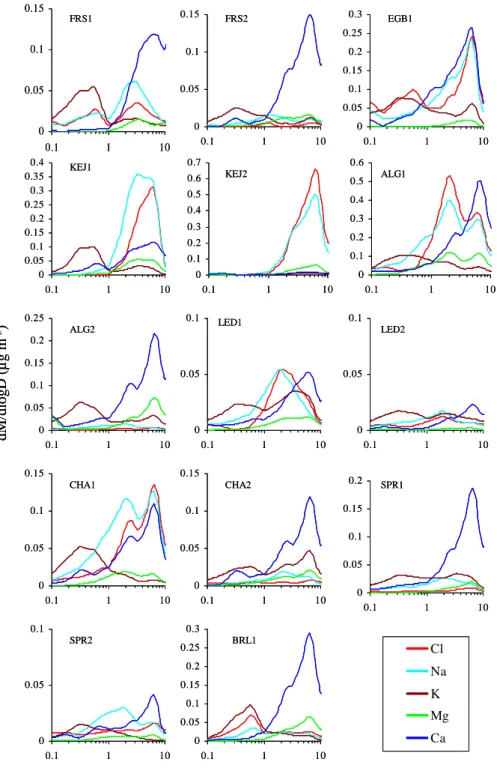
Size distributions of Cl−and Na+ were very similar
dur-ing most of the campaigns, except for KEJ1, which exhibited different modes for Na+and Cl−(Fig. 4). For the campaigns
with very low concentrations, the size distributions shown in Fig. 4 will be highly uncertain due to large measurement un-certainties. For those campaigns with relatively high concen-trations, the size distributions were either unimodal at∼6µm for both Cl−and Na+ during EGB1 and KEJ2 or bimodal, with one mode at 2µm and the other at 6µm, during ALG1 and CHA1. The size distributions of Cl−and Na+were also unimodal during KEJ1, although at a different mode size. Note that during ALG1, the first mode (∼2µm) had higher concentrations than the second mode (∼6µm) while during CHA1, the first mode had lower concentrations compared to the second mode.
The MMAD for Cl−and Na+are only presented in Table 5
for those campaigns in which the concentrations were not too low and the data was of relatively good quality. MMAD for both Cl− and Na+ were around 4–5µm for the coarse fractions and 0.4–0.7µm for the fine fractions. GSD for the coarse and fine fractions were around 1.5 and 3.5–6, respec-tively.
3.5 Potassium, magnesium and calcium
Cl
Na
K
Mg
Ca
FRS1
ALG1 KEJ2
KEJ1
EGB1 FRS2
LED2 LED1
ALG2
BRL1
SPR1
CHA1 CHA2
SPR2 0 0.05 0.1 0.15
0.1 1 10
0 0.05 0.1 0.15
0.1 1 10
0 0.05 0.1 0.15 0.2 0.25 0.3
0.1 1 10
0 0.05 0.1 0.15 0.2 0.25 0.3 0.35 0.4
0.1 1 10
0 0.1 0.2 0.3 0.4 0.5 0.6 0.7
0.1 1 10
0 0.1 0.2 0.3 0.4 0.5 0.6
0.1 1 10
0 0.05 0.1 0.15 0.2 0.25
0.1 1 10
0 0.05 0.1
0.1 1 10
0 0.05 0.1
0.1 1 10
0 0.05 0.1 0.15
0.1 1 10
0 0.05 0.1 0.15
0.1 1 10
0 0.05 0.1
0.1 1 10
0 0.05 0.1 0.15 0.2 0.25 0.3
0.1 1 10
0 0.05 0.1 0.15 0.2
0.1 1 10
dM/
d
lo
g
D
(µ
g
m
-3)
Fig. 4. Average size distributions of Cl−, Na+, K+, Mg2+, and Ca2+during 14 field campaigns.
site. If assuming all Na+was originated from sea salt par-ticles, the sea salt contribution to K+, Mg2+, and Ca2+ can be estimated by comparing the observed mass ratio of K+/Na+, Mg2+/Na+, and Ca2+/Na+ with those of seawa-ter, which has a ratio of 0.037, 0.12, and 0.038, respectively, for K+/Na+, Mg2+/Na+, and Ca2+/Na+. Such an
assump-tion might not work for winter campaigns conducted at loca-tions close to highways (e.g., ALG1, EGB1) considering the chemical composition of the road salt was not necessarily the
0 2 4 6 8 10 12 14 0 5/ 0 6/ 2 003 0 6/ 0 6/ 2 003 0 7/ 0 6/ 2 003 0 8/ 0 6/ 2 003 0 9/ 0 6/ 2 003 1 0/ 0 6/ 2 003 1 1/ 0 6/ 2 003 1 2/ 0 6/ 2 003 1 3/ 0 6/ 2 003 1 4/ 0 6/ 2 003 1 5/ 0 6/ 2 003 1 6/ 0 6/ 2 003 1 7/ 0 6/ 2 003 1 8/ 0 6/ 2 003 1 9/ 0 6/ 2 003 2 0/ 0 6/ 2 003 2 1/ 0 6/ 2 003 2 2/ 0 6/ 2 003 2 3/ 0 6/ 2 003 2 4/ 0 6/ 2 003 2 5/ 0 6/ 2 003 2 6/ 0 6/ 2 003 0 2 4 6 8 10 12 14 16 18 20 22 0 8/ 0 2/ 2 003 0 9/ 0 2/ 2 003 1 0/ 0 2/ 2 003 1 1/ 0 2/ 2 003 1 2/ 0 2/ 2 003 1 3/ 0 2/ 2 003 1 4/ 0 2/ 2 003 1 5/ 0 2/ 2 003 1 6/ 0 2/ 2 003 1 7/ 0 2/ 2 003 1 8/ 0 2/ 2 003 1 9/ 0 2/ 2 003 2 0/ 0 2/ 2 003 2 1/ 0 2/ 2 003 2 2/ 0 2/ 2 003 2 3/ 0 2/ 2 003 2 4/ 0 2/ 2 003 2 5/ 0 2/ 2 003 2 6/ 0 2/ 2 003 2 7/ 0 2/ 2 003 0 0.5 1 1.5 2 2.5 3 3.5 4
ESE NNE NNW SSW WNW WNW:L
Dec, Jan, Feb Mar, Apr, May Jun, Jul, Aug Sep, Oct, Nov
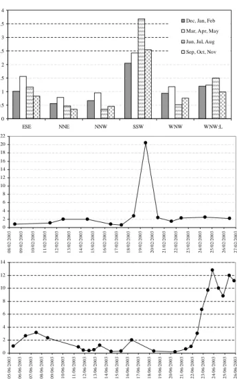
Fig. 5. (a) Median SO24− concentration for 6 trajectory clusters from CAPMoN 2001–2005 daily data, (b) and (c) SO24− concentra-tions from individual samples measured during ALG1 and ALG2, respectively.
At the coastal site, the mass ratios of K+/Na+were found to be 0.03 during one campaign (KEJ2) and 0.37 during an-other campaign (KEJ1). KEJ2 had the lowest K+ concentra-tions among all of the campaigns, but most of the K+during
this campaign was originated from sea salt. On the other hand, only 10% of K+was identified to be from sea salt
dur-ing KEJ1. The difference between these two campaigns was caused by different air-mass origins as discussed in Sect. 3.4. The mass ratios of K+/Na+ were found to be in the range of 1.2–4.0 during the rest of the non-winter campaigns. This suggests that sea salt played no significant role (<3%) as a source of K+at inland sites.
The mass concentrations of Mg2+ were very low (≤0.02µg m−3) during nine campaigns. During the two campaigns made at the coastal site, the mass ratios of Mg2+/Na+were found to be 0.21 (KEJ1) and 0.12 (KEJ2), suggesting that ∼50% of the Mg2+ during KEJ1 and all
of the Mg2+ during KEJ2 were from sea salt. The only
non-winter inland campaign that had Mg2+ concentrations
higher than 0.02µg m−3is ALG2, which had a mass ratio
of Mg2+/Na+equal to 3.5, suggesting little influence of sea salt. Similarly, 7% and 60% of the Ca2+ during KEJ1 and KEJ2, respectively, were from sea salt. For all the rest of the campaigns, sea salt played no significant role in the mass concentration of Ca2+.
Fine particle K+concentrations dominated its total mass concentrations during most of the campaigns. The almost equal amounts of K+in the fine and coarse fractions during KEJ1 and a few other campaigns suggest that emissions from soil dust and emissions from biomass burning and vegeta-tion were equally important. Enhanced K+concentrations in
submicron particles were also found in previous studies (An-dreae, 1983; Gaudichet et al., 1995; Jaffrezo et al., 1998). The size distribution of K+ was bimodal, with one mode peaking at 0.3–0.5µm and the other at 4–6µm.
Coarse particle Mg2+and Ca2+concentrations dominated their respective total mass concentrations during most of the campaigns. Mg2+ and Ca2+ had bimodal distributions (one at 2.5µm and the other at 6µm) during several cam-paigns. In a few campaigns, an extra fine mode was also observed (e.g., Ca2+ in CHA1 and CHA2); however, the concentrations were extremely low and thus, the size distri-butions shown in Fig. 4 might not represent the real situa-tion. The size distribution of Mg2+shown for ALG1 seems
to be real since it also had two modes similar to the other cation species. The multimodal distributions have also been observed at other locations (e.g., Lin et al., 2007). Such a phenomenon could be caused by a mix of different-aged air masses having different modes, e.g., one air mass having new emissions peaking at sizes of 6µm in diameter and another one having an aged air mass peaking at submicron sizes, the latter could be due to the lowest removal rate by dry depo-sition and by precipitation scavenging for this particle size range.
The MMAD for fine and coarse K+ were 0.4–1.4µm and 5µm, respectively. The MMAD for Mg2+were 0.8–
1.4µm for fine fractions and around 5µm for coarse frac-tions, and the corresponding GSD were 2–3 and 5, respec-tively. MMAD and GSD for coarse Ca2+were around 5µm and 1.5, respectively.
3.6 Comparison of campaigns ALG1 and ALG2
0 0.5 1 1.5 0. 0 4 8 0. 09 3 0. 1 8 0. 3 2 0. 5 4 1 1. 8 3. 1 6. 2 9. 9 KEJ2, Oct/Nov 0 0.5 1 1.5 2 0. 0 4 8 0. 09 3 0. 1 8 0. 3 2 0. 5 4 1 1. 8 3. 1 6. 2 9. 9 KEJ1, Jun/Jul 0 0.5 1 1.5 2 2.5 0. 0 4 8 0. 09 3 0. 1 8 0. 3 2 0. 5 4 1 1. 8 3. 1 6. 2 9. 9 SPR2, Nov/Dec 0 0.5 1 1.5 2 2.5 3 3.5 4 0. 0 4 8 0. 09 3 0. 1 8 0. 3 2 0. 5 4 1 1. 8 3. 1 6. 2 9. 9 SPR1, Aug/Sep 0 0.5 1 1.5 2 2.5 3 3.5 4 4.5 5 5.5 0. 0 4 8 0. 0 9 3 0. 1 8 0. 3 2 0. 5 4 1 1. 8 3. 1 6. 2 9. 9 LED2, Oct/Nov 0 0.5 1 1.5 2 2.5 0. 0 4 8 0. 0 93 0. 1 8 0. 3 2 0. 5 4 1 1. 8 3. 1 6. 2 9. 9 CHA1, Jan/Feb 0 0.5 1 1.5 2 2.5 3 3.5 4 4.5 5 5.5 6 6.5 7 0. 0 4 8 0. 0 93 0. 1 8 0. 3 2 0. 5 4 1 1. 8 3. 1 6. 2 9. 9 BRL1, Feb/Mar 0 0.5 1 1.5 2 2.5 3 3.5 4 4.5 5 0. 0 4 8 0. 0 93 0. 1 8 0. 3 2 0. 5 4 1 1. 8 3. 1 6. 2 9. 9 LED1, Aug 0 0.5 1 1.5 2 2.5 3 3.5 4 0. 0 4 8 0. 0 93 0. 1 8 0. 3 2 0. 5 4 1 1. 8 3. 1 6. 2 9. 9 CHA2, Jun 0 0.5 1 1.5 2 2.5 0. 0 4 8 0. 0 9 3 0. 1 8 0. 3 2 0. 5 4 1 1. 8 3. 1 6. 2 9. 9 FRS1, Nov 0 0.5 1 1.5 2 2.5 3 3.5 4 4.5 5 0. 0 4 8 0. 0 9 3 0. 1 8 0. 3 2 0. 5 4 1 1. 8 3. 1 6. 2 9. 9 FRS2, May 0 0.5 1 1.5 2 2.5 0. 0 4 8 0. 0 9 3 0. 1 8 0. 3 2 0. 5 4 1 1. 8 3. 1 6. 2 9. 9 ALG1, Feb 0 0.5 1 1.5 2 2.5 3 3.5 4 4.5 5 5.5 6 0. 0 4 8 0. 0 9 3 0. 1 8 0. 3 2 0. 5 4 1 1. 8 3. 1 6. 2 9. 9 ALG2, Jun 0 0.5 1 1.5 2 0. 0 4 8 0. 0 9 3 0. 1 8 0. 3 2 0. 5 4 1 1. 8 3. 1 6. 2 9. 9 EGB1, Mar 0 0.5 1 1.5 0. 0 4 8 0. 09 3 0. 1 8 0. 3 2 0. 5 4 1 1. 8 3. 1 6. 2 9. 9 KEJ2, Oct/Nov 0 0.5 1 1.5 0. 0 4 8 0. 09 3 0. 1 8 0. 3 2 0. 5 4 1 1. 8 3. 1 6. 2 9. 9 KEJ2, Oct/Nov 0 0.5 1 1.5 2 0. 0 4 8 0. 09 3 0. 1 8 0. 3 2 0. 5 4 1 1. 8 3. 1 6. 2 9. 9 KEJ1, Jun/Jul 0 0.5 1 1.5 2 0. 0 4 8 0. 09 3 0. 1 8 0. 3 2 0. 5 4 1 1. 8 3. 1 6. 2 9. 9 KEJ1, Jun/Jul 0 0.5 1 1.5 2 2.5 0. 0 4 8 0. 09 3 0. 1 8 0. 3 2 0. 5 4 1 1. 8 3. 1 6. 2 9. 9 SPR2, Nov/Dec 0 0.5 1 1.5 2 2.5 0. 0 4 8 0. 09 3 0. 1 8 0. 3 2 0. 5 4 1 1. 8 3. 1 6. 2 9. 9 SPR2, Nov/Dec 0 0.5 1 1.5 2 2.5 3 3.5 4 0. 0 4 8 0. 09 3 0. 1 8 0. 3 2 0. 5 4 1 1. 8 3. 1 6. 2 9. 9 SPR1, Aug/Sep 0 0.5 1 1.5 2 2.5 3 3.5 4 0. 0 4 8 0. 09 3 0. 1 8 0. 3 2 0. 5 4 1 1. 8 3. 1 6. 2 9. 9 SPR1, Aug/Sep 0 0.5 1 1.5 2 2.5 3 3.5 4 4.5 5 5.5 0. 0 4 8 0. 0 9 3 0. 1 8 0. 3 2 0. 5 4 1 1. 8 3. 1 6. 2 9. 9 LED2, Oct/Nov 0 0.5 1 1.5 2 2.5 3 3.5 4 4.5 5 5.5 0. 0 4 8 0. 0 9 3 0. 1 8 0. 3 2 0. 5 4 1 1. 8 3. 1 6. 2 9. 9 LED2, Oct/Nov 0 0.5 1 1.5 2 2.5 0. 0 4 8 0. 0 93 0. 1 8 0. 3 2 0. 5 4 1 1. 8 3. 1 6. 2 9. 9 CHA1, Jan/Feb 0 0.5 1 1.5 2 2.5 0. 0 4 8 0. 0 93 0. 1 8 0. 3 2 0. 5 4 1 1. 8 3. 1 6. 2 9. 9 CHA1, Jan/Feb 0 0.5 1 1.5 2 2.5 3 3.5 4 4.5 5 5.5 6 6.5 7 0. 0 4 8 0. 0 93 0. 1 8 0. 3 2 0. 5 4 1 1. 8 3. 1 6. 2 9. 9 BRL1, Feb/Mar 0 0.5 1 1.5 2 2.5 3 3.5 4 4.5 5 5.5 6 6.5 7 0. 0 4 8 0. 0 93 0. 1 8 0. 3 2 0. 5 4 1 1. 8 3. 1 6. 2 9. 9 BRL1, Feb/Mar 0 0.5 1 1.5 2 2.5 3 3.5 4 4.5 5 0. 0 4 8 0. 0 93 0. 1 8 0. 3 2 0. 5 4 1 1. 8 3. 1 6. 2 9. 9 LED1, Aug 0 0.5 1 1.5 2 2.5 3 3.5 4 4.5 5 0. 0 4 8 0. 0 93 0. 1 8 0. 3 2 0. 5 4 1 1. 8 3. 1 6. 2 9. 9 LED1, Aug 0 0.5 1 1.5 2 2.5 3 3.5 4 0. 0 4 8 0. 0 93 0. 1 8 0. 3 2 0. 5 4 1 1. 8 3. 1 6. 2 9. 9 CHA2, Jun 0 0.5 1 1.5 2 2.5 3 3.5 4 0. 0 4 8 0. 0 93 0. 1 8 0. 3 2 0. 5 4 1 1. 8 3. 1 6. 2 9. 9 CHA2, Jun 0 0.5 1 1.5 2 2.5 0. 0 4 8 0. 0 9 3 0. 1 8 0. 3 2 0. 5 4 1 1. 8 3. 1 6. 2 9. 9 FRS1, Nov 0 0.5 1 1.5 2 2.5 0. 0 4 8 0. 0 9 3 0. 1 8 0. 3 2 0. 5 4 1 1. 8 3. 1 6. 2 9. 9 FRS1, Nov 0 0.5 1 1.5 2 2.5 3 3.5 4 4.5 5 0. 0 4 8 0. 0 9 3 0. 1 8 0. 3 2 0. 5 4 1 1. 8 3. 1 6. 2 9. 9 FRS2, May 0 0.5 1 1.5 2 2.5 3 3.5 4 4.5 5 0. 0 4 8 0. 0 9 3 0. 1 8 0. 3 2 0. 5 4 1 1. 8 3. 1 6. 2 9. 9 FRS2, May 0 0.5 1 1.5 2 2.5 0. 0 4 8 0. 0 9 3 0. 1 8 0. 3 2 0. 5 4 1 1. 8 3. 1 6. 2 9. 9 ALG1, Feb 0 0.5 1 1.5 2 2.5 0. 0 4 8 0. 0 9 3 0. 1 8 0. 3 2 0. 5 4 1 1. 8 3. 1 6. 2 9. 9 ALG1, Feb 0 0.5 1 1.5 2 2.5 3 3.5 4 4.5 5 5.5 6 0. 0 4 8 0. 0 9 3 0. 1 8 0. 3 2 0. 5 4 1 1. 8 3. 1 6. 2 9. 9 ALG2, Jun 0 0.5 1 1.5 2 2.5 3 3.5 4 4.5 5 5.5 6 0. 0 4 8 0. 0 9 3 0. 1 8 0. 3 2 0. 5 4 1 1. 8 3. 1 6. 2 9. 9 ALG2, Jun 0 0.5 1 1.5 2 0. 0 4 8 0. 0 9 3 0. 1 8 0. 3 2 0. 5 4 1 1. 8 3. 1 6. 2 9. 9 EGB1, Mar 0 0.5 1 1.5 2 0. 0 4 8 0. 0 9 3 0. 1 8 0. 3 2 0. 5 4 1 1. 8 3. 1 6. 2 9. 9 EGB1, Mar
Fig. 6. Statistics of cation-anion ratios at every MOUDI stage during the 14 campaigns. The symbol “×” represents median value and the vertical line represents the range of the central 67% data.
of in the summer. Thus, individual samples collected during ALG1 and ALG2 and their associated trajectory clusters and local meteorology were studied in detail.
It was found that the majority of the samples from ALG1 had much higher Cl− and Na+ concentrations than during ALG2, in particular three samples during ALG1. The Trans-Canada Highway, a major transport route, is located 12 km southwest from this site at its closest point. During the win-ter season, road salt (MgCl2in solution and NaCl) and sand
(probably contains Ca2+ and Mg2+) was heavily used to help melt the ice and snow on this highway. Winds coming from any direction between the south and northwest (150– 315◦) would have brought the air to this site that passed over the highway. Thus, the much higher Cl− and Na+ concentrations during ALG1 (>0.4µg m−3) compared to
ALG2 (<0.02µg m−3)were thought to be caused by the lo-cal source of the road salt. The five-year (2001–2005) CAP-MoN daily concentrations also showed that the average con-centrations of Cl− and Na+ in the winter (December, Jan-uary, February) were ∼5 times higher than the rest of the seasons. It also explains why when Cl−and Na+were high, enhanced Ca2+and Mg2+were also sometimes detected.
the five-year (2001–2005) CAPMoN daily data, it was found that the clusters associated with the high emission areas had higher SO24−concentrations in the summer than in the win-ter while the cluswin-ters associated with the clean areas had lower SO24− concentrations in the summer than in the win-ter (Fig. 5a, only median values were shown here, mean val-ues have similar seasonal patterns). For example, clusters SSW, ESE, and WNW L had higher SO24− concentrations in the summer while clusters NNE, NNW, and WNW had lower SO24− concentrations in the summer compared to the winter. The higher SO24−concentrations in the summer from the polluted-clusters were caused by the higher SO24− pro-duction rate. One cause of the lower SO24−concentrations in the summer compared to the winter from the clean-clusters was probably due to the fast removal rate (dry and wet de-position). However, further studies are needed to identify all the possible causes. It is noted that many samples dur-ing ALG1 associated with clean-clusters had a concentration of∼2µg m−3while many samples during ALG2 had a
con-centration of ≤0.5µg m−3 (Fig. 5b and c). This partially
explains the higher SO24−concentrations during ALG1 than during ALG2.
Another reason for the higher SO24−mass concentrations during ALG1 is that there was one 24-h sample (starting at 11:30 on 19 February) that had a very high concentra-tion (∼20µg m−3). The sample was associated with clus-ters SSW and WNW L and the extremely low wind speed on 19 February. As noted in Sect. 2.5, the slow-moving air mass passing over the high emission areas causes high pollutant concentrations, which likely explains the very high concentration of the sample collected on 19 February. It is worth mentioning that the very low mixing heights in the winter will likely have also played a role in the high pol-lutant concentrations associated with the polluted air masses. As a comparison, ALG2 had seven samples during the three-day period (23–25 June) associated with cluster SSW. The concentrations of these seven samples were much higher than the rest of the samples (e.g., 6–12µg m−3versus 0.5– 3µg m−3), but substantially lower than the extreme sample collected on 19 February during ALG1. Thus, despite the higher percentage of air masses associated with polluted tra-jectory clusters during ALG2, the campaign-average concen-trations were 30% lower compared to ALG1. Several other species (NO−3, NH+4, K+, and Ca2+)had day-to-day vari-ations similar to SO24−, as shown in Fig. 5b and c. Thus, these species also had higher campaign-average concentra-tions during ALG1 than during ALG2, although the magni-tudes of the differences between the two campaigns were dif-ferent for the difdif-ferent species due to their difdif-ferent chemical mechanisms and emission sources.
3.7 Size-dependence of particle acidity
Fine particles are known to be responsible for many adverse health effects for which aerosol acidity seems to play a role (see discussions and references in Haze et al., 2003, and Moya et al., 2003). While it is generally believed that sub-micron particles are more acidic than supersub-micron particles, there is no consistent conclusion on the size-dependence of the acidity within the size range of submicron particles (see a detailed discussion and references in Yao et al., 2007). Data collected in the present study can shed some light on how the particle acidity changes with particle size. In this sec-tion, the concentration ratios (in charge equivalents) between the sum of the measured cations (NH+4, K+, Na+, Mg2+, and Ca2+)and the sum of the measured anions (SO2−
4 , NO
−
3, and
Cl−)were calculated separately for every sample and each
MOUDI stage, similar to the approach described in Kermi-nen et al. (2001). The statistics of the cation/anion ratios (median and the central 67% values) are shown in Fig. 6 and are discussed in detail below. Note that the data from the first and the last stage were not included considering their relatively poor data quality (due to the very low ion concen-trations) compared to the other stages.
Supermicron particles were found to be weakly acidic dur-ing two campaigns (FRS1 and KEJ2), close to neutral durdur-ing one campaign (SPR2) and alkaline during the rest of the cam-paigns. Kerminen et al. (2001) suggested that carbonate par-ticles associated with mineral dust probably played a major role in the alkalinity of supermicron particles. The depletion of Cl−might have also played an important role considering
the much smaller Cl−/Na+ratio compared to seawater (see
the discussion in Sect. 3.4). The acidic supermicron parti-cles observed during KEJ2 were certainly caused by the very low concentrations of the dust-originating ion species (Ca2+, Mg2+, K+), as seen in Table 4, due to the large percentage of ocean air masses reaching this location (Fig. 2).
At the three sites having the highest NH3emissions (see
Sect. 2.5), the submicron particles were basically neutral, even during the cold seasons, i.e., the four campaigns (FRS1, FRS2, EGB1, and BRL1) conducted at the three sites. At the rural locations, where NH3emissions were not so high,
the submicron particles were neutral or close to neutral dur-ing the hot seasons (e.g., ALG2, CHA2, LED1, SPR1), but were acidic during the cold seasons (e.g., ALG1, CHA1, LED2, SPR2). This is because more NH3was available in
the warm/hot seasons than in the cold seasons to neutralize the acidic species. At the coastal site, where NH3emissions
were extremely low, the submicron particles were acidic. The acidity was stronger during KEJ2 than during KEJ1 due to the larger percentage of air masses from the ocean. The strong acidity of the submicron particles observed at KEJ is consistent with previously reported high incidences of acidic particles in Atlantic Canada (Brook et al., 1997).