Eects of atmospheric oscillations on the ®eld-aligned
ion motions in the polar
F
-region
S. Oyama1, S. Nozawa2, S. C. Buchert2, M. Ishii1, S. Watari1, E. Sagawa1, W. Kofman3, J. Lilensten3, R. Fujii2
1 Communications Research Laboratory, 4-2-1, Nukuikita-machi, Koganei, Tokyo, 184-8795, Japan
2 Solar-Terrestrial Environment Laboratory, Nagoya University, Furo-cho, Chikusa-ku, Nagoya, 464-8601, Japan 3 Laboratoire de Planetologie de Grenoble Batiment D de Physique BP 53, 38041 Grenoble Cedex, France
Received: 2 February 2000 / Revised: 14 June 2000 / Accepted: 21 June 2000
Abstract. The ®eld-aligned neutral oscillations in the
F-region (altitudes between 165and 275km) were
compared using data obtained simultaneously with two independent instruments: the European Incoherent Scatter (EISCAT) UHF radar and a scanning Fabry-Perot interferometer (FPI). During the night of Febru-ary 8, 1997, simultaneous observations with these
instruments were conducted at Troms, Norway.
The-oretically, the ®eld-aligned neutral wind velocity can be obtained from the ®eld-aligned ion velocity and by diusion and ambipolar diusion velocities. We thus derived ®eld-aligned neutral wind velocities from the plasma velocities in EISCAT radar data. They were
compared with those observed with the FPI
(k630:0 nm), which are assumed to be weighted
height averages of the actual neutral wind. The weight-ing function is the normalized height dependent emis-sion rate. We used two model weighting functions to derive the neutral wind from EISCAT data. One was that the neutral wind velocity observed with the FPI is velocity integrated over the entire emission layer and multiplied by the theoretical normalized emission rate. The other was that the neutral wind velocity observed with the FPI corresponds to the velocity only around an altitude where the emission rate has a peak. Dierences between the two methods were identi®ed, but not completely clari®ed. However, the neutral wind veloc-ities from both instruments had peak-to-peak corre-spondences at oscillation periods of about 10±40 min, shorter than that for the momentum transfer from ions to neutrals, but longer than from neutrals to ions. The synchronizing motions in the neutral wind velocities suggest that the momentum transfer from neutrals to ions was thought to be dominant for the observed ®eld-aligned oscillations rather than the transfer from ions to neutrals. It is concluded that during the observation, the plasma oscillations observed with the EISCAT radar at
dierent altitudes in theF-region are thought to be due
to the motion of neutrals.
Key words: Ionosphere (Ionosphere±atmosphere interactions) ± Meteorology and atmospheric dynamics (thermospheric dynamics; waves and tides)
1 Introduction
Oscillations of plasma and neutral atmosphere in the ionosphere were studied theoretically by Hines (1960). Following his pioneer work, the ®eld-aligned ion-neutral interaction along with the eects of the ambipolar diusion were formulated theoretically by Hooke (1968) and Testud and Francois (1971). Exper-imental evidence that agrees with previous theories has been reported, it was based on observations of neutral oscillations with all-sky imagers, photometers, and mass spectrometers on board satellites (e.g. Hedin and Mayr, 1987; Taylor and Edwards, 1991; Hines,
1993; Forbes et al., 1995) and on observations of
plasma oscillations with incoherent scatter (IS) radars, HF and MF radars, ionosondes, and total electron contents when it was assumed that the plasma acts a passive tracer to display motions of the neutral atmosphere (e.g. Titheridge, 1968; Hajkowicz and
Hunsucker, 1987; Rice et al., 1988; Hajkowicz, 1991;
Williams et al., 1993; Manson et al., 1997). The
observations also indicated that the propagation of traveling ionospheric disturbances is associated with atmospheric gravity waves (AGWs).
Modeling studies have suggested that the generation of AGWs at high latitudes is a direct response of the atmosphere to ionospheric disturbances at high latitudes
(Richmond and Matsushita, 1975; Millward et al.,
1993a, b). Ionospheric disturbances are associated with the electric ®eld and electron precipitation in the auroral region, which enhance the thermal energy in the atmosphere through Joule/frictional heating and the
heating due to the direct impact of incoming electrons with neutral particles. The thermal energy tends to expand the neutral atmosphere, producing pressure gradients that drive divergent ¯ows vertically and/or horizontally. Generally, upward ¯ows are generated during enhancement of the electric ®eld and electron precipitation. When the enhancement relaxes, the heat source ceases to be eective, which stops the thermal expansion. The parcel then moves downward because the gravitational force overcomes the buoyancy one. Enhancement of the electric ®eld and electron precipi-tation thus can result in vertical motion of the neutrals. The dispersion relation of internal gravity waves (Hines, 1960) reveals that the period of neutral atmo-spheric waves must be longer than the Brunt-VaÈisaÈlaÈ period. The Brunt-VaÈisaÈlaÈ period is proportional to the ratio of the neutral temperature to the mean neutral mass. While the mean mass gradually decreases with height, the neutral temperature, as a ®rst
approxima-tion, increases gradually with height in theF-region. The
Brunt-VaÈisaÈlaÈ period thus normally increases with height. For example, in the auroral ionosphere, it is estimated to be about 11 min at 230 km and 13 min at 300 km. The increase in the Brunt-VaÈisaÈlaÈ period with height indicates that the oscillation period of the neutrals also increases with height. Because the waves and oscillations have height-dependent features, inco-herent scatter radars with good altitude resolution (20±
50 km in the F-region) are an appropriate tool for
studying gravity waves.
Interactions between plasmas and neutrals can be described by coupled nonlinear partial dierential equations such as the momentum equation, the energy equation, and the continuity equation, all of which must be solved together in order to estimate thermospheric motions, temperatures, and densities. Understanding the atmospheric motions in the thermosphere is dicult because the plasma aects the neutrals through fric-tional heating and momentum exchange. The plasma is, in turn, aected by the neutral motions through collisions. Hence, simultaneous observations of ion and neutral motions must be the basis for more sophisticated modeling eorts.
Simultaneous observations with IS radars and inter-ferometers have been conducted in the auroral region
(Nagy et al., 1974; Rees et al., 1984; Thuillier et al.,
1990; Lilensten et al., 1992; Lathuillereet al., 1997). In
the F-region, meridional neutral winds derived from
European Incoherent Scatter (EISCAT) radar data showed relatively good agreement with the winds observed with the Michelson Interferometer for Coor-dinated Auroral Doppler Observations (MICADO
interferometer) with a few discrepancies (Thuillieret al.,
1990). These discrepancies were related to the assump-tion of negligible vertical neutral wind velocity in the derivation of the meridional wind velocity using EISCAT radar data. In addition, the meridional wind velocity derived from EISCAT radar data depends on the ion-neutral collision frequency, which has to be
derived from a model. Lilenstenet al.(1992) derived the
meridional neutral wind velocity from EISCAT radar
data considering the vertical neutral wind velocity, which was calculated from the MICADO interferometer temperature. They concluded that a vertical neutral wind velocity usually has a stronger eect on the derivation of the meridional wind velocity than ambi-polar diusion velocity.
Altitude pro®les of the neutral wind velocity and the emission rate should be considered when estimating the eective height range of Fabry-Perot interferometer
(FPI) measurements. A wind shear in the polarF-region
has been observed using rockets that released a trimethyl
aluminum chemical trail (Mikkelsen et al., 1981). The
results suggest that the Lorentz force and Joule/fric-tional heating have a strong in¯uence on the wind shear. Rees and Roble (1986) calculated the altitude at which the auroral red-line emission rate has a peak, and found that it is a function of the characteristic energy of the incident Maxwellian electron-energy spectra. The alti-tude decreases as the characteristic energy increases, from 240 km at 0.1 keV to 180 km at 2.0 keV. The height-pro®le of the emission rate also depends on the neutral wind velocity due to local transport of neutral
parcels ( Hays and Atreya, 1971; Sica et al., 1986). To
estimate the eects of the variation in the altitude of the peak emission rate and of the wind shear as well as the
neutral temperature gradient, McCormac et al. (1987)
simulated the neutral wind velocity that would be observed with an FPI at a wavelength of 630.0 nm. They found a discrepancy between the simulated neutral wind velocity and the exospheric velocity, which was caused by large vertical gradients of the neutral wind velocity.
This work describes the ionosphere-thermosphere interactions, focusing especially on a comparison of the
®eld-aligned oscillations of neutrals in theF-region for
periods from 14 to 55 min derived independently with the EISCAT UHF radar and with a scanning FPI at
Troms, Norway (69:6N, 19:2E). Section 2 describes
the instrumentation and data. Section 3 describes the method we used to estimate the neutral wind velocity derived from EISCAT radar data, the model we used to calculate the 630.0 nm emission rate, and the two methods we used to interpret the neutral wind velocity. Section 4 describes the observation results. The momen-tum transfer processes between ions and neutrals are discussed in Sect. 5.
2 Instrumentation and data
For the observation campaign from January 11 to February 13, 1997, two FPIs of the Communications Research Laboratory (CRL), Japan, were installed at
the EISCAT radar site in Troms (Ishii et al., 1997).
One was an all-sky-type FPI, and the other was a scanning-type FPI. In this work, the neutral wind velocity observed with the scanning FPI was used,
because the scanning FPI had a full-view angle of 1:4,
which was almost the same as the full-power beam width
of the EISCAT UHF antenna, about 1:2. The scanning
during the night of February 8, as was the EISCAT UHF antenna. The same approximate cross section in the emission layer of the red-line was thus monitored by both instruments. When comparing data for these simultaneous observations, we do not need to make any assumptions about the horizontal or vertical neutral wind components because both instruments looked along the same ®eld line.
The FPI measured auroral emissions at a wavelength of 557.7 nm (green-line) and 630.0 nm (red-line) simul-taneously by dividing the incident auroral light into two paths with a dichroic mirror. We focused on the motions
of the neutrals in the F-region, so we used only red-line
emission data. The fringe images taken with the FPI were integrated over 60 sec. Because it took about 30 s to transfer each image from the instrument to a hard disk, the neutral wind velocity was obtained about every 90 s. We calculated the running-average of the squared fringe radius over two hours to determine the arti®cial drifts in the neutral wind velocity due to etalon gap variations caused by unpreventable perturbations in room temperature and humidity. The drifts tend to have a comparatively long oscillation period of a few hours. We assumed that the eects of the etalon gap were negligible after subtracting running-averaged data from measured data.
The Doppler shift due to the neutral wind velocity causes variations of the fringe radius, and it does not change the center position of the fringe theoretically, if there is no horizontal gradient of the neutral motion and auroral intensity in the volume where the FPI observes. Thus, the fringe should have the same radius along the azimuth. We have assumed that the neutral wind velocity from the FPI can be derived from the Doppler shift averaged over the azimuth. However, some ob-served fringes showed a signi®cant variation in the radius along the azimuth, which increased the statistical and systematic deviations in the neutral wind velocity. The radius variation might have been caused by a horizontal gradient of auroral intensity in the ®eld-of-view of the FPI. Considering the radius variations of the observed fringes, we assumed that an integration over about 7 min (corresponding to ®ve fringes) was enough to derive the neutral wind velocity. The neutral wind velocities from the original fringe obtained about every 90 s were running-averaged over ®ve data points. We were interested in oscillations at periods longer than 14 min.
The observation mode of the EISCAT UHF radar was identical to that of Common Program One version J
except we modi®ed theE-region heights of the common
volume for tristatic measurements. The electron density, the ion and electron temperatures, and the ®eld-aligned ion velocity were derived from an alternating code signal modulation, which covered 86 to 268 km with altitude resolution of about 3 km, and from a long-pulse covering from 146 to 586 km with resolution of about 22 km. IS analysis was made with an integration time of 90 s, which was close to the sampling time of FPI data. The analysis results were then smoothed by calculating the running-average over ®ve post-integrated periods.
In general, the emission occurs at altitudes between about 150 and 350 km, so we used EISCAT radar data from this height range. There are, however, some caveats when using EISCAT radar data. The ®rst gate of the long-pulse, at 143 km, might give biased iono-spheric data, because the altitude gradient of the electron density is frequently large over the height range covered by the ®rst gate pulse. EISCAT radar data from the long-pulse code at altitudes higher than 297 km had a few gaps due to the low SN ratio of the IS spectrum. Data from the alternating code signal at altitudes between 150 and 160 km had considerably large ®tting errors. We thus used data at altitudes from 165to 275km, that is, six gates.
The emission intensity of the red-line was measured
using a photometer with a narrow view angle, 2. The
photometer was also ®xed to look along the geomag-netic ®eld line. The integration time was 0.1 s. While there was a small discrepancy in the view angle, the photometer was assumed to have observed almost the same volume as the other instruments.
3 Analysis
The ion and neutral wind velocities along the magnetic
®eld line,V== andU==, are related by (Winseret al., 1988
and references therein),
U== V==
gsinI min
k miNmin
o
os N TiTe ; 1
where g is the gravitational acceleration, I is the
magnetic dip angle, min is the ion-neutral collision
frequency,k is the Boltzmann constant,mi is the mean
ion mass,N is the ion density, andTiandTeare the ion
and electron temperatures. o N TiTe=os is the
partial derivative of N TiTe with respect to the
®eld-aligned direction.
The Mass Spectrometer Incoherent Scatter (MSIS) neutral atmosphere mode (Hedin, 1991) was used to
estimatemin. The ion composition model to deriveN,Ti,
Te, andV==from the EISCAT radar spectrum was used to
estimatemi. EISCAT radar data were previously used to
study the neutral wind velocity in the F-region (e.g.
Thuillier et al., 1990; Lilensten et al., 1992; Lathuillere
et al., 1997; Witasse et al., 1998). With an increase in geomagnetic activity, we expect enhanced energy input from the magnetosphere to the ionosphere. This en-hancement, as described in Sect. 1, activates the vertical motion of neutral atmospheric parcels, which may alter the height pro®le of the ion composition. During geomagnetically disturbed periods, it is more dicult to derive the ion and electron temperatures and the electron density from IS spectrum than during geomag-netically quiet periods.
The results of Strickland et al. (1989) were used to
calculate the red-line emission rate using data from the EISCAT radar and the MSIS model. The two major
production processes of O(1D) are assumed to be
The emission rate by electron impact excitation is proportional to the electron precipitation ¯ux. The ¯ux was estimated using a model equation in the energy
range from 10 eV to 10 keV (Meier et al., 1989). To
determine the characteristic energy and total energy ¯ux, the model ¯ux was ®tted using the least square method to the ¯ux derived from a method for calculating spectra using altitude pro®les of electron density observed with the EISCAT radar. We used the
CARD method (Brekke et al., 1989) to estimate
incident energy spectra of precipitating electrons. The least square ®tting was performed over an energy range from 2 keV to 10 keV.
Meier et al. (1989) obtained relatively good
agree-ment between the computed altitude pro®le of ion and electron densities and the one observed using a rocket
(Sharpet al., 1979). The model densities were calculated
taking into account ionization due to primary and secondary electrons. The electron transport model used
was described by Stricklandet al.(1976). The relatively
good agreement suggests that ionization due to primary and secondary electrons is the major process for the electron density which directly relates to the emission rate. The emission rate model thus included the eects of primary and secondary electrons.
The altitude resolution of FPI data is inevitably limited by the shape of the emission pro®le. The
®eld-aligned component of the neutral wind velocity derived
from the FPI,U==FPI, depends on the neutral motions in
the entire emission height range monitored with the FPI, though the neutral motion at altitudes where the
emission rate has a peak will aect U==FPI more
signi®cantly than that at other altitude. We will use
two methods, I and II, to interpretU==FPI:
I. U== I is the height-averaged velocity over the
emission layer (h1hh2) to the normalized emission
rate at the peak value:
U== I
Zh2
h1
r hU==EISCAT hdh=
Zh2
h1
r hdh ; 2
wherer his the emission rate of the auroral red-line as
a function of height,h1 andh2 stand for the altitudes of
165and 275km, respectively, andU==EISCAT is the
®eld-aligned neutral wind velocity derived from EISCAT radar data and from the MSIS model according to Eq. (2).
II. U== II corresponds to the neutral wind velocity
only around an altitude where the emission rate has a peak:
U== II U==EISCATjhmax:emission height : 3
4 Observation results
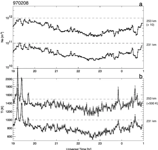
Figure 1 shows temporal variations of the electron densities (Fig. 1a) and the ion temperatures (Fig. 1b)
observed with the EISCAT radar at two F-region
heights (231 and 253 km) during the simultaneous observation period on February 8. Between 1900 and 2000 UT and 2330 and 0100 UT, the electron densities at both heights varied with ¯uctuation amplitudes of
greater than 61010 m 3 presumably due to electron
precipitation. The ion temperatures at both heights also ¯uctuated due to Joule and frictional heating. The graphs show that the large enhancements of the ion temperature (at 1912, 1922, 1940, 2349, and 0036 UT) coincided with reductions in the electron density. After the enhancements, the electron density increased imme-diately. This asymmetry between the ion temperature and the electron density can be associated with heating and electron precipitation in the vicinity of an auroral arc (Marklund, 1984). It appears that energies are deposited into the ionosphere due to Joule/frictional as well as particle heating during the geomagnetically active periods. Because the derivation of the neutral wind velocity from EISCAT radar data is less accurate during these active periods, we must be careful when
using EISCAT radar data when strong ¯uctuations in density and temperatures are observed. The electron densities and the ion temperatures from 2000 to 2330 UT showed smaller ¯uctuations than the densities and temperatures during the disturbed periods. While the electron densities showed burst enhancements at around 2030, 2102, and 2138 UT, these small ¯uctua-tions suggest that we can derive the neutral wind velocities during the quiet period more reliably.
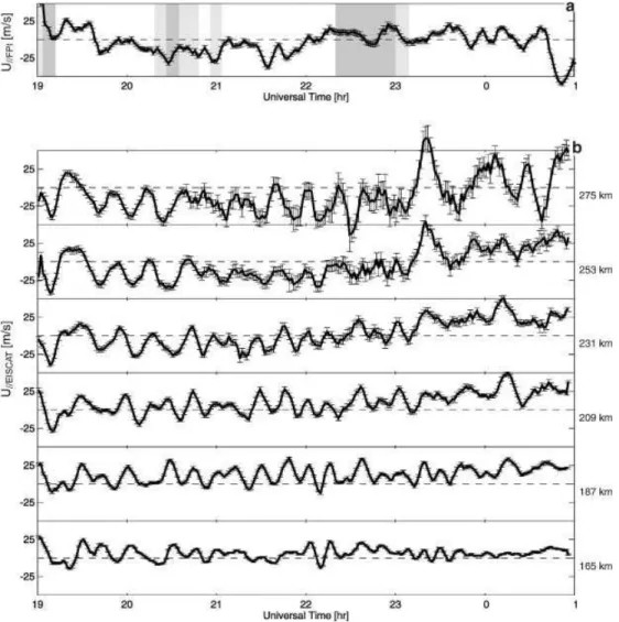
Figure 2a shows U==FPI including some data gaps. A
running-average over ®ve data points after interpolating over the gaps with a linear function was performed, so that the gaps are not visible in the curve. The periods with the gaps were shaded darker gray. The periods when the fringe radius variations, noted in Sect. 2, were remarkable were shaded lighter gray. We compared the neutral wind velocity in three periods: (A) 1912-2020 UT, (B) 2106-2218 UT, and (C) 2310-0100 UT. A positive wind is shown moving upward along the ®eld line.
Figure 2b shows U==EISCAT at altitudes from 165to
275km. EISCAT radar data from 165to 275km had no data gaps, and had relatively small ®tting errors. If the ion composition model for the IS spectrum analysis has a relatively large ambiguity for the disturbed periods,
U==EISCAT for the disturbed periods is expected to have
larger errors than for the quiet periods because the large ®tting error of EISCAT radar data introduces a higher uncertainty to the diusion velocity. However, the size of the error bars in Fig. 2b did not change greatly during the observation period. It suggests that the uncertainty of the ion composition model did not strongly aect
U==EISCAT in this height range. Using Fourier analysis,
the oscillation periods of the neutral wind velocities at these altitudes ranged from 14 to 32 min, which were longer than the Brunt-VaÈisaÈlaÈ period in this height range. Fourier analysis showed that the mean
ampli-tudes of the oscillation of U==EISCAT increased with
height. Cross-correlation analysis between U==EISCAT at
altitude of 275km and other altitudes showed height dependence of the phase (Table 1). The decrease in the time lag with height is consistent with the simulation by Kirchengast (1997). A forward phase propagation with decreasing altitude was not seen. The phase propagation
will be seen if U==EISCAT are derived at altitudes lower
than 160 km, because, in general, it becomes easy to see
with decreasing altitude. Using Fourier and cross-correlation analysis, the wave-like structures observed with the EISCAT radar are probably associated with AGWs.
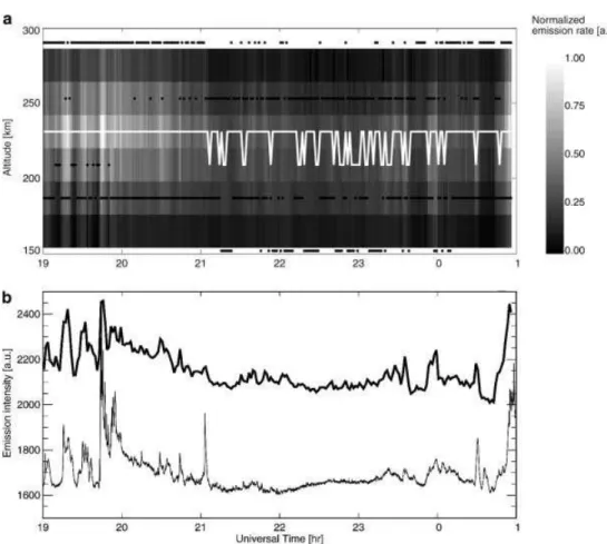
Figure 3a shows the altitude pro®le of the red-line emission rate calculated using EISCAT radar data. The emission rate was normalized by the maximum value at 1945UT at altitude of 231 km. The thick line is the altitude where the emission rate has a peak. This altitude was used to derive the neutral wind velocity for method II. The altitude of the peak emission rate was 231 km before 2100 UT. After 2100 UT, the altitude ¯uctuates between two gates, however, it is dicult to discuss the altitudinal variation of the peak emission rate from this ¯uctuation. During the observation, the altitude is expected to have been rather constant at around 231 km. The thickness of the emission layer was de®ned as the width where the emission rate is larger than 1/e of the peak value. Solid circles show the upper and lower boundaries of the emission layer. The boundaries sometimes moved below and/or above the height range, from 165to 275km, covered by EISCAT radar data in use. In that case, the solid circles were dotted out of the height range. When the upper and lower boundaries of the emission layer were within the height range, we could estimate the FPI neutral wind velocity from EISCAT radar data for method I. However, when the boundaries were out of the height range, the estimation may have had larger ambiguities on the amplitude and the phase of the neutral wind velocity from EISCAT
Fig. 3. aAltitude pro®le of red-line emission rate calculated us-ing EISCAT radar data.Thick lineshows altitude where the emission rate has a peak. The solid circlesshow the upper and lower boundaries of the emission layer, andthose out of the height range(165to 275km) show the upper or lower boundaries that are not within the height range. bThe 630.0 nm count pro®le observed with photometer along the ®eld line (thin line), and integrated emission rate over height range from 165to 275km (thick line)
Table 1. Cross-correlation coecient and time lag between
U==EISCATat altitude of 275km and at another heights for period A
Altitude (km) 165187 209 231 253
Cross-correlation coecient
0.56 0.650.70 0.850.95
radar data. The eects of the emission layer thickness on the amplitude and phase relation will be discussed in Sect. 5.
Figure 3b shows the photometer count and the emission rate integrated over the height range from 165 to 275km on the basis of the normalized rate in Fig. 3a. The photometer data are plotted every 5s by the thin line. The integrated emission rate is plotted by the thick line, which is shifted and multiplied by a factor to avoid overlapping. Cross-correlation coecient between the photometer and the derived total emission is 0.81 with the maximum showing no time lag. The relatively high value suggests that our emission model in combination with observed ionospheric data re¯ects the temporal behavior of the real emission quite accurately.
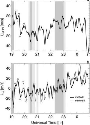
Figure 4a shows U==FPI and Fig. 4(b) shows U== I
(thick line) andU== II(thin line). The shading is the same
as in Fig. 2a. While there are discrepancies in the
amplitudes between U== I and U
II
== , both neutral winds
have similar wave-like structures.
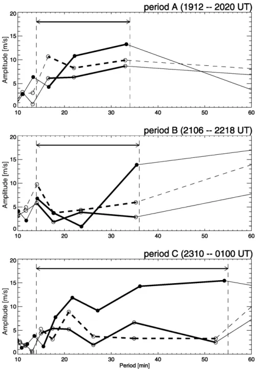
To investigate the amplitude and the phase in more
detail, we performed Fourier analysis onU== I,U== II, and
U==FPIfor periods A, B, and C. The thick lines with solid
circles in Fig. 5are the spectra ofU==FPI. The thick lines
with open circles are the spectra ofU== I, and the dashed
lines with open circles are those of U== II. The shortest
period in which we are interested is 14 min, as men-tioned in Sect. 2, and the longest one corresponds to the half length of each period: 34 min for period A, 36 min for period B, and 55 min for period C. The shortest and longest periods are marked with the vertical dashed lines. This spectrum analysis including the phase rela-tion produced the following results.
1. Oscillation period and amplitude. Table 2 shows the amplitudes which correspond to an integrated one over the selected components: 14±34 min for period A, 14±36 min for period B, and 14±55 min for period C. For
periods A and B, the amplitudes ofU== II were closer to
those of U==FPI than those of U
I
== . For period C, the
amplitudes of U== I and U
II
== were smaller than that of
U==FPI.
Figure 5shows that, for period A, the spectrum of
U== I was similar to that of U== II, though there was a
dierence in the amplitude at about 17 min. For period B, while there was also a dierence in the amplitude at
about 35min,the spectrum of U== I showed good
agree-ment with that ofU== II. These good agreements suggest
that the neutral wind velocity at around the altitude of the peak emission rate represents the velocity for method I, approximately. For period C, the amplitudes for methods I and II showed relatively large dierences at about 21 and 35min, though the amplitudes at periods of about 15and 52 min showed good agreements.
For period A, the spectra showed discrepancies in
amplitude between U==FPI and U
I
== and between U==FPI
and U== II. At about 17 min, the amplitude of U
II
== was
larger than that ofU==FPIby a factor of three. At about
22 and 33 min, the amplitudes of U== I and U== II were
smaller than that ofU==FPI. For period B, the spectra of
U== I and U II
== agreed fairly well with the spectrum of
U==FPI, except for the amplitudes at about 23 and 35min.
The three spectra had peak amplitudes at about 14 min.
For period C, the spectra ofU==FPIandU
I
== had similar
trend in amplitude from about 21 to about 35min, though there were large discrepancies in the magnitude
(by a factor of about three). The spectrum ofU==FPIand
U== II had a peak at about 21 min. A reason for the
discrepancy in amplitude will be discussed in Sect. 5as well as for the phase relation.
2. Cross-correlation and phase relation. Table 3 shows cross-correlation coecient and time lag. For period A, the cross-correlation coecients were relatively high, and the time lags were small. The signi®cance was quite
high so that oscillations ofU== IandU
II
== were thought to
synchronize with those ofU==FPI. For period B, while the
signi®cances were also quite high, the cross-correlation coecients and the time lags probably did not suggest
synchronized oscillations between U== I and U==FPI and
between U== II and U==FPI. For period C, oscillations of
U== IandU II
== were not thought to correlate with those of
U==FPI according to low cross-correlation coecients,
long time lags, and low signi®cances.
5 Discussion and conclusion
We made a comparison between the ®eld-aligned ion and neutral motions based on simultaneous EISCAT
and FPI observations. The spectra of U== I, U
II
== , and
U==FPIexpressed oscillation periods from 14 to 55 min, as
shown in Fig. 5. One dominant oscillation period is
about 14 min, which is close to the Brunt-VaÈisaÈlaÈ period
in the F-region. The observed wave-like structures in
other dominant oscillation periods appear to be internal gravity waves because the periods are above the
Brunt-VaÈisaÈlaÈ period in theF-region.
Fig. 5. Results of spectrum analysis of the ®eld-aligned neutral wind velocities shown in Fig. 4.Thick lineswithsolid circleare the spectra of the neutral wind velocity ob-served with the FPI.Thick lineswithopen circlesare the spectra of the neutral wind velocity for method I, anddashed lineswith open circlesare for method II. Thevertical dashed linesshow the shorter and longer periods used to compare the spectra: 14 and 34 min for period A, 14 and 36 min for period B, and 14 and 55 min for period C
Table 2. Integrated ampltitude ofU==FPIandU== I, andU== II over selected period components
A (m/s) B (m/s) C (m/s)
U==FPI 28 2560
U== I 21 14 26
U== II 28 23 27
Table 3. Cross-correlation coecient and time lag between U== I
andU==FPIand betweenU II
== andU==FPISigni®cance of the cross-correlation coecient is also tablated
A B C
I II I II I II
Cross-correlation coecient
0.792 0.718 0.525 0.633 0.150 0.153
There are two processes for momentum transfer between ion and neutral particles. One is momentum transfer from ions to neutrals, which takes more than
one hour in the F-region. The other is momentum
transfer from neutrals to ions, which takes only a few
seconds in the F-region. The former process makes the
neutrals oscillate with the same periods as the ions if the
ions oscillate at periods of more than one hour. U==FPI
from 1900 UT, shown in Fig. 4a, gradually shifted from upward to downward along the ®eld line, which had a
minimum value of 37 m/s at 2134 UT. The amplitude
of U==FPIthen decreased up to the end of period B. For
period C, signi®cant oscillations at a long period cannot be seen. While there were discrepancies in the amplitude,
oscillations of U== I and U
II
== were similar to those of
U==FPI. This indicates that neutral motions at periods of
longer than one hour are estimated using EISCAT radar data. This agreement is consistent with the results of comparing meridional wind velocities observed with the EISCAT radar and with the MICADO interferometer
(Thuillier et al., 1990). This similarity, however, does
not mean that the former momentum transfer process is a major in the motions at periods of longer than one hour because the latter momentum transfer process can also make ions oscillate at periods of longer than one hour if neutrals oscillate at longer periods.
In the case of the latter momentum transfer process, ions are capable of oscillating at almost the same amplitudes as the neutrals, propagating in phase with the neutrals. Thus, the latter process should produce a high cross-correlation coecient with no time lag
betweenU== I and U==FPIand betweenU
II
== andU==FPI.
For period A, the upper boundaries of the emission layer in Fig. 3a moved above the altitude of 275km most of the time. The lack of neutral wind velocity at altitudes higher than 275km results in underestimation
of amplitude of U== I because, in general, the neutral
wind amplitude increases with height in the F-region
(Witasse et al., 1998). This is because the integrated
amplitudes of U== I were smaller than the amplitude of
U==FPI, as shown in Table 2. The neutral wind velocity at
lower altitude tend to contribute to the phase of U==FPI
more signi®cantly than those at higher altitude because of a forward phase propagation with decreasing
alti-tude. For period A, U== I was thought to re¯ect all the
neutral wind motions that aected the phase relation of
U==FPI, because the lower boundaries of the emission
layer were always higher than the bottom of the height range covered by EISCAT radar data. This is because, for period A, the cross-correlation coecient was relatively high, and the time lag was relatively small, as shown in Table 3.
For periods B and C, the emission layers seem to have been thinner than those for period A, as shown in Fig. 3a. The thin layer may have expected that the
amplitude and the phase ofU== I can be close to those of
U==FPIbecause the altitudinal ambiguity in the FPI data
becomes small. The frequent expansion and down/up shifting of the emission layer, however, seem to have aected the amplitude and phase more seriously. The upper boundaries of the emission layer were sometimes
higher than the altitude of 275km, resulting in
under-estimation of the amplitude of U== I. This is consistent
with the discrepancies in the integrated amplitude in Table 2. The lower boundaries of the emission layer frequently shifted below the altitude of 165km,
result-ing in an incorrect phase relation ofU== I. This is because
the phase relations for periods B and C had relatively low cross-correlation coecients and large time lags, as shown in Table 3.
The peak-to-peak correspondence between U== I and
U==FPIand betweenU
II
== andU==FPIcan be seen in Fig. 4
for periods A, B, and C. For instance, for period A, the
oscillations ofU==FPIhad three maxima (P1, P2, and P3)
and two minima (V1 and V2). These oscillations are thought to consist of two wave structures, one with a period of about 33 min, and the other with a period of about 22 min (see top panel of Fig. 5). Similar wave
structures were also visible inU== I and U== II for period
A. These oscillation periods are shorter than that for the momentum transfer from ions to neutrals. The momen-tum transfer from neutrals to ions is thus dominant for the observed ®eld-aligned oscillations rather than the momentum transfer from ions to neutrals.
The summary of the EISCAT-FPI comparison is that
the amplitude and the phase of U==FPI have been
estimated using EISCAT radar data when the height range covered by EISCAT radar data in use has overlapped the emission layer. It is concluded that the plasma oscillations observed with the EISCAT radar at
dierent altitudes in theF-region are thought to be due
to the motion of neutrals.
Acknowledgements. The simultaneous EISCAT and FPI observa-tions were conducted under international collaboration among Norway, France, Germany, and Japan between January 11 and February 13, 1997. We are indebted to the director and sta of EISCAT for operating the facility and supplying data. We are pleased to acknowledge the considerable assistance of Dr. Hiro-taka Mori. We also would like to express our appreciation to Dr. Iwao Iwamoto. EISCAT is an international Association supported by Finland (SA), France (CNRS), The Federal Republic of Germany (MPG), Japan (NIPR), Norway (NFR), Sweden (NFR), and the United Kingdom (PPARC). This study was supported in part by the Grants-in-aid for International Scienti®c Research (09044074) and by Grants-in-aid for Scienti®c Research A (08304030) and B (08454135) from the Ministry of Education, Science, Sports and Culture, Japan. The CRL FPIs were developed for the US-Japan International Research Project to observe the middle atmosphere.
Topical Editor M. Lester thanks B. Watkins and another referee for their help in evaluating this paper.
References
Brekke, A., C. Hall, and T. L. Hansen, Auroral ionospheric conductances during disturbed conditions,Ann. Geophysicae,7, 269±280, 1989.
Forbes, J. M., F. A. Marcos, and F. Kamalabadi,Wave structures in lower thermosphere density from satellite electronics triaxial accelerometer measurements, J. Geophys. Res., 100, 14 693± 14701, 1995.
Hajkowicz, L. A., and R. D. Hunsucker,A simultaneous observa-tion of large-scale periodic TIDs in both hemispheres following an onset of auroral disturbances, Planet. Space Sci., 35,785± 791, 1987.
Hays, P. B., and S. K. Atreya, The in¯uence of thermospheric winds on the auroral red-line pro®le of atomic oxygen,Planet. Space Sci.,19,1225±1228, 1971.
Hedin, A. E.,Extension of the MSIS thermosphere model into the middle and lower atmosphere,J. Geophys. Res.,96,1159±1172, 1991.
Hedin, A. E., and H. G. Mayr, Characteristics of wavelike ¯uctuations in dynamics explorer neutral composition data, J. Geophys. Res.,92,11 159±11 172, 1987.
Hines, C. O., Internal atmospheric gravity waves at ionospheric heights,Can. J. Phys.,38,1441±1481, 1960.
Hines, C. O.,J. Atmos. Terr. Phys.,55,197±199, 1993.
Hooke, W. H., Ionospheric irregularities produced by internal atmospheric gravity waves,J. Atmos. Terr. Phys.,30,795±823, 1968.
Ishii, M., S. Okano, E. Sagawa, S. Watari, H. Mori, I. Iwamoto, and Y. Murayama,Development of Fabry-Perot interferometers for airglow observations, Proc. NIPR Symp. Upper Atmos. Phys.,10,97±108, 1997.
Kirchengast, G.,Characteristics of high-latitude TIDs from dier-ent causative mechanisms deduced by theoretical modeling, J. Geophys. Res.,102,4597±4612, 1997.
Lathuillere, C., J. Lilensten, W. Gault, and G. Thuillier,Meridional wind in the auroral thermosphere: results from EISCAT and WINDII-(O1D) coordinated measurements, J. Geophys. Res., 102,4487±4492, 1997.
Lilensten, J., G. Thuillier, C. Lathuillere, W. Kofman, V. Fauliot, and M. Herse, EISCAT-MICADO coordinated measurements of meridional wind,Ann. Geophysicae,10,603±618, 1992. Manson, A. H., C. E. Meek, and Q. Zhan,Gravity wave spectra
and direction statistics for the mesosphere as observed by MF radars in the Canadian Prairies (49N±52N) and Troms
(69N),J. Atmos. Terr. Phys.,59,993±1009, 1997.
Marklund, G., Auroral arc classi®cation scheme based on the observed arc-associated electric ®eld pattern,Planet. Space Sci., 32,193±211, 1984.
McCormac, F. G., T. L. Killeen, B. Nardi, and R. W. Smith,How close are ground-based Fabry-Perot thermospheric wind and temperature measurements to exospheric values? A simulation study,Planet. Space Sci.,35,1255±1265, 1987.
Meier, R. R., D. J. Strickland, J. H. Hecht, and A. B Christensen, Deducing composition and incident electron spectra from ground-based auroral optical measurements: a study of auroral red line processes,J. Geophys. Res.,94,13 541±13 552, 1989. Mikkelsen, I. S., T. S. Jùrgensen, M. C. Kelley, M. F. Larsen,
E. Pereira, and J. Vickrey,Neutral winds and electric ®elds in the dusk auroral oval, 1. Measurements,J. Geophys. Res.,86, 1513±1524, 1981.
Millward, G. H., R. J. Moett, S. Quegan, and T. J. Fuller-Rowell, Eects of an atmospheric gravity wave on the midlatitude ionospheric F layer,J. Geophys. Res.,98,19 173±19 179, 1993a. Millward, G. H., S. Quegan, R. J. Moett, T. J. Fuller-Rowell, and D. Rees, A modelling study of the coupled ionospheric and
thermospheric response to an enhanced high-latitude electric ®eld event,Planet. Space Sci.,41,45±56, 1993b.
Nagy, A. F., R. J. Cicerone, P. B. Hays, K. D. McWatters, J. W. Meriwether, A. E. Belon, and C. L. Rino, Simultaneous measurement of ion and neutral motions by radar and optical techniques,Radio Sci.,9,315±321, 1974.
Rees, D., N. Lloyd, P. J. Charleton, M. Carlson, J. Murdin, and I. HaÈggstroÈm, Comparison of plasma ¯ow and thermospheric circulation over northern Scandinavia using EISCAT and a Fabry-Perot interferometer,J. Atmos. Terr. Phys.,46,545±564, 1984.
Rees, M. H., and R. G. Roble, Excitation of O(1D) atoms in aurorae and emission of the [OI] 6300-AÊ line,Can. J. Phys.,64, 1608±1613, 1986.
Rice, D. D., R. D. Hunsucker, L. J. Lanzerotti, G. Crowley, P. J. S. Williams, J. D. Craven, and L. Frank, An observation of atmospheric gravity wave cause and eect during the October 1985WAGS campaign,Radio Sci.,23,919±930, 1988. Richmond, A. D., and S. Matsushita,Thermospheric response to a
magnetic substorm,J. Geophys. Res.,80,2839±2850, 1975. Sharp, W. E., M. H. Rees, and A. I. Stewart,Coordinated rocket and
satellite measurements of an auroral event 2. The rocket observations and analysis,J. Geophys. Res.,84,1977±1985, 1979. Sica, R. J., M. H. Rees, R. G. Roble, G. Hernandez, and G. J. Romick,The altitude region sampled by ground-based doppler temperature measurements of the OI 15867 K emission line in aurorae,Planet. Space Sci.,34,483±488, 1986.
Strickland, D. J., D. L. Book, T. P. Coey, and J. A. Fedder, Transport equation techniques for the deposition of auroral electrons,J. Geophys. Res.,81,2755±2764, 1976.
Strickland, D. J., R. R. Meier, J. H. Hecht, and A. B. Christensen, Deducing composition and incident electron spectra from ground-based auroral optical measurements: theory and model results,J. Geophys. Res.,94,13 527±13 539, 1989.
Taylor, M. J., and R. Edwards, Observations of short period mesospheric wave patterns: in situ or tropospheric wave generation?,Geophys. Res. Lett.,18,1337±1340, 1991. Testud, J., and P. Francois,Important of diusion processes in the
interaction between neutral waves and ionization, J. Atmos. Terr. Phys.,33,765±774, 1971.
Thuillier, G., C. Lathuillere, M. Herse, C. Senior, W. Kofman, M. L. Duboin, D. Alcayde, F. Barlier, and J. Fontanari, Co-ordinated EISCAT-MICADO interferometer measurements of neutral winds and temperatures inE- andF-regions,J. Atmos. Terr. Phys.,52,625±636, 1990.
Titheridge, J. E., Periodic disturbances in the ionosphere, J. Geophys. Res.,73,243±252, 1968.
Williams, P. J. S., T. S. Virdi, R. V. Lewis, M. Lester, A. S. Rodger, I. W. McCrea, and K. S. C. Freeman,Worldwide atmospheric gravity-wave study in the European sector 1985-1990,J. Atmos. Terr. Phys.,55,683±696, 1993.
Winser, K. J., A. D. Farmer, D. Rees, and A. Aruliah,Ion-neutral dynamics in the high latitude ionosphere: ®rst results from the INDI experiment,J. Atmos. Terr. Phys.,50,369±377, 1988. Witasse, O., J. Lilensten, C. Lathuillere, and B. Pibaret,Meridional