Article
Impact of environmental factors on maintaining water quality of
Bakreswar reservoir, India
Moitreyee Banerjee1, Joyita Mukherjee1, Arnab Banerjee1, Madhumita Roy1, Goutam Bandyopdhyay2, Santanu Ray1
1
Ecological Modeling Laboratory, Department of Zoology, SikshaBhavana, Visva-Bharati University, India
2Department of Management Studies, National Institute of Technology, Durgapur, India
E-mail: miotreyeebanerjee@gmail.com, joyitamukherjee07@gmail.com, aranya.arnab@gmail.com, yssmadhumita@gmail.com, math_gb@yahoo.co.in, sray@visva-bharati.ac.in
Received 17 March 2015; Accepted 30 April 2015; Published 1 September 2015
Abstract
Reservoirs and dams are engineered systems designed to serve purposes like supply of drinking water as well as other commercial and industrial use. A thorough assessment of water quality for these systems is thus necessary. The present study is carried out at Bakreswar reservoir, in Birbhum district, which was created by the dam, built on Bakreswar River. The major purpose of the reservoir is the supply of drinking water to the surrounding villages and Bakreswar Thermal Power Station. Water samples were collected fortnightly from three different stations of the reservoir. Physical and chemical factors like dissolved oxygen, atmospheric temperature, pH, conductivity, salinity, solar radiation, water temperature, alkalinity, hardness, chloride, productivity etc. were analysed using standard procedure. Abundance data is calculated for four major groups of zooplanktons (Cladocera, Copepoda, Ostracoda, and Rotifera) with the software PAST 2.1. Multivariate statistical analysis like PCA, hierarchical cluster and CCA are performed in order to predict the temporal variation in the water quality factors using SPSS 20. Distinct seasonal variation was found for environmental factors and zooplankton groups. Bakreswar reservoir has good assemblage of zooplankton and distinct temporal variation of environmental factors and its association with zooplankton predicts water quality condition. These results could help in formulating proper strategies for advanced water quality management and conservation of reservoir ecosystem. Key elements for growth and sustenance of the system can then be evaluated and this knowledge can be further applied for management purposes.
Keywords limnology; PCA; CCA; cluster analysis; reservoir; India.
1 Introduction
Reservoirs and dams are engineered systems designed to serve specific purpose (Kennedy, 1999). They are Computational Ecology and Software
ISSN 2220721X
URL: http://www.iaees.org/publications/journals/ces/onlineversion.asp RSS: http://www.iaees.org/publications/journals/ces/rss.xml
Email: ces@iaees.org EditorinChief: WenJun Zhang
built by impounding flowing waters. Most important functioning of the reservoir is to meet demands of the society, especially drinking water. Due to increasing pollution of aquatic ecosystems, quantity of usable water is depleting that may lead to water wars, in order to acquire safe and unpolluted water (Kennedy, 1999). Dams create new ecosystems that have hybrid characteristics of lakes and rivers (Soballe, 1992) that appear as longitudinal zones in reservoirs. Primarily reservoirs were built for irrigation purpose. Nowadays with demanding need for water in different aspects of life, reservoirs are constructed to serve multiple purposes. Water supply reservoirs are built to meet the ever increasing need for growing and upcoming industry (Straskaba and Tundisi, 1999). Even culture fishery is associated with reservoir in order to meet the growing demand of protein diet in developing and underdeveloped countries. Agricultural reservoirs are built in low plains, which allow input of turbidity causing inorganic sediments from highly-erodible soils (Geraghty, 1973). Reservoirs, being an intermediate between river and a lake have specific features that make it unique in its limnological features. Similar to a river it has longitudinal and latitudinal gradients of current velocity, width and channel depth. It also shows vertical gradients of light, temperature and dissolved oxygen which are characteristics of a lake (Cole, 1983).
According to Straskaba and Tundisi (1999) reservoir exhibit three subsystem viz. physical subsystems, chemical subsystem and biological subsystem. Water quality of a reservoir is solely dependent on the interaction of these subsystems. The food web of a reservoir consists mainly of phytoplankton, zooplankton, bacterioplankton and fish in the open water zone. The littoral zone consists of the macrophytes. Usually algae and cyanobacteria are the common phytoplankton in a reservoir. Zooplankton is an important aspect of freshwater ecosystems as it serves as a consumer of phytoplankton and is a main link in the food web (Deivanai, 2004).Today over 63,000 large (volume > 0.1 km3) reservoirs having a total surface area of approximately 400,000 km2 exist worldwide (Avakyan and Iakovleva, 1998). The incidence of dam construction was highest during the period of 1950-1980 for developed and industrial countries (Avakyan and Iakovleva, 1998). For underdeveloped and developing countries, like Asia and Africa, only 20% of the economically-feasible sites for hydroelectric power reservoir construction have been developed (Kennedy, 1999).
Thus, two aspects should be kept in mind: expanded research on managing existing water resource in developed countries and extensive advanced environmentally sound practical designs and operational strategies for developing countries. A better understanding of the interrelationship between reservoir design and operation, and limnological processes is an essential tool to reach the above mentioned aspects of water resource development (Kennedy, 1999).India is a developing country of Asia and is facing an outburst of population growth. As a result industrial and agricultural development is at full pace. Social demands for different resources are increasing fast. Thus to fulfill the necessity of water supply, reservoirs and dams are constructed throughout the country as it harbors some of world’s longest rivers. Today India has 300 dams and reservoirs approximately, and South India has the maximum number of reservoirs, especially Tamil Nadu and Karnataka.
In the present study, Bakreswar reservoir in Birbhum district is selected as a study site and environmental variables are assessed in order to get an overview of the water quality status of this reservoir. It is been reported that since the construction of this reservoir it serves as an abode to numerous migratory birds since 1999 (Sinha et al., 2012). Thus monitoring of water quality of this reservoir is necessary in order to maintain the sanctity of this precious site for winter migrants.
2 Materials and Methods
The present study is carried out in Bakreswar reservoir, Birbhum district, West Bengal (lat. 230 50.519’ N:
long. 870 24.612’ E). It was constructed on river Bakreswar as a backup water supply for the Bakreswar
Thermal Power Station under the supervision of West Bengal Power Development Corporation in 1999 (Fig. 1). But the main purpose of the reservoir is to supply drinking water to the neighboring villages of Chinpai and Bhurkuna Gram Panchayat. It is located 3 Kms northwest of the power station and has a storage volume of
2.29 million m3, retention time of 90 days and surface area of 6.38 sq. km (BKTPS project data). The reservoir
is rich in macrophytes (aquatic plant growing near water body and is either submergent, emergent or floating)
like sedge (Scirpus spp.), reed (Fragmites spp.), pond weeds (Potamogeton spp.), hornworts (Ceratophyllum
spp.), water lettuce (Enteromorpha sp., Pistia sp.), Kans grass (Saccharum spontaneum), etc (Sinha et
al.,2012). It also supports rich diversity of arthropods,molluscs and fish (Sinha and Khan, 2011). A detailed
study on the bird species revealed that it harbors breeding grounds for Great Cormorant (Phalacrocorax carbo),
Great Crested Grebe (Podiceps cristatus), Ruddy Shellduck (Tadorna ferruginea), Gadwall (Anas strepera)
and Common Coot (Fulica atra) which are considered to be indicators of Bakreswar as a wetland (Sinha and
Khan, 2011). These birds are common winter migrants which visit Bakreswar every winter (scientific names of each bird are given in parenthesis). This site is a second abode for migratory birds after the deterioration of Tilpara barrage located 17.8 km from Bakreswar and the Tilpara barrage was also considered to be the prime source of water supply to the thermal power station.
2.2 Experiments and sampling
Water samples were collected from three distinct stations of Bakreswar reservoir viz. Station I
(87025’20.9”E/33050’10.8”N), Station II (87025’13.7”E/23049’59.5’N) and Station III
(87024’9.6”E/23049’13.1”N). Samples were collected fortnightly for a period of two years from March 2012-
February 2014. For water quality analysis, 15 environmental variables like atmospheric temperature (AT),
water temperature (WT), humidity (HUM), solar irradiance (SR), water pH, dissolved oxygen (DO), salinity (SAL),
conductivity (COND), total dissolved solid (TDS), alkalinity (ALK), hardness (HARD), chloride (CHLO), total
nitrogen (TN), total phosphorous (TP) and net primary productivity (NPP) were analyzed. Water temperature
along with salinity, conductivity and total dissolved solid were calculated monthly on spot using
multi-parameter PCS testrTM35, Eutech instruments. Humidity and air temperature was recorded using
Siesedohygrotherm. Digital instruments like (LUTRON-LX 101, LUTRON-pH-206) were used to measure irradiance and pH of water respectively. Dissolved oxygen was calculated with a DO kit, Merck, Germany. For further analysis samples are filtered and preserved in 1N HCl and carried to the laboratory. Productivity of the water body was calculated through modified light and dark bottle oxygen method (Selvaraj, 2005). Chemical analysis of total alkalinity, hardness and chloride content of water was done using standard titration methods (APHA, 2005). Total nitrogen was assayed with brucine-sulphanilic acid: sulphuric acid through spectrophotometer using a standard curve (APHA, 2005). Total phosphorous was similarly calculated with ammonium molybdate: stannous chloride through spectrophotometer using a standard curve (APHA, 2005). Rainfall data was collected from Alipore Meteorological Station for the study period March 2012-Februaury 2014.
Zoolplankton samples were also collected fortnightly for two consecutive years in 50 ml sample bottles and preserved with 4% formalin on spot. About 30 L of water was passed through a zoolplankton net of mesh size 200µ during each sampling. Samples were brought to the laboratory and four major zooplankton groups i.e. Cladocera, Copepoda, Ostracoda and Rotifera were counted in Sedgewick Rafter Counter to enumerate the monthly density (no/L). Cladocerans (also called water fleas) are a small group of arthropods belonging to the order Cladocera. The common features are presence of compound eye and a carapace covering the thorax. Copepods are also small crustaceans having tear shapes body with large antennae and telson at the posterior end of the body. Ostracods are similar crustaceans with body encased in a bivalve shell. Rotifers are separate group of zooplankton with distinct corona at the head region.
2.3 Statistical enumeration
Correlation and multivariate analysis of variance (MANOVA) was done in order to predict the interrelationship between different studied environmental variables, as also their seasonal variation. This was
done using software S-PLUS 4.0. Environmental characteristics are multivariate variables and thus methods of
relationship of considered environmental variables and zooplankton functional groups. Both clustering and CCA was done using SPSS 20, IBM Corp, 2011 and PAST version 2.10 (Hammer, 2001) respectively.
3 Results
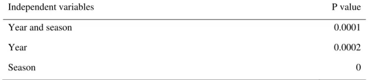
At first, year and season are taken as two independent variables and the environmental variables and plankton density are considered as dependent variables. Results show a significant effect, where as when year and season are considered separately as independent variable for MANOVA, season have high significant effect on the environmental variables as well as zooplankton density (Table 1).
Table 1 P values for MANOVA done to show effects of seasons and year on different environmental variables.
Independent variables P value
Year and season 0.0001
Year 0.0002
Season 0
Correlation analysis has been done to understand the inter-relation among the different environmental factors for the period March 2012-February 2013 and March 2013-February 2014. Out of all the environmental variables studied that are good indicators of water quality, high correlation is found between eight variables for the year 2012-2013 and 2013-2014 (Table 1 and 2).
Table 2 Correlation values for the period March 2012-February 2013.
AT HUM SR WT COND SAL TDS HARD
AT 1 -0.110 0.444** 0.858** -0.039 -0.204 -0.160 -0.040
HUM -0.110 1 -0.611** 0.309** -0.438 .000 0.086 0.164
SR 0.444** -0.611** 1 0.091 0.227 -0.150 -0.217 -0.183
WT .858** .309** .091 1 -.190 -.189 -.089 .028
COND -0.039 -0.438 0.227 -0.190 1 0.514** 0.489** 0.219
SAL -0.204 .000 -0.150 -0.189 0.514** 1 0.759** 0.653**
TDS -0.160 0.086 -0.217 -0.089 0.489** 0.759** 1 0.586**
HARD -0.040 0.164 -0.183 0.028 0.219 0.653** 0.586** 1
**significant at 0.01 level.
Correlation values for the period 2012-2013 shows that AT and WT shows a positive inter-correlation,
whereas HUM and SR shows a negative inter-correlation. Similarly COND, SAL, TDS and HARD are highly
with AT and WT showing strong positive inter-correlation, whereas HUM and SR showing negative
inter-correlation. Correlation values between COND, SAL, TDS and HARD shows more strong positive correlation
compared to previous study period (Table 3).
Table 3 Correlation values for the period March 2013-February 2014.
AT HUM SR WT COND SAL TDS HARD
AT 1 -0.059 0.385** 0.927** 0.089 0.196 0.021 0.091
HUM -0.059 1 -0.428** 0.199 -0.181 -0.162 -0.198 -0.149
SR 0.385** -0.428** 1 0.160 -0.047 -0.012 -0.079 0.013
WT 0.927** 0.199 0.160 1 0.003 0.131 -0.060 0.003
COND 0.089 -0.181 -0.047 0.003 1 0.943** 0.907** 0.525**
SAL 0.196 -0.162 -0.012 0.131 0.943** 1 0.902** 0.552**
TDS 0.021 -0.198 -0.079 -0.060 0.907** 0.902** 1 0.510**
HARD 0.091 -0.149 0.013 0.003 0.525** 0.552** 0.510** 1
**significant at 0.01 level.
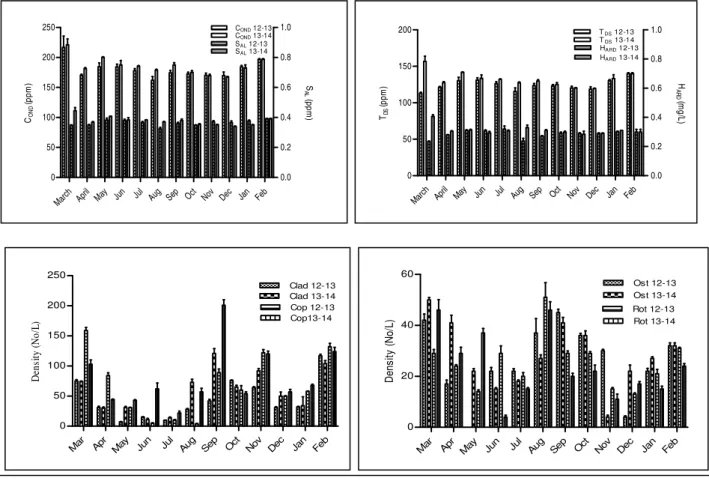
MANOVA have showed seasonality in the variation pattern of environmental variables as well as zooplankton functional groups. Temperature gradually increases from spring, to highest during monsoon and gradually decreases in winter. Similarly as solar irradiance increases in summer humidity remains low, the latter gradually reaching its maximum during the monsoon when solar irradiance is low. The minerals remain high during the summer months and are low during monsoon and winter. Zooplankton functional groups show two distinct peaks; one at the onset of spring (Feb-Mar) and the other in monsoon (Jul-Sep) (Fig. 2). Annual precipitations of two consecutive years are presented in Fig. 3.
March Ap ril
May Jun Jul Aug Sep Oct Nov Dec Jan Feb 0
10 20 30 40
0.0 0.2 0.4 0.6 0.8 1.0
WT 12-13
WT 13-14
AT 12-13
AT 13-14
WT TA
Marc h
April May Jun Jul Aug Sep Oct Nov Dec Jan Feb 0
200 400 600
0.0 0.2 0.4 0.6 0.8 1.0
HUM 12-13
HUM 13-14
SR 12-13
SR 13-14
HUM
(%
) RS (
Lux
Based on the correlation values, eight environmental variables are considered for centered PCA ordination. In both years total variance explained for the said variables accounts for 82.73% and 84.44% for the study period 2012-2013 and 2013-2014 respectively. The rotated component matrix following Varimax method with Kaiser Normalization also projected same component extraction for the study period (Table 4 and 5). Rotated component matrix shows that maximum variance is contributed by 4 variables which include conductivity, salinity, total dissolved solid and hardness which comprises the first component. Atmospheric and water temperature contributes to the next level of variation and belongs to component 2. The rest variation
Marc h
April May Jun Jul Aug Sep Oct Nov Dec Jan Feb 0 50 100 150 200 250 0.0 0.2 0.4 0.6 0.8 1.0
COND 12-13 COND 13-14
SAL 12-13
SAL 13-14
CON D (p p m ) S AL (p p m ) Mar ch
April May Jun Jul Aug Sep Oct Nov Dec Jan Feb 0 50 100 150 200 0.0 0.2 0.4 0.6 0.8 1.0
TDS 12-13 TDS 13-14 HARD 12-13 HARD 13-14
TDS
(p
pm
) ARH
D (m g /L ) Ma r
Apr May Jun Ju l
Aug Sep Oct Nov Dec Jan Feb 0 50 100 150 200 250 Clad 12-13 Clad 13-14 Cop 12-13 Cop13-14 D ens it y (N o/ L)
Mar Apr May Jun Jul Aug Sep Oct Nov Dec Jan Feb 0 20 40 60 Ost 12-13 Ost 13-14 Rot 12-13 Rot 13-14 D ens it y ( N o/ L)
Fig. 2 Annual variation of environmental variables and Zooplankton groups a) AT & WT b) HUM & S c) COND & SAL d) TDS &
HARD e) Cladocera (Clad) & Copepoda (Cop) f) Ostracoda (Ost) & Rotifera (Rot).
Fig. 3 Annual rainfall for two consecutive study periods
Mar Apr May Jun Jul Aug Sep Oct Nov Dec Jan Feb
pattern among the variables is contributed by humidity and solar irradiance belonging to component 3.
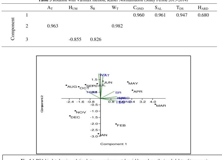
A PCA bi-plot (Figure 4) is made to analyze the variation pattern of the studied variables through seasons. Maximum variation in air and water temperature along with humidity occurs during monsoon i.e. June-September. Water minerals and solar irradianceshow variation during the summer i.e. March-May. The central idea of principal component analysis (PCA) is to reduce the dimensionality of a data set consisting of a large number of interrelated variables, while retaining as much as possible of the variation present in the data set (Joliffe, 2002). This was successfully done in the present study for the study period 2012-2013 and 2013-2014. It has clearly reduced the entire data set into three principal components completely partitioning the variables based on their similar variance pattern and also accounted for more than 82% of total variance explained during PCA. The PCA bi-plot (Fig. 4) showed that March-May, the pre-monsoon months, experienced maximum variation in all forms of minerals dissolved in water. The month of monsoon experienced variation in temperature of air and water, along with humidity and solar irradiance.
Table 4Rotation with Varimax method, Kaiser Normalisation (Study Period 2012-2013)
AT HUM SR WT COND SAL TDS HARD
Component
1 0.595 0.907 0.893 0.799
2 0.950 0.959
3 -0.909 0.816
Table 5 Rotation with Varimax method, Kaiser Normalisation (Study Period 2013-2014)
AT HUM SR WT COND SAL TDS HARD
Component
1 0.960 0.961 0.947 0.680
2 0.963 0.982
3 -0.855 0.826
AT
HUM SR
WT
COND SAL TDS
HARD
MAR APR
MAY JUN
JUL
AUG SEP
OCT
NOV
DEC
JAN
FEB
-2.4 -1.6 -0.8 0.8 1.6 2.4 3.2 4.0
Component 1 -3.0
-2.5 -2.0 -1.5 -1.0 -0.5 0.5 1.0 1.5
C
om
ponen
t 2
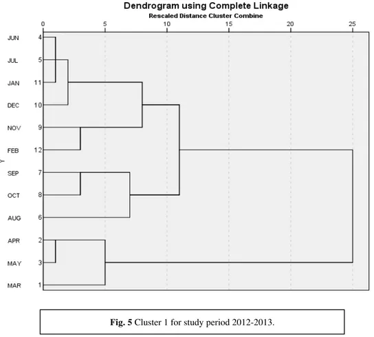
Cluster analysis of the study period showed a more or less similar pattern.Hierarchical cluster predicted three preliminary clusters pooling the months on their similarity in environmental factors. Cluster 1(Fig.5) is based on data of study period 2012-2013. It reflects that summer months (March- May) forms a primary cluster, the winter months forms a second primary cluster, but the months June and July are also included in it. The late monsoon months i.e. Aug-Oct forms another primary cluster. The winter and the late monsoon months together form the secondary cluster which is joined to the summer cluster. Cluster 2 (Fig. 6) is based on study period 2013-2014. It also shows three primary clusters, the only difference is that monsoon cluster comprises of months June-September. Thus year two shows distinct seasonal clustering based on similarities in environmental factors. Canonical Correspondence analysis shows an intricate relationship between the
environmental variables and zooplankton group abundance. The first two CCA axes (Axis I with = 0.0621
and Axis II with =0.0171) showed 76.74% variance in the zooplankton abundance data. Environmental
variables are represented by trajectories and point the factor direction for maximum variation. Importance of
each variable in assemblage ordination is predicted by the length of the trajectory (Fig. 7). Thus AT, WT,
followed by HARD, CHLO, ALK, N and P have significant effect on zooplankton abundance. The rest variables
have less effect on zooplankton.
AT
HUM SR
WT COND
SAL
TDS
HARD
pH DO
ALK
Chlo N
P
Cladocera Copepoda
Ostracoda
Rotifera
-2.0 -1.5 -1.0 -0.5 0.0 0.5 1.0 1.5 2.0 2.5
Axis 1 -2.0
-1.6 -1.2 -0.8 -0.4 0.0 0.4 0.8 1.2 1.6
Ax
is
2
Fig. 6 Cluster 2 for study period 2013-2014.
4 Discussion
India is a tropical country and seasonal partitioning of Southern Bengal is mainly based on rainfall in this region. Accordingly monsoon sets from mid Jun-September, followed by winter that starts from November and persists till February. The dry season or pre monsoon is usually of three months, March-May. Environmental variables as well as zooplankton density of Bakreswar reservoir varied seasonally as depicted in Fig. 2. Even results of MANOVA showed a significant effect of season on zooplankton density (Table 1). Copepods and Cladocerans were highest during the months of August and February-March. Rotifers were found to be abundant during the late summer months, so were the Ostracods. Similar seasonal fluctuations were also reported from reservoirs of other states of India (Ahmed et al., 2013; Jadhav, 2012). Temperature has a positive effect on the rotifer abundance as established by Smith (1983). Annual seasonal variations of cladoceran populations in Indian aquatic bodies were also established in the works of Mathew (1985) and Rao et al. (1981). Works of Shivshankar (2013) and Rajashekhar (2012) from Southern reservoirs of India also confirms such observations as found in Bakreswar reservoir.
The results of correlation analysis show that physical and chemical factors of the reservoir are highly correlated to each other. It is also seen that variation for environmental factors is highly significant through seasons and year. Seasonal variation pattern is quite common for all aquatic system. In this study there is also significant variation in the studied variables. One possible explanation to this can be attributed to the variation in rainfall between the two study periods (Fig. 4). During 2012-13, onset of precipitation was late which caused the summer months to prevail for a long time causing an increase in minerals due to over evaporation. But in 2013-14, monsoon was early in the month of June thus causing excessive rain which extended till the end of August. As a result mineral components of the reservoir got diluted and settled in the water body.
Variation in monthly rainfall is also related to SR and HUM. Mineral components of any reservoir water are
summarized by its TDS, COND, HARD, ALK and SAL (Soballe, 1992). Singh et al. (2004), while analyzing the
temporal variation of water quality in riverine system also concluded that minerals are the essential components of any aquatic ecosystem. On the other hand, Tarkan (2010) studied different water quality factors and suggested that physical factors like temperature, light intensity, depth etc are the primary factors
responsible for temporal variation in reservoir ecosystem, whereas chemical components like TDS, chloride,
alkalinity are secondary factors.
Centered PCA ordination shows that the entire data set is extracted into three components based on their total variance pattern. The results of PCA of present study show that minerals form the principal component
(51.23 % of total variance) controlling the reservoir water quality, followed by temperature (AT and WT) and
humidity: solar radiance inter-relation. A study from river basin in Florida, USA showed that minerals are essential important factors for assessing water quality in aquatic systems (Quyang, 2005). This is also elucidated in the works of Singh et al. (2004). But one cannot ignore the effect of physical factors in temporal variation of water quality in the studied reservoir as the second and third component (Table 4 and 5) accounted for 26.62% and 15.05% of the total variation.
Bakreswar reservoir is rocky and sandy, but as more water recedes, the substratum becomes muddy. It is
suggested that TDS, COND, HARD remains high in dry season due to high rate of evaporation and shallow water
depth (Hujare, 2008; Tarkan, 2010 and Medudhula 2012). A similar study from Fuji river basin, Japan also showed that principal factors related to water quality of that riverine system are conductivity, temperature and other nutrients (Shrestha, 2007).
With the onset of monsoon, water column increases gradually to a depth of 75m; as a result mineral components gradually decrease and settle at a standard range. It is also suggested that onset of summer causes
a gradual increase in COND, TDS and HARD which gradually settles to a normal range during monsoon due to
excessive dilution (Bengrain and Marhaba, 2003).Due to cloudy condition the light intensity also decreases. But gradual increase in precipitation increases the humidity of this region. Temperature is an important factor, which regulates the biogeochemical activities in aquatic environment (Sivakumar, 2008). Air temperature remains high during monsoon as it is not affected by precipitation. This in turn controls the surface water temperature of the reservoir (Gupta and Sharma, 1993; Garg et al., 2010; Agarwal and Rajwar, 2010).
Cluster analysis encompasses a wide range of techniques for exploratory data analysis (Razmkhah, 2010). The main aim of CA is grouping objects (cases) into classes (clusters) so that objects within a class are similar to each other but different from those in other classes. In cluster analysis, the objects are grouped by linking inter-sample similarities and the outcome illustrates the overall similarity of variables in the data set (Massart and Kaufman, 1983). During the study period 2012-2013, monthly cluster based on similarities in environmental factors, show that early monsoon months (June-July) are remotely related to the winter cluster, but during 2013-2014 a separate cluster is formed comprising of early and late monsoon months. This variation is due to a change in precipitation in these two consecutive years. During 2012-2013, monsoon came late than the normal time and also continued till the end of October, whereas during 2013-2014, onset of monsoon is from June and continued till September. A case study from Tigris river basin, Turkey formed two clusters (wet and dry) from a 12 month data set of physico-chemical factors base on their seasonal similarity (Varol et al., 2012).
The canonical correspondence analysis predicts the occurrence or abundance of biotic data on an environment gradient (terBraak, 1995). The occurrence of organisms usually depends on the weighted average of the environmental factors. Usually temperature, minerals, nutrients and dissolved oxygen are the prime determinant of zooplankton abundance as predicted by Dejen et al., (2004). In estuarine system salinity is considered to be the important environmental gradient for zooplankton distribution (Soetaert, 1993; Albaina, 2009). In the present study it is found that Ostracods and Rotifers are mainly dependent on the temperature, minerals and nutrient condition of the reservoir, copepods are influenced by dissolved oxygen and salinity,
whereas pH and TDS has a direct effect on cladocerans. The effect of copepods was establishedin the works of
Sellami (2011). Rotifer was found to be negatively correlated to Axis 2 and thus it can be said that temperature, nitrate and pH has a negative effect on rotifer assemblage. Such case is also reported from NathSagar Reservoir, Madhya Pradesh (Pradhan, 2011). In Indian reservoirs temperature play an important role in zooplankton assemblage as suggested by Goerge et al. (1961). Thus water quality of the reservoir depends on temporal variation of physic-chemical factors which in turn controls the zooplankton abundance seasonal variation in the studied reservoir.
5 Conclusion
Bakreswar reservoir shows significant temporal variation in both environmental factors and zooplankton abundance. The essential factors controlling the water quality of the reservoir were minerals, temperature and solar irradiance: humidity ratio. All these in turn control the temporal zooplankton variation as revealed from multivariate statistical analysis. Distinct seasonal patterning is revealed through cluster analysis. To sum up it can be said that Bakreswar reservoir has a good environmental condition with periodic zooplankton assemblage and the water quality of the reservoir are within the limits of drinking water standards.
Acknowledgement
The author MB would like to acknowledge Head, Department of Conservation Biology, Durgapur Govt. College for the necessary help regarding the spectrophotometric analysis. More sincere thanks to Krishna Bhakat, field assistant for the help provided during sampling and field data collection. MB carried out the entire field sampling for two years in the study site. MB, JM and GB carried out the data and statistical analysis for the said work. AB and MR helped in manuscript preparation especially the figures. SR conceived the experimental design, manuscript preparation and correction.
References
Agarwal AK, Rajwar GS. 2010. Physico-chemical and microbiological study of Tehri Dam Reservoir, Garhwal Himalaya, India. Journal of American Science, 6(6): 65-71
Ahmad Y, Hussain A, Hussain G, Tharani M, Amine Md. 2013. Diversity and seasonal variations of zooplanktons in Pahuj Reservoir at Jhansi (UP) India. International Journal of Pharmaceutical and Biological Achieve, 4(1): 100-104
Albaina A, Villate F, Uriarte I. 2001. Zooplankton communities in two contrasting Basque estuaries (1999– 2001): reporting changes associated with ecosystem health. Journal of Plant Research, 1(1): 1-14
APHA AWWF and WEF. 2005. Standard methods for the examination of water and
wastewater.21stedn.American Public Health Association, Washington DC, USA
Avakyan J, Iakovleva VB. 1998. Status of global reservoirs: the position in the late twentieth century. Lakes and Reservoirs.Research and Management 3: 45-52
Bakreswar Thermal Power Project (1) & (2). West Bengal Power Development Corporation. 1-19, India Bengra¨ıne K Marhaba TF. 2003. Using principal component analysis to monitor spatial and temporal changes
in water quality. Journal of Hazardous Material, B100: 179-195
Chessel D, Lebreton JD, Yoccoz N. 1987. Propri6t6s de l'analysecanonique des correspondances; une illustration en hydrobiologie. Annual Review of Statistics and Its Application, 35:55-72
Cole GA. 1983. Textbook of Limnology (3rd edn). Waveland Press, USA
Deivanai K, Arunprasath S, Rajan MK, Baskaran S. 2004. Biodiversity of phytoplankton and zooplankton in relation to water quality parameters in a sewage polluted pond at Ellayirampannai, Virudhunagar District. In: The Proceedings of National Symposium on Biodiversity Resources Management and Ustainable Use. Centre for Biodiversity and Forest studies, Madurai Kamaraj University, Madurai, India
Dejen E, Vijverberg J, Nagelkerke LAJ, Sibbing FA. 2004. Temporal and spatial distribution of
microcrustacean zooplankton in relation to turbidity and other environmental factors in a large tropical lake (L. Tana, Ethiopia). Hydrobiology, 513: 39-49
61-76
Geraghty JJ, Miller DW, Van Der Leeden F, Troise FL. 1973. Water Atlas of the United States. A Water Center Publication, Port Washington, NY, USA
George MG 1961. Observation on the rotifers from shallow ponds in Delhi. Current Science, 30: 26-268 Gupta MC, Sharma,LL. 1993. Diel variations in selected water quality parameters and zooplankton in a
shallow pond of Udaipur, Rajasthan. Journal of Ecobiology, 5: 139-142
Hammer Ø, Harper DAT, Ryan PD. 2001. PAST: Paleontological statistics software package for education and data analysis. Palaeontol Electron, 4(1): 9
Hujare MS. 2008. Seasonal variations of phytoplankton in the freshwater tank of Talsande, Maharashtra. Nature Environ & Poll. Tech., 7(2): 253-256
Jadhav S, Borde S, Jadhav D, Humbe A. 2012. Seasonal variations of zooplankton community in SinaKolegoan Dam Osmanabad district, Maharashtra, India. Journal of Experimental Sciences, 3(5): 19-22
Joliffe IT. 2002. Principal Component Analysis (2nd edn). 2-3, Springer, Germany
Kennedy RH. 1999. Reservoir Design and Operation: Limnological Implications and Management Oppurtunities. In: Theoretical Reservoir Ecology and its Applications (Tundisi JG, Straskaba M, eds). Backhuys, Leiden, Netherlands
Legendre P, Legendre L. 2003. Numerical Ecology (2nd English edition.Elsevier, Netherlands
Leps J, Straskaba M, Desortova B, Prochaszkova L. 1990. Annual cycles of plankton species composition and physical chemical conditions in Slapy Reservoir detected by multivariate analysis. Archiv für Hydrobiologie, 3: 934-945
Massart DL, Kaufman L. 1983. The Interpretation of Analytical Chemical Data by the Use of Cluster Analysis. Wiley, New York, USA
Mathew PM. 1985. Seasonal trends in the fluctuations of plankton and physic-chemical factors in a tropical lake (Govingarh lake, M.P.) and their interrelationships. Journal of Inland Fisheries Society India, 17(1&2): 11-24
Medudhula T, Samatha Ch, Sammaiah C. 2012. Analysis of water quality using physico-chemical parameters in lower manair reservoir of Karimnagar district, Andhra Pradesh. International Journal of Environmental Science, 3(1): 172-180
Odum ER. 1971. Fundamentals of Ecology.3rd Edition, WB Saunders Company, Philadelphia, USA
Ouyang Y. 2005. Evaluation of river water quality monitoring stations by principal component analysis. Water Research, 39: 2621-2635
Pradhan V, Patel R, Bansode SG. 2011. Biodiversity of population dynamics and seasonal variation in NathSagar Reservoir at Paithan (M.S) India, with reference to Rotifiers. International Journal of Science Innovations and Discoveries, 1(3): 320-326
Rajashekhar M, Vijaykumar K, Paerveen Z. 2010. Seasonal variations of zooplankton community in freshwater reservoir Gulbarga District, Karnataka, South India. International Journal of Systems Biology, 2(1): 6-11
Rao M, Mukhopadhyay B, Moley EV. 1981. Seasonal and species of zooplanktonic organisms and theirsuccession in two freshwater ponds at Wagholi, Poona. Proceedings of the Symposium on Ecology of Animal Populations Zoological Survey of India, 2: 63-84
Sellami I, Elloumi J, Hamza A, Mohammed AM, Ayadi H. 2011. Local and regional factors influencing zooplankton communities in the connected Kasseb Reservoir, Tunisia. 37(2): 201-212
Selvaraj GSD. 2005. Estimationof primary productivity (modified light and dark bottle oxygen
method).CMFRI Special Publication Mangrove ecosystems: A Manual for The Assessment of Biodiversity, 83: 199-200
Shivashankar P, Venkataramana GV. 2013. Zooplankton diversity and their seasonal variations of Bhadra Reservoir, Karnataka, India. International Research Journal of Environment Science, 2(5): 87-91
Shrestha S, Kazama F. 2007. Assessment of surface water quality using multivariate statistical techniques: A case study of the Fuji river basin, Japan. Environmental Modelling and Software, 22: 464-475
Singh KP, Malik A, Mohan D, Sinha S. 2004. Multivariate statistical techniques for the evaluation of spatial and temporal variations in water quality of Gomti River (India)—a case study. Water Research, 38: 3980–3992
Sinha A, Hazra P, Khan TN. 2011. Population trends and spatiotemporal changes to the community structure of waterbirds in Birbhum District, West Bengal, India. Proceedings of Zoological Society, 64: 96-108 Sinha A, Hazra P, Khan TN. 2012. Emergence of a wetland with the potential for an avian abode of global
significance in South Bengal, India. Current Science, 102(4): 613-616
Sivakumar K, Karuppasamy R. 2008. Factors affecting productivity of phytoplankton in a reservoir of Tamilnadu, India. American-Eurasian Journal of Botany, 1(3): 99-103
Smith VH. 1983. Low nitrogen to phosphorus ratio favour dominance by blue green algae in lake phytoplankton. Science, 221: 669-671
Soballe DM, Kimmel BL, Kennedy RH, Gaugush RF. 1992. Reservoirs. In: Hackney CT, Adams SM, Martin WH Biodiversity of the southeastern United States: Aquatic Communities. 421-474, Wiley, New York, USA
Soetaert K, Rijswijk P.Van. 1993. Spatial and temporal patterns of the zooplankton in the Westerschelde estuary. Marine Ecological Progress Series, 97: 47-59
Straskraba M, Tundisi JG. 1999. Guidelines of Lake Management.Vol 9. Reservoir Water Quality Management, Internternational Lake Environment Community, Japan
Tarkan AS. 2010. Effects of Streams on drinkable water reservoir: An assessment of water quality, physical habitat and some biological features of the streams. Journal of Fisheries Science, 4(1): 8-19
terBraak CJF, Verdonschot Piet EM. 1995. Canonical correspondence analysis and related multivariate methods in aquatic ecology. Aquatic Sciences, 57(3): 255-289
terBraak CJF. 1986. Canonical correspondence analysis: a new eigenvector technique for multivariate direct gradient analysis. Ecology, 67:1167-1179
terBraak CJF. 1987a. The analysis of vegetation-environment relationships by canonical correspondence analysis.Vegetation, 69: 69-77
terBraak CJF. Ordination. In: Jongman RHG, terBraak CJE, van Tongeren OER. 1987b. Data Analysis in Communityy And Landscape Ecology, Pudoc, Wageningen (reprinted by Cambridge University Press, Cambridge, 1995), 91-173
Varol M, Gokot B, Beklyan A, Sen B. 2012. Spatial and temporal variations in surface water quality of the dam reservoirs in the Tigris River basin, Turkey. Catena, 92: 11-21