HLAODV – A Cross Layer Routing Protocol for
Pervasive Heterogeneous Wireless Sensor
Networks Based On Location
Jasmine Norman1 , J.Paulraj Joseph2
1
Vellore Institute of Technology, Chennai – 14, India
2
Manonmaniam Sundaranar University, Tirunelveli-12, India
Abstract
A pervasive network consists of heterogeneous devices with different computing, storage, mobility and connectivity properties working together to solve real-world problems. The emergence of wireless sensor networks has enabled new classes of applications in pervasive world that benefit a large number of fields. Routing in wireless sensor networks is a demanding task. This demand has led to a number of routing protocols which efficiently utilize the limited resources available at the sensor nodes. Most of these protocols either support stationary sensor networks or mobile networks. This paper proposes an energy efficient routing protocol for heterogeneous sensor networks with the goal of finding the nearest base station or sink node. Hence the problem of routing is reduced to finding the nearest base station problem in heterogeneous networks. The protocol HLAODV when compared with popular routing protocols AODV and DSR is energy efficient. Also the mathematical model of the proposed system and its properties are studied.
Keywords: Pervasive, Sensor, Heterogeneous, Routing, Location
1. Introduction
Pervasive Computing is a technology that pervades the users’ environment by making use of multiple independent information devices (both fixed and mobile, homogeneous or heterogeneous) interconnected seamlessly through wireless or wired computer communication networks which are aimed to provide a class of computing / sensory / communication services to a class of users, preferably transparently and can provide
personalized services while ensuring a fair degree of privacy / non-intrusiveness. The goal of pervasive computing is to create ambient- intelligence, reliable connectivity, and secure and ubiquitous services in order to adapt to the associated context and activity. To make this envision a reality, various interconnected sensor networks have to be set up to collect context information, providing context-aware pervasive computing with adaptive capacity to dynamically changing environment. Wireless sensor networks (WSN) can help people to be aware of a lot of particular and reliable information anytime anywhere by monitoring, sensing, collecting and processing the information of various environments and scattered objects [24]. The flexibility, fault tolerance, high sensing, self-organization, fidelity, low-cost and rapid deployment characteristics of sensor networks are ideal to many new and exciting application areas such as military, environment monitoring, intelligent control, traffic management, medical treatment, manufacture industry, antiterrorism and so on [18,23]. Therefore, recent years have witnessed the rapid development of WSNs. In this paper, we address the issue of cross-layer networking for the pervasive networks , where the physical and MAC layer knowledge of the wireless medium is shared with network layer, in order to provide efficient routing scheme to prolong the network life time.
large scale of deployment and unattended operation. The challenges of WSN have been studied by Yao K [29]. The key challenge in wireless sensor networks is maximizing network lifetime. Routing for WSNs is one of the most active research areas. Energy efficiency and network capacity are perhaps two of the most important issues in wireless ad hoc networks and sensor networks. Many to one communication paradigm is widely used in regard to sensor networks since sensor nodes send their data to a common sink for processing. This many-to-one paradigm also results in non-uniform energy drainage in the network.
Sensor networks can be divided in to two classes as event driven and continuous dissemination networks according to the periodicity of communication. In event-driven networks, data is sent whenever an event occurs. In continuous dissemination networks, every node periodically sends data to the sink. Routing protocols are usually implemented to support one class of network in order to save energy. Almost all the research involved with routing is related to sending the sensed data to a control center or to a fixed destination. This paper argues that the problem of routing can be reduced to sending the data to the nearest base station, as the base station will have the capacity to directly deliver the data to the control center, to which the sensor is attached to. This not only will reduce the time delay but also will be energy efficient.
The assumption of homogeneous nodes does not always hold in practice since even devices of the same type may have slightly different maximal transmission power. There also exist heterogeneous wireless networks in which devices have dramatically different capabilities, for instance, the communication network in the Future Combat System which involves wireless devices on soldiers, vehicles and UAVs. In contrast to a traditional static wireless sensor network which consists of a large number of small sensor nodes with low computational, storage and communication capabilities, such limitations no longer apply in a mobile sensor network. In [27] the use of vehicles as sensors in a “vehicular sensor network,” a new network paradigm that is critical for gathering valuable information in urban environments is studied. However, existing routing protocols for WSNs are built on the network architecture (called flat architecture) such that all sensor nodes are homogeneous and send their data to a single sink
node by multiple hops [3,5,15,21]. Such a flat architecture is inapplicable to many real applications with large-scale and heterogeneous sensor nodes.
A typical network configuration consists of sensors working unattended and transmitting their observation values to some processing or control center, the so-called sink node, which serves as a user interface. Due to the limited transmission range, sensors that are far away from the sink deliver their data through multihop communications, i.e., using intermediate nodes as relays. The given scheme is based on probabilities. The probability as relay node is high for the base station, medium for the mobile sensors and very low for the stationary sensors. Thus the stationary sensors are less likely to be selected as a hop for the relay of information. Deterministic choices based on heavy collection of information into the message are replaced by probabilistic choices by using classical optimization heuristics. We also modeled the heterogeneous network as a random geometric graph and studied the properties.
In this paper, we present a new event driven routing protocol for the pervasive heterogeneous networks which prolongs the life time of the network by considering type of nodes. Simulation results show that our protocol outperforms the traditional routing approaches in terms of network lifetime and latency and is more suitable for real world applications. The remainder of the paper is organized as follows. Section II provides a brief overview of the related work. Section III explains the operation of the new routing protocol. Section IV gives the mathematical model of the system. Section V compares the performance of HLAODV and the protocols used in traditional schemes. Section VI provides the conclusion of the work and discusses future directions.
2.
Related Work
stack in an attempt to optimize the use of their scarce resources. In particular, the routing problem, has received a great deal of interest from the research community with a great number of proposals being made. In [ 8] L.Chen et al have studied a cross layer design for routing in ad hoc wireless networks. Basically the existing protocols can be fit in one of two major categories: on-demand such as AODV [21] and DSR [15], and proactive such as DSDV [22] and OLSR [9]. The review of these protocols is found in [4, 14]. Ad hoc on-demand distance vector (AODV) routing [21] adopts both a modified on-demand broadcast route discovery approach used in DSR [15] and the concept of destination sequence number adopted from destination-sequenced distance-vector routing (DSDV)[22]. Directed diffusion [13] is a good candidate for robust multi hop multi path routing and delivery. This enables diffusion to achieve energy savings by selecting empirically good paths and by caching and processing data in-network (e.g., data aggregation). The authors in [2, 10] have analyzed the performance of the popular protocols after classification. The common belief is that a multi-hop configuration with rather small per-hop distance is the only viable energy efficient option for wireless sensor networks. [3,5,25] have studied the various options for energy efficient wireless sensor network.
Location-based algorithms [16,17,31] rely on the use of nodes position information to find and forward data towards a destination in a specific network region. Position information is usually obtained from GPS (Global Positioning System) equipment. They usually enable the best route to be selected, reduce energy consumption and optimize the whole network. In [18] Ye Ming Luz et al have proposed location based energy efficient protocol. Na Wang et al in [19] have studied the performance of the probabilistic multi path geographic based protocols. In [32] position-based routing protocols are surveyed and classified into four categories: flooding-based, curve-flooding-based, grid-based and ant algorithm-based.
There is very less research work done related to heterogeneous sensor networks. The integration of different wireless access technologies combined with the huge characteristic diversity of supported services in next-generation wireless systems creates a real heterogeneous network. Authors in [12] have
proposed a secure routing protocol for heterogeneous sensor networks. In [1] the authors proposed a generic practical framework that optimizes media streaming in heterogeneous systems by taking advantage of cost and resource characteristic diversity of the integrated access technologies and the buffering capability of streaming applications. In [20, 30] the authors proposed localized topology control algorithms for heterogeneous wireless multi-hop networks. In [30] each node selects a set of neighbors based on the locally collected information.
Random graphs are typically used to represent sensor networks. The authors in [6, 7, 11] have studied the application of random geometric graph to wireless sensor networks. Chen Avin in [7] had investigated the property of random geometric graphs that has implication for routing and topological control in sensor networks. The goal was to construct a special subgraph, the Restricted Delaunay Graph, that permits efficient routing, based only on local information. In [6,11] the authors studied the toplogy and connectivity properties of random geometric graphs.
In this paper we propose an energy efficient routing protocol called HLAODV for heterogeneous sensor networks using location. The model is mathematically represented as a random geometric graph and its properties are studied.
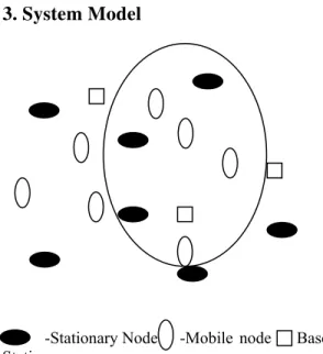
3. System Model
-Stationary Node -Mobile node Base Station
In real world, at a given time, there may be stationary, mobile and powerful base stations existing together in a region. Assuming all the nodes know their destination ID, when an event occurs or when requested by the base station, they try to forward the data to their base station. The topology changes continuously due to the mobility of the nodes. It will be practically impossible most of the times to directly forward the data to the base station due to the nature of radio signals. Hence the problem is to find a neighbour (hop) towards the destination. This is done repeatedly till the destination is reached. In a heterogeneous setup there may be a few base stations in a region. So we argue that for a given node to forward the data, it is enough to find the nearest base station even if the node’s base station is different. Also only high energy nodes get selected as relay nodes sparing the less energy stationary nodes thus prolonging the network life time.
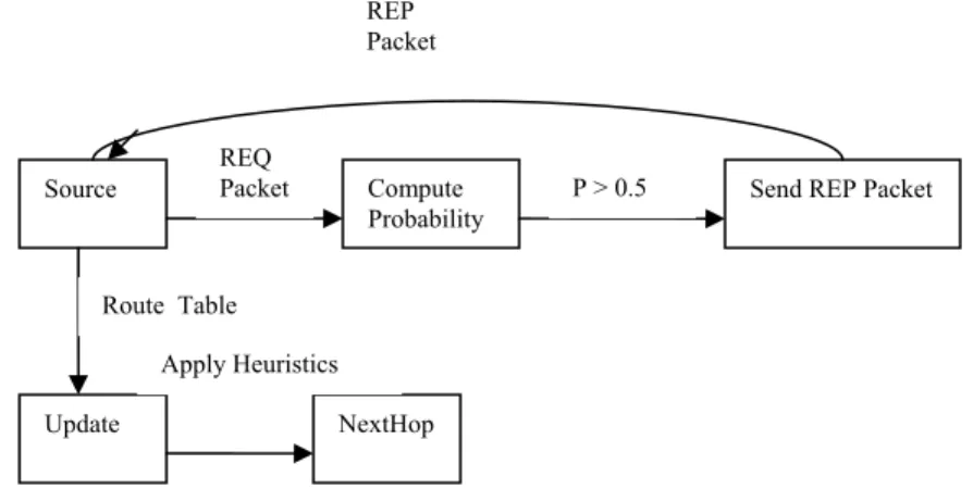
When a node senses an event, it sends a request packet which contains the Node ID, Destination ID , Time and Location. A node (i) which receives the request packet computes the probability of a link between itself and the source. The factors that are taken into consideration are the distance between the source and the node, the energy level of the node, the type of the node and the type of the node’s neighbours. The initial probabilities are set based on the type of the node. If the type is a base station or a sink node (Value : 2) , the probability p(i) is set to 0.75. If the type is a high energy rechargeable node (Value : 1) , the probability p(i) is set to 0.5 and for the low energy static node (Value : 0), p(i) is set to 0.1. The probability may be increased or decreased after receiving a request packet. If the probability is greater than 0.5, a reply packet is sent to the source node. Otherwise the request packet will be discarded. The reply packet consists of Neighbour ID, Location, Type, Time and the Probability. When a node receives a reply packet, it updates its routing table with Neighbour ID, Location, Time, Type and the Probability. Finally the node picks the best neighbour from the routing table by applying the A* search algorithm. All the nodes maintain a table of recent request/reply packets. When a request packet arrives, the node checks whether any recent reply packet had been sent to any node in the region, not necessarily to the source node. This is because of the fact that when an event occurs, all the nodes in the region (within a
specified radius) sense the same. After ‘t’ seconds the recent packets automatically get deleted from the table. This policy helps to avoid congestion and redundancy and is highly energy efficient.
Table 1: REQ Packet
Node ID Dest ID Location Time
Table 2: REP Packet
Node ID
Dest ID
Prob Type Location Seq no
Time
Table 3: Route Table Fields
Node ID
Neighbour ID
Prob Type Location Seq No
Time
3.1 A* Algorithm to find the best neighbour
The problem is to find a minimum cost path from a source to a destination. The optimum path in wireless sensor networks is the minimum energy conservation path. The algorithm works based on the type of node. Assuming high energy base stations and high bandwidth mobile nodes which could be recharged, the probabilities are set. The probability differs for each request. The static nodes with less energy level will not participate in routing in order to save energy. A* algorithm is applied to pick the best neighbour from the routing table of a node. The cost function is the distance between the source and the destination. Assuming intermediate base stations or sink nodes that will have the capacity to directly route the packet to the destination, we reduce the problem to finding the nearest base station problem. The heuristic function computes the link quality by combining the probability, type, time and the direction of the destination. As probabilities are self computed, when a reply packet arrives, the node instead of picking the highest probability node as the nextHop , checks the time stamp and the type. If there is a node with slightly less probability which arrived lately, the node will prefer it as a hop to forward the data rather than the high probability one. This is because of the mobility of the nodes.
C(i) = dist(i,j) , the distance between the source and the destination.
Fig. 2 Schematic Representation of the Model
If we form the convex hull of the nodes within a neighbourhood say a radius r, then only one node would be allowed to transmit at a given time. This avoids traffic congestion and redundancy.
Algorithm
1. Source Sends REQ packet
2. Node Receives REQ packet
3. Node Checks Recent REQ/REP List
4. If (! Recent)
a. Node Self computes
Probability P
b. If P >= 0.5 , node sends a REP packet
c. Else discard it; Exit; 5. Else Discard it; Exit;
6. Source receives a REP packet
7. Source updates the Route Table
8. Apply A* Algorithm to pick the best
neighbour
9. Forward Data to the next Hop
10. If the next Hop is the Destination , Exit; 11. Else If the next Hop is a base station ,
Exit;
12. Else Forward; Go to 1;
13. Return;
4. Mathematical Model
Let there be n number of nodes within a radius r. The problem is to find an optimal path from a source to a destination. Random Geometric Graphs (RGG) have been a very influential and well-studied model of large networks, such as sensor networks, where the network agents are represented by the vertices of the RGG, and the
direct connectivity between agents is represented by the edges. Informally, given a radius r, a random geometric graph results from placing a set of n vertices uniformly and independently at random on the unit torus [0, 1]2 and connecting two vertices if and only if their distance is at most r, where the distance depends on the chosen metric.
Connecting two vertices, u, v is possible if and only if the distance between them is at most a threshold r, ie. d (i, j) ≤ r. Several probabilistic results are known about the number of components in the graph as a function of the threshold r and the number of vertices n. An edge appears iff d(i,j) is less than r and if the probability computed based on the distance between i and j , type of j , neighbours of j and energy level of j is greater than a threshold value(0.5).
Let R(i,j) be the directed random geometric graph for the sensor model under study.
Then,
R(i,j) = 1 if p(i,j) > =0.5 = 0 , Otherwise
where p(i,j) = f(d(i,j) , e(j), t(j),n(j)) d(i,j) – Distance between i and j
e(j) – Remaining energy level of j = Ej – ek , k = 0 to j-1
t(j) = 0 for Low energy Static node 1 for High Energy Node 2 for Base station/ Sink node n(j) = 1 if the neighbour is a base station or the neighbour is close to a base station
Source Compute
Probability
Send REP Packet REQ
Packet P > 0.5
REP Packet
Update
Route Table
Fig. 3 RGG with selected path
We will denote s(i) as the set of all nodes in φ(i) whose distance to node N is smaller than predefined radius r. Decisions at node i will be based on the following variables:
1. An estimation of the available energy at
neighboring nodes, {Eij, j s(i)}.
2. The distance to each of the
neighbouring node , { min d(i,j) < r }
3. The neighbours type and closeness to a
base station , { t(j) = 2 or 1 , n(j) where t(n(j)) = 2 }
The following operations are possible in the graph.
1. Adding an edge – When a node receives a reply packet with probability greater than 0.5, an edge will be added.
2. Deleting an edge – Since the nodes could be mobile, after a specific time period, the probability of an edge may go down. In this case the edge will be deleted.
Assuming that most energy consumption is caused by transmissions, the estimation
E(i,j)k+1 = E(i,j) k – m(j) k ET(1)
where m(j) is the number of messages transmitted by node j at time k and ET is the energy consumed per transmission. Note that our model assumes that the energy consumptions are the same at each transmission (which is a
reasonable approximation if information is sent in packets of equal size), and that node i ’listens’ all transmissions done by its neighbor, j.
All these variables are grouped into observation vector x. Each node with a message to transmit states the decision as a result of solving a hypothesis testing problem with two hypotheses, T = 0 or T = 1, where:
• T = 1 if at least one neighbor will forward the message.
• T = 0 if no neighbor will forward the message in which case the message will be discarded. Depending on its belief about the value of T, node i will make decision D1 (the message is transmitted) or D0 (the message is not transmitted).
To do so, we define cost C(i,T) = 1 if j , p(i,j) > 0.5 = 0 , Otherwise
The optimal path can be obtained if all the nodes are reachable from a sink node or a base station in one or two hops. Otherwise the model is reduced to AODV. The topology can be reconstructed to prolong the network life time.
From the definition of the graph it follows that, this graph is not symmetric.
i.e, R(i,j) ≠ R(j,i)
Proof: Assume i is not in the proximity of a base station and j is closer to a base station. So j’s Base Station/
Sink Node Static Less Energy Node
computed probability is high and the link exists between i and j. On the contrary, the probability computed by i will be low either because of its type or due to the proximity of the node. So j will not select i as the next Hop to reach its destination. So there is no edge between j and i.
There may be isolated vertices in this model as nodes with less energy level are less likely to participate in routing. So the graph is not a connected graph. Only one edge within the radius is selected for transmission and so the order of the algorithm is O(1).
5. Performance Analysis
We simulate this protocol on GloMoSim, [26] a scalable discrete-event simulator developed by
UCLA. This software provides a high fidelity simulation for wireless communication with detailed propagation, radio and MAC layers. We compare the routing protocol named as HLAODV with two popular sensor networks routing protocols – AODV and DSR
5.1 Simulation Model
The GloMoSim library [26] is used for protocol development in sensor networks. The library is a scalable simulation environment for wireless network systems using the parallel discrete event simulation language PARSEC. The distributed coordination function (DCF) of IEEE 802.11 is used as the MAC layer in our experiments. It uses Request-To-Send (RTS) and Clear-To-Send (CTS) control packets to provide virtual carrier Table 4: Assumed Parameters
Parameters Value
Transmission range 250 m
Simulation Time 5M
Topology Size 2000m x 2000m
Number of sensors 55
Number of sinks 16
Mobility Trace File
Traffic type Constant bit rate
Packet rate 8 packets/s
Packet size 512 bytes
Radio Type Standard
Packet Reception SNR
Radio range 350m
MAC layer IEEE 802.11
Bandwidth 2Mb/s
Node Placement Node File
Initial energy in batteries 10 Joules
Signal Strength Threshold -80 dbm
Energy Threshold 0.001mJ
sensing for unicast data packets to overcome the well-known hidden terminal problem. There are some initial values used in the simulation. Table 4 lists the assumed parameters. Intel Research Berkeley Sensor Network Data and WiFi CMU data from Select Lab [28] are used to get the positions for the nodes. The experiment is repeated for varying number of nodes. CBR traffic is assumed in the model. For mobility, trace file is used. The new protocol is written in Parsec and hooked to GloMoSim. All the three protocols are simulated in GloMoSim to enable
comparisons among them. When a packet is generated, the corresponding routing algorithm is invoked.
5.2 Performance Metrics
Latency – This is a measure of execution time. It is the total time taken by the various protocols for the given CBR traffic to complete within the simulation time.
Energy Spent – This is measured in terms of
signals received and transmitted. The energy spent on each node is directly proportional to the number of signals received and transmitted. Less number is an indicative of energy conservation.
Congestion – The parameters for congestion
evaluation are number of collisions and number of timeout packets generated. Obviously more number of collisions and timeout packets indicate congestion in the traffic.
Load Balance - The number of nodes used in
the transmission. This is also an indication of energy conservation at each node.
5.3 Simulation Results
Figure 4 shows the execution time of three protocols for different sets of nodes and traffic. The execution time increases as the traffic increases. Due to control packets overhead in route discovery and maintenance AODV and DSR have high execution time as against the proposed protocol. Both AODV and DSR do not differentiate nodes. When there are no base stations HLAODV tends to take more time than AODV and DSR protocol.
Execution Time
0 1 2 3 4 5 6
1 2 3 4 5 6 7 8
CBR Traffic
Ti
m
e HLAODV
AODV DSR
Fig 4. Packet Delivery Time
Figures 5 and 6 show the number of signals received and transmitted by the nodes. There is equal energy spent on receiving phase as transmission phase. There is a sharp difference in signals received in the new protocol as compared to others. In signals transmitted there are only a
few nodes are affected in HLAODV. The graphs are indicative of less energy spent in HLAODV compared to AODV and DSR. This clearly indicates the energy efficiency of the HLAODV protocol.
Signals Received
0 5000 10000 15000 20000 25000 30000 35000 40000 45000
1 5 9 13 17 21 25 29 33 37 41 45 49 53
Node
Si
g
na
ls HLAODV
AODV DSR
Fig 5. Total Number of Signals Received
Signals Transmitted
0 200 400 600 800 1000 1200 1400 1600 1800 2000
1 5 9 13 17 21 25 29 33 37 41 45 49 53
Node
S
igna
ls HLAODV
AODV DSR
Fig 6. Total number of Signals Transmitted
Number of Collisions 0 200 400 600 800 1000 1200 1400 1600
1 5 9 13 17 21 25 29 33 37 41 45 49 53
Nodes C o lli s io n s HLAODV AODV DSR
Fig 7 . Number of Collisions
TimeOut Packets Generated
0 0.5 1 1.5 2 2.5 3 3.5 4 4.5 5 5.5 6
1 5 9 13 17 21 25 29 33 37 41 45 49 53
Hu nd re d s Node C TS Ti m e out P a c k e ts HLAODV AODV DSR
Fig 8. Time out Packets Generated
6. Conclusion
Wireless sensor networks and radio frequency identification (RFID) devices are quickly becoming a vital part of our infrastructure with applications ranging from supply-chain management to home automation and healthcare. These tiny, pervasive computing devices have extremely limited power resources and computational capabilities. On the other side there also exist heterogeneous wireless networks in which devices have dramatically different capabilities. In this paper we proposed an energy efficient routing protocol for heterogeneous pervasive networks based on location. Simulation results show that our protocol HLAODV outperforms AODV and DSR in energy efficiency, latency, load balancing, redundancy suppression and congestion control. The model is a cross layer design as the link parameters determine the routing scheme. Our next goal is to identify the minimum number of base stations required to get an optimal path and to study a secure routing scheme for heterogeneous networks.
7. References
[1]. Ahmed H. Zahran, Cormac J. Sreenan, “Threshold-Based Media Streaming Optimization for Heterogeneous Wireless Networks” , IEEE Transactions On Mobile Computing, Vol. 9, No. 6, 2010 ,753
[2]. A. H. Azni, Madihah Mohd Saudi, Azreen Azman, and Ariff Syah Johari D , “Performance Analysis of Routing Protocol for WSN Using Data Centric Approach” , World Academy of Science, Engineering and Technology , 2009 , 53 [3]. Bandyopadhyay S and Coyle E , “ An energy
efficient hierarchical clustering algorithm for wireless sensor networks” , IEEE Infocom , 2003, pp 1713-23
[4]. Bharat Kumar Addagada, Vineeth Kisara and Kiran Desai , “A Survey: Routing Metrics for Wireless Mesh Networks” , 2009
[5]. Bhardwaj M, Garnett T and Chandrakasan A P , “ Upper bounds on lifetime of sensor networks”, IEEE International Conference on Communications (Helsinki) , 2001, pp 785-790 [6]. Bhupendra Gupta , Srikanth K Iyer , D
Manjunath , “Topological Properties Of The One Dimensional Exponential Random Geometric Graph”, Random Structures & Algorithms , Volume 32 , Issue 2 , 2008, pp: 181-204
[7]. Chen Avin , “Random Geometric Graphs: An Algorithmic Perspective” , Ph,D dissertation, University of California , Los Angeles , 2006 [8]. L. Chen, S. H. Low, M. Chiang, J. C. Doyle ,
“Cross-Layer Congestion Control, Routing and Scheduling Design in Ad Hoc Wireless Networks”, IEEE International Conference on Computer Communications. Proceedings In INFOCOM , 2006, pp. 1-13.
[9]. T. Clausen, Ed., P. Jacquet, “ Optimized Link State Routing Protocol (OLSR)” , Network Working Group, Request for Comments: 3626 [10].S. Das, R. Castaneda, and J. Yan, ,
"Simulation-Based Performance Evaluation of Routing Protocols for Mobile Ad Hoc Networks", Mobile Networks and Applications, Vol. 5, No. 3, 2000, pp 179-189
[11].J. D´ıaz D. Mitsche X. P´erez-Gim´enez , “On the Connectivity of Dynamic Random Geometric Graphs, Symposium on Discrete Algorithms” , Proceedings of the nineteenth annual ACM-SIAM symposium on Discrete algorithms , 2008, pp 601-610
[12].Feilong TANG, Minyi GUO, Minglu LI, Cho-Li WANG , Mianxiong Dong, “Secure Routing for Wireless Mesh Sensor Networks in Pervasive Environments”, International Journal Of Intelligent Control And Systems , VOL. 12, NO. 4, 2007, pp 293-306
in Proc. of ACM MobiCom’00, Boston, MA, USA, 2000, pp. 56–67
[14].Jamal N. Al-Karaki Ahmed E. Kamal , “Routing Techniques in Wireless Sensor Networks: A Survey” , 2004
[15].D. B. Johnson, D. A. Maltz, and Y-C Hu., “ The Dynamic Source Routing Protocol for Mobile Ad Hoc Networks (DSR)” , IETF Mobile Ad Hoc Networks Working Group, Internet Draft , 2003 [16].Karp, B.; Kung, H. T. , “GPSR: Greedy
perimeter stateless routing for wireless networks”, In Proceedings of the Sixth Annual ACM/IEEE International Conference on Mobile Computing and Networking (MobiCom), Boston, USA, 2000, pp. 243–254.
[17].Ko, Y. B.; Vaidya, N. H. , “Location-Aided Routing (LAR) in mobile ad hoc networks”, Wireless Networks , 6, 2000, 307–321
[18].F. L. LEWIS , “Wireless Sensor Networks - Smart Environments: Technologies, Protocols, and Applications” , ed. D.J. Cook and S.K. Das, John Wiley , 2004
[19].Na Wang and Chorng Hwa Chang , “Performance analysis of probabilistic multi-path geographic routing in wireless sensor networks” , International Journal of Communication Networks and Distributed Systems , Vol 2 , 2009, pp 16 – 39
[20].Ning Li , Jennifer C. Hou , “Topology Control in Heterogeneous Wireless Networks: Problems and Solutions”, IEEE/ACM Transactions on Networking (TON) , Volume 13 , Issue 6 , 2005, pp 1313 - 1324
[21].C. E. Perkins, E. M. Royer, and S. R. Das, “Ad Hoc On-Demand Distance Vector (AODV) Routing” , IETF Mobile Ad Hoc Networks Working Group, IETF RFC 3561
[22].C. E. Perkins and P. Bhagwat, , “Highly dynamic destination-sequenced distance-vector routing (DSDV) for mobile computers” . In Proceedings of the ACM Special Interest Group on Data Communications (SIGCOMM), 1994, pp 234-244
[23].J. Polastre, R. Szewcyk, A. Mainwaring, D. Culler, J. Anderson, “Analysis of Wireless Sensor Networks for Habitat Monitoring in Wireless Sensor Networks” , Kluwer Academic Publishers (NY), 2004, pp. 399-423.
[24].Robert Grimm, Tom Anderson, Brian Bershad, and David Wetherall , “A System Architecture for Pervasive Computing”, ACM SIGOPS European Workshop, Proceedings of the 9th workshop on ACM SIGOPS European workshop: beyond the PC: new challenges for the operating system , 2000, pp 177 - 182
[25].M. Singh and V.K. Prasanna, “Optimal energy-balanced algorithm for selection in a single-hop sensor network”, IEEE international workshop on SNPA ICC, 2003
[26].M. Takai, L. Bajaj, R, Ahuja, R. Bagrodia and M. Gerla, “GloMoSim: A Scalable Network
Simulation Environment”, Technical report 990027, UCLA , 1999
[27].Uichin Lee, Eugenio Magistretti, Biao Zhou, Mario Gerla, Paolo Bellavista, Antonio Corradi, “Efficient Data Harvesting in Mobile Sensor Platforms” , percomw, 2006, pp.352-356, Fourth IEEE International Conference on Pervasive Computing and Communications Workshops (PERCOMW'06)
[28].Wireless Sensors Location Data :
http://www.select.cs.cmu.edu/data/index.html [29].Xiang-Yang Li , Wen-Zhan Song , Yu Wang ,
“Localized topology control for heterogeneous wireless sensor networks” , ACM Transactions on Sensor Networks (TOSN) , Volume 2 , Issue 1 , 2006, pp 129 - 153
[30].YAO Kung , “Sensor Networking: Concepts, Applications, and Challenges”, ACTA Automatica Sinica , Vol. 32, No. 6 , 2006
[31].Ye, F.; Zhong, G.; Lu, S.; Zhang, L. , “GRAdient broadcast: a robust data delivery protocol for large scale sensor networks” , Wireless Networks, 11(3), 2005 , pp 285-298. [32].Zhang Jin , Yu Jian-Ping , Zhou Si-Wang , Lin