Performance and results of the high-resolution biogeochemical model PELAGOS025 within NEMO

(1)

GMDD

8, 10585–10625, 2015

Performance of PEALGOS025 model

I. Epicoco et al.

Title Page

Abstract Introduction

Conclusions References

Tables Figures

◭ ◮

Back Close

Full Screen / Esc

Printer-friendly Version Interactive Discussion

Discussion

P

a

per

|

Discussion

P

a

per

|

Discussion

P

a

per

|

Discussion

P

a

per

|

Geosci. Model Dev. Discuss., 8, 10585–10625, 2015 www.geosci-model-dev-discuss.net/8/10585/2015/ doi:10.5194/gmdd-8-10585-2015

This discussion paper is/has been under review for the journal Geoscientific Model Development (GMD). Please refer to the corresponding final paper in GMD if available.

Performance and results of the

high-resolution biogeochemical model

PELAGOS025 within NEMO

I. Epicoco1,2, S. Mocavero2, F. Macchia2, M. Vichi3, T. Lovato2, S. Masina2, and G. Aloisio1,2

1

Department of Innovation Engineering, University of Salento, via per Monteroni, 73100 Lecce, Italy

2

Euro-Mediterranean Centre on Climate Change, via Augusto Imperatore 16, 73100 Lecce, Italy

3

Department of Oceanography, University of Cape Town, Cape Town, South Africa

Received: 3 November 2015 – Accepted: 26 November 2015 – Published: 16 December 2015

Correspondence to: I. Epicoco ([email protected])

(2)

GMDD

8, 10585–10625, 2015

I. Epicoco et al.

Title Page

Tables Figures

◭ ◮

Back Close

Full Screen / Esc

Discussion

P

a

per

|

Discussion

P

a

per

|

Discussion

P

a

per

|

Discussion

P

a

per

|

Abstract

The present work aims at evaluating the scalability performance of a high-resolution global ocean biogeochemistry model (PELAGOS025) on massive parallel architec-tures and the benefits in terms of the time-to-solution reduction. PELAGOS025 is an on-line coupling between the physical ocean model NEMO and the BFM

biogeochem-5

ical model. Both the models use a parallel domain decomposition along the horizontal dimension. The parallelisation is based on the message passing paradigm. The per-formance analysis has been done on two parallel architectures, an IBM BlueGene/Q at ALCF (Argonne Leadership Computing Facilities) and an IBM iDataPlex with Sandy Bridge processors at CMCC (Euro Mediterranean Center on Climate Change). The

10

outcome of the analysis demonstrated that the lack of scalability is due to several fac-tors such as the I/O operations, the memory contention, the load unbalancing due to the memory structure of the BFM component and, for the BlueGene/Q, the absence of a hybrid parallelisation approach.

1 Introduction

15

Nowadays, the study of climate change needs high-resolution simulations as one of the possible strategies to reduce uncertainty in climate predictions. In addition, the in-teraction of the physical components of the climate system with Earth biogeochemistry and socio-economical aspects implies that multiple dynamical models are coupled to-gether in the so-called Earth System Models (Schellnhuber, 1999; Claussen, 2000),

20

increasing the complexity of the software tool. Next-generation leadership class com-puting systems can be considered as a deep revolution on climate change applications (Dongarra et al., 2011), allowing ever higher resolutions of climate models that will match or even surpass the resolution of today’s operational weather forecast models. In particular, exascale will be able to provide the computational resources needed to

25

(3)

GMDD

8, 10585–10625, 2015

I. Epicoco et al.

Title Page

Tables Figures

◭ ◮

Back Close

Full Screen / Esc

Discussion

P

a

per

|

Discussion

P

a

per

|

Discussion

P

a

per

|

Discussion

P

a

per

|

and Earth System simulations can benefit from exascale as long as the models are capable to scale their performances. There are several issues to be considered when scaling models to reach performance up to an order of 1018 floating point operations per second (Washington, 2008). At higher resolution, new physical aspects must be taken into account and integrated into the climate models (see, e.g., Siedler et al.,

5

2013); it is necessary to design scalable computational kernels and algorithms, as well as considering new approaches and paradigms in the parallel programming in order to follow the features of the exaflops architectures. Often, to exploit the exascale poten-tiality, the so-called “legacy” climate models require a deep re-engineering, like e.g., the improvement of the computational kernels, new parallel approaches and new scalable

10

algorithms. Moreover, new models, dynamic grids and new numerical solvers have to be conceived on exascale computers to carry out efficient operations.

The community climate models have to be carefully analysed in order to empha-sise the scalability bottlenecks, which could not be the same on di_fferent architectures. Moreover, the implemented parallel approaches and the available alternatives have to

15

be investigated to select the best strategy. The computational scientists have to decide if the model has to be re-designed from scratch or if it can be optimised in order to exploit the new generation architectures. The performance could be improved by us-ing optimised numerical libraries (Dongarra et al., 1988, 1990; Blackford et al., 1996; Balay et al., 1997) or using tools to improve the I/O operations (XIOS, 2012; Balaji

20

et al., 2013). In any case, the first required step is the analysis of the model scalability on (as many as possible) multiple architectures for testing the behaviour on heteroge-neous resources. Dennis and Loft (2011) stressed the importance of testing the weak scalability by studying the impact of increasing both the resolution and core counts by factors of 10 to 100 using the Community Climate System Model (CCSM). Several

25

(4)

GMDD

8, 10585–10625, 2015

I. Epicoco et al.

Title Page

Tables Figures

◭ ◮

Back Close

Full Screen / Esc

Discussion

P

a

per

|

Discussion

P

a

per

|

Discussion

P

a

per

|

Discussion

P

a

per

|

and the IBM BG/P for four representative production simulations, by varying both the problem size and the included physical processes. The bottleneck can be a particu-lar kernel of the model or a particuparticu-lar operation, such as the I/O, or an entire model component within a coupled model, which is likely to be rather common with coupled Earth System Models. The scalability of a coupled model can be improved balancing

5

the model components load (Epicoco et al., 2011) or optimising the component that limits the performance. Mirin and Worley (2012) identified the CESM atmosphere com-ponent (CAM) as the most computationally expensive. The improvement of the CAM performance scalability can be achieved by means of new optimised communication protocols, and through the reduction of the computational bottlenecks.

10

As an example of this assessment of multi-component Earth System Models, we focused on an implementation that is likely to be standard in the next generation of climate models. We considered two components that are usually computationally de-manding, the ocean physics and ocean biogeochemistry. As in most of the cases, ocean biogeochemical models are tightly linked to the ocean physics computational

15

cores, as they share the same grid and numerical schemes. In particular, the present work aims at analysing the computational performance of the Nucleus for the European Modelling of the Ocean (NEMO) oceanic model at 0.25◦ of horizontal resolution cou-pled with the Biogeochemical Flux Model (BFM). The paper is organised as follows: the next section introduces the coupled model and the experimental set-up, Sect. 3

20

shows the main results in terms of strong scalability of the model, Sect. 4 describes the methodology used for the code profiling focusing on two different architectures, Sect. 5 discusses about the data structures used in NEMO and in BFM and highlights pros and cons, Sect. 6 illustrates the memory allocation model and the last section ends with some conclusions and future perspectives.

(5)

GMDD

8, 10585–10625, 2015

I. Epicoco et al.

Title Page

Tables Figures

◭ ◮

Back Close

Full Screen / Esc

Discussion

P

a

per

|

Discussion

P

a

per

|

Discussion

P

a

per

|

Discussion

P

a

per

|

2 The PELAGOS025 biogeochemical model

PELAGOS (PELAgic biogeochemistry for Global Ocean Simulations, Vichi et al., 2007; Vichi and Masina, 2009) is a coupling between the NEMO general circulation model (version 3.4, http://www.nemo-ocean.eu) and the Biogeochemical Flux Model (BFM, version 5, http://bfm-community.eu). The BFM model is based on a biomass

contin-5

uum description of the lower trophic levels of the marine system. The model is meant to describe the planktonic ecosystem in the global ocean, therefore it complements the classical ocean carbon cycle equations with the fluxes of nutrients (nitrogen, phospho-rus, silicate and iron) among multiple biological functional groups, namely phytoplank-ton, zooplankton and bacteria. From a computational point of view, the use of multiple

10

chemical constituents to represent the functional groups implies the implementation of several state variables that is about 2 to 3 times larger than the standard carbon cy-cle models (this current formulation has 52 state variables, see Vichi et al., 2015a for a description of the equations). In addition, the model is capable to store all the rates of transfer of the constituents among the functional groups, which adds substantially to

15

the computational load.

The coupling between NEMO and the BFM is fully detailed in Vichi et al. (2015b), available in the BFM web site. The BFM is zero-dimensional by construction and de-fined only in the ocean points of the model grid. This implies that each BFM variable is a one-dimensional array, with all the land points stripped out from the three-dimensional

20

domain of NEMO and the remapping into the ocean grid is done only when dealing with transport processes. This operation is done for every subdomain of the grid decompo-sition.

NEMO uses a horizontal domain decomposition based on a pure MPI approach. Once the number of cores has been chosen, the number of subdomains along the

25

(6)

GMDD

8, 10585–10625, 2015

I. Epicoco et al.

Title Page

Tables Figures

◭ ◮

Back Close

Full Screen / Esc

Discussion

P

a

per

|

Discussion

P

a

per

|

Discussion

P

a

per

|

Discussion

P

a

per

|

cross stencil. The best decomposition strategy for reducing the communication over-head is to select jpni and jpnj to obtain subdomains as much square as possible. By following this procedure, the communication overhead is minimum. However, coupling the biogeochemical component, the number of the ocean points for each subdomain becomes a crucial factor, since BFM, unlike NEMO, performs the computation only on

5

these points. A pre-processing tool has been written to establish the best domain de-composition that minimises the number of ocean points of the biggest subdomain. In addition, a NEMO feature allows to exclude the domains with only land points. Reid (2009) demonstrated that the removal of land processes reduces the resource usage by up to 25 % and also gives a small reduction in the total runtime. The subdomains

10

to be excluded depend on the bathymetry. Figure 1 shows a domain decomposition with the bathymetry in background highlighting those subdomains excluded from the computation because made of only land points.

3 Performance analysis

3.1 Test case

15

The PELAGOS model was tested in this work at the highest available horizontal reso-lution of 0.25◦

described in McKiver et al. (2015), where all the details of the simulation set-up can be found. PELAGOS025 is a configuration based on the ORCA025 grid (1442×1021 grid points in the horizontal with 50 vertical levels), going from an

ef-fective resolution of 28 km at the Equator to 10 km at the Poles (Barnier et al., 2006).

20

A time step of 18 min is used both for the physical and biogeochemical model, while the sea ice model is called every 5 steps. For each run we simulated one day with a total of 80 time steps. This specific experiment focused more on computational performances and less on the I/O behaviour because, at the time of the experimental analysis, it was possible to use a I/O strategy where each process wrote its own outputs and restarts

25

(7)

GMDD

8, 10585–10625, 2015

I. Epicoco et al.

Title Page

Tables Figures

◭ ◮

Back Close

Full Screen / Esc

Discussion

P

a

per

|

Discussion

P

a

per

|

Discussion

P

a

per

|

Discussion

P

a

per

|

efficiently handled by the filesystem. Further experiments will be performed using the XIOS (XIOS, 2012) library that will be supported from version 3.6 of NEMO.

The analysis of the strong scalability of the code has been performed on two ar-chitectures: the first one is a BlueGene/Q (named VESTA), located at the Argonne Leadership Computing Facilities (ALCF/ANL); the second one is the ATHENA system,

5

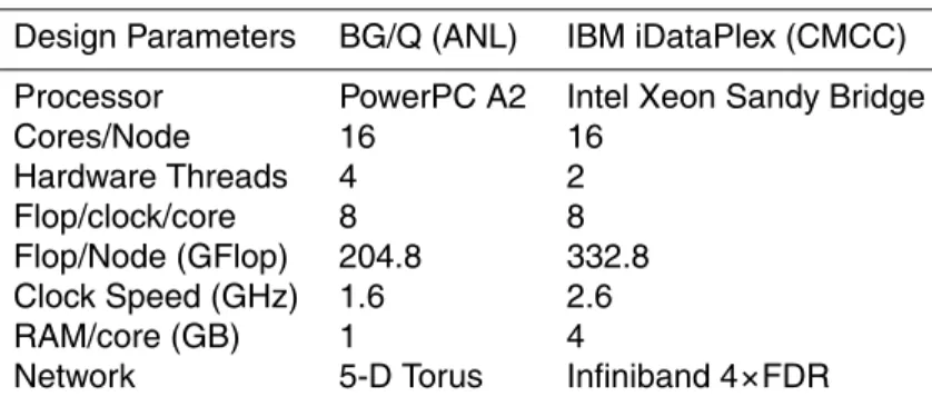
available at CMCC, an iDataPlex equipped with Intel Sandy Bridge processors. The activity has been conducted in collaboration with the ALCF/ANL. Details about the systems are reported in Table 1. The main differences among the machines are the number of hardware threads. VESTA can handle Simultaneous Multi Threading (SMT) up to 4 threads while the Sandy Bridge architecture supports the execution of 2 threads

10

simultaneously. Even if ATHENA has a higher value of the peak performance per node, VESTA is a very high scalable architecture. Finally the communication network is dif-ferent, BG/Q uses a Torus network with 5 dimensions, it is characterised by several partitions made of 32 up to 1024 nodes. During the execution, an entire partition is reserved to the job. This means that the job acquires the use of both the nodes and the

15

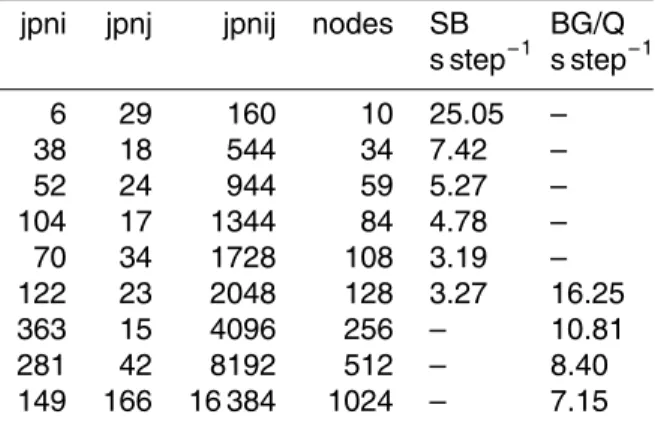
network partition exclusively. The ATHENA nodes are connected through an infiniband switch that is shared among all the running jobs. Table 2 reports the considered do-main decomposition corresponding to the selected number of cores on ATHENA and VESTA machines. The table also contain the number of nodes used for each experi-ment. SMT has not been used on both the machines. Being NEMO a memory-intensive

20

application, the use of SMT does not produce major improvements in the performance; noteworthy, performance can even deteriorate due to the memory contention produced by the simultaneous execution of the threads. Each experiment has been repeated 5 times with 30 total runs on ATHENA and 20 on VESTA.

3.2 Strong scalability

25

(8)

num-GMDD

8, 10585–10625, 2015

I. Epicoco et al.

Title Page

Tables Figures

◭ ◮

Back Close

Full Screen / Esc

Discussion

P

a

per

|

Discussion

P

a

per

|

Discussion

P

a

per

|

Discussion

P

a

per

|

ber of computing elements increases for a fixed problem size; the latter describes how the execution time changes with the number of computing elements for a fixed grain size. This means that the computational work assigned to each processor is fixed and hence the problem size grows with the number of processes. The weak scalability is relevant when a parallel architecture is used for solving problems with a variable size

5

and the main goal is to improve the solution accuracy rather than to reduce the time-to-solution. The strong scalability is relevant for applications with a fixed problem size and hence the parallel architecture is used to reduce the time-to-solution. The PELA-GOS025 coupled model can be considered as a problem with a fixed size and the main goal is to use computational power to reduce the time-to-solution.

10

The charts in Figs. 2, 3 and 4 show the scalability results respectively in terms of speedup, execution time and SYPD (Simulated Years Per Day), a metric for measur-ing the simulation throughput usually referred by the climate scientists to evaluate the model performance (see, e.g., Parashar et al., 2010). For both machines the results show that the MPI communication time tend to decrease with the number of cores

15

for two main reasons. The first one relates to the communication type that can be classified as neighbourhood collective, where each process communicates only with its neighbours and no global communication happens; this means that the number of messages per core does not change when the number of processes increases. The second reason involves the amount of data exchanged between processes that

be-20

comes smaller when the local subdomain shrinks. On the ATHENA cluster, the tests have been executed up to 2048 cores. Figure 3 shows that the execution time on 2048 cores increases with respect to the run on 1728 cores, which indicates a lack of scal-ability. For this reason the analysis on ATHENA was limited to 2048 cores. On VESTA machine the analysis has been performed up to 16 384 cores. Even if there is a

fac-25

(9)

GMDD

8, 10585–10625, 2015

I. Epicoco et al.

Title Page

Tables Figures

◭ ◮

Back Close

Full Screen / Esc

Discussion

P

a

per

|

Discussion

P

a

per

|

Discussion

P

a

per

|

Discussion

P

a

per

|

4 Code profiling

The optimisation process of a code requires the analysis of the bottlenecks that limit the scalability. The investigation methodology used in the present work is based on the analysis at the routine level. Two di_fferent reference decompositions have been taken into account and the execution time of the main routines for the two decompositions

5

have been analysed in order to evaluate the speed-up of each single routine. The gprof utility as been used for measuring the execution time of the PELAGOS routines. The gprof output consists of two parts: the flat profile and the call graph. The flat profile gives the total execution time spent in each function and its percentage of the total running time providing an easy way to identify the hot spots. Only the routines with

10

a percentage of the total running time greater than 1 % have been reported in the analysis.

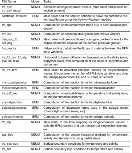
In addition, on the BG/Q machine, an in-depth analysis using the High Performance Monitor (HPM, Lakner et al., 2008) tool has been performed in order to verify the overall intrinsic performance. For reference, a complete description of the code flow chart and

15

naming conventions of the various routines is available in the BFM manuals (Vichi et al., 2015a, b). We report in Table 3 a description of the main tasks performed by the routines that have been identified by the code profiling on the two architectures.

4.1 BG/Q

The profiling at routine level helps to discover the model bottlenecks. The code

profil-20

ing has been performed with 2048 and 4096 cores. The most time consuming routines have been selected in both cases. Figure 5 shows the speedup for the main identified routines. The speedup is evaluated as ratio between the execution time on 2048 and 4096 cores, so the ideal value should be 2. However, none of the routines reached the ideal speedup. This is because the computing time for the BFM model strictly depends

25

(10)

pro-GMDD

8, 10585–10625, 2015

I. Epicoco et al.

Title Page

Tables Figures

◭ ◮

Back Close

Full Screen / Esc

Discussion

P

a

per

|

Discussion

P

a

per

|

Discussion

P

a

per

|

Discussion

P

a

per

|

cess is respectively 28 553 and 19 506. Even if the number of cores has been doubled, the maximum number of ocean points has not been halved. The scalability of BFM is thus heavily affected by the load balancing problem. Moreover, the three routines, highlighted in Fig. 5 (cf. Table 3), are unaffected by scaling.

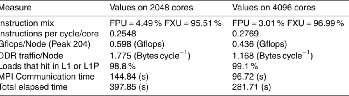
Table 4 shows the results got by applying the HPM on the BG/Q machine. The

in-5

struction mix refers to the ratio between the floating point and the total instructions. The best mix should be 50 %. BG/Q has 2 different and independent pipelines for executing floating point and integer instructions: an instruction on the Floating Point Unit (FPU) can be executed simultaneously with an instruction on the Fixed Point Unit (FXU). The instruction mix is completely unbalanced. However, we have to consider that the FXU

10

includes the load and store instructions to access the memory. Moreover, the execution reaches a rate of 2.7 Gflops per node which is only 0.25 % of the peak performance. This means that NEMO exploits only a very small part of the computational potentiality of the architecture. The main reason has to be found in the parallelisation approach based on pure MPI. The SMT is not exploited at all executing only one thread per core.

15

A hybrid parallel approach could better exploit the SMT improving the performance of the entire model. Last consideration regards the percentage of L1 cache hits: the high value means that the memory hierarchy is well exploited.

4.2 IBM iDataPlex

The analysis of routines scalability on the iDataPlex architecture has been performed

20

on two other reference decompositions respectively on 1344 and 2048 cores. Figure 6 shows the results in terms of speedup. In this case, the number of ocean points of the most loaded process is respectively 46 693 and 30 863, so that the ratio between both the number of ocean points and between the number of cores is about 1.5. The ocean points balancing among the subdomains is random and happens only for the

25

(11)

GMDD

8, 10585–10625, 2015

I. Epicoco et al.

Title Page

Tables Figures

◭ ◮

Back Close

Full Screen / Esc

Discussion

P

a

per

|

Discussion

P

a

per

|

Discussion

P

a

per

|

Discussion

P

a

per

|

The two considered architectures deeply differ in terms of processor technology, func-tional units, computafunc-tional datapath, memory hierarchy, network interconnection and software stack such as compilers and libraries. The BG/Q is based on light-weight processors at 1.6 GHz mainly suited for that part of the code which are computing in-tensive with massive use of floating point operations and with a high level of arithmetic

5

intensity. Moreover the optimisations introduced by the compiler are mainly related to the vectorisation level and this can explain why the routine identified on IBM-iDataPlex with Sandy Bridge processor are different from those ones identified on BG/Q. Further analyses are needed in order to discover the peculiarities of the highlighted routines or the presence of common issues, such as a high communication overhead or a low

10

parallelism level. In this case the performance could be improved introducing a hybrid parallelisation approach.

5 NEMO and BFM data structures

In this section we deeply analyse the differences between the data structures adopted in NEMO and in BFM and we evaluate which one is better to be used. A

three-15

dimensional matrices data structure is used in NEMO. Each matrix includes also the points over land and it is the natural implementation of the subdomains defined as regular meshes by the finite difference numerical scheme. Even if this data structure brings some overhead due to the computation and memorisation of the points over land, it maintains the topology required by the numerical domain. The finite difference

20

scheme requires each point to be updated considering its six neighbours, establishing a topological relationship among each point in the domain. Using a three-dimensional matrix to implement the numerical scheme, this relationship is maintained and the topo-logical position of a point in the domain can be directly derived by its three indexes in the matrix. Changing this data structure would imply the adoption of additional

infor-25

(12)

GMDD

8, 10585–10625, 2015

I. Epicoco et al.

Title Page

Tables Figures

◭ ◮

Back Close

Full Screen / Esc

Discussion

P

a

per

|

Discussion

P

a

per

|

Discussion

P

a

per

|

Discussion

P

a

per

|

to indirect memory references, introduction of cache misses and reduction of the loop vectorisation level.

The BFM model uses instead a one-dimensional array data structure with all the land points striped out from the three-dimensional domain. The BFM model is zero-dimensional by construction, so the new value of a state variable in a point depends

5

only on the other state variables in the same point and no relationship among the points is needed. The transport term of the pelagic variables is demanded to NEMO and this requires a remapping from one-dimensional to three-dimensional data struc-ture and viceversa at each coupling step. In this section we aim at evaluating if the adoption of the three-dimensional matrices data structure for BFM can improve the

10

performance of the whole model. Three main aspect will be evaluated: the number of floating point operations, the load balancing and the main memory allocation. The evaluation has been conducted by choosing a number of processes that lead each subdomain of PELAGOS025 configuration to have exactly a square shape. Figure 7 depicts all of the parallel decompositions that satisfy this squared domain condition.

15

A pair of number of processes along i and j which fall in the blu region generates a squared domain decomposition. The graph has been generated considering that in order to obtain a squared domain with just one line for the halo, the following equation must be satisfied:

_iglo-3

px

=

_jglo-3

py

py, px∈N 20

where iglo and jglo are the size of the whole domain and px and py are the number of processes to choose. With this choice any effect due to the shape of the domain is eliminated. In the following sub sections we analyse the three performance aspects keeping in mind that the aim is to compare the BFM model when it adopts one- or three-dimensional data structure. The analysis is not to be intended as a comparison

25

(13)

GMDD

8, 10585–10625, 2015

I. Epicoco et al.

Title Page

Tables Figures

◭ ◮

Back Close

Full Screen / Esc

Discussion

P

a

per

|

Discussion

P

a

per

|

Discussion

P

a

per

|

Discussion

P

a

per

|

5.1 Number of floating point operations

The number of floating point operations is directly proportional to the number of points included in the subdomain. Since a parallel application is driven by the most loaded process in the pool, we will evaluate how the number of points changes at di_fferent de-compositions for the process with the biggest domain considering the two data

struc-5

tures. Figure 8 reports the ratio between the number of points of the biggest domain for the three-dimensional (hence including the land points) and the one-dimensional data structure. For small decompositions (less than 1026) the three-dimensional data struc-ture includes an overhead due to the operations over the land points which reaches 12 %. When the number of processes increases, even if the subdomains become

10

smaller and the most loaded process should include only ocean points, the three-dimensional approach introduces a 2 % of computational overhead since the last level in the bottom is composed entirely by land points.

5.2 Load balancing

The load balancing is measured evaluating how many points are taken by each

pro-15

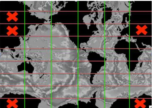
cess. An optimal load balancing is reached when each process elaborates the same number of points. With the three-dimensional data structure the global domain is equally partitioned among the processes; in the case that the domain size is not per-fectly divisible by the number of processes (along i or j direction), some processes have one additional row or column. In this case the work load is well balanced. Figure 9

20

graphically represents the amount of points for each domain. Each square is a process and the color represents the number of points (the lighter is the color, the lower is the number of points). The black squares are those domains made entirely by land points and they are excluded from the computation. With the one-dimensional data structure the work load balancing is different, as illustrated in Fig. 9. In this case the number

25

(14)

GMDD

8, 10585–10625, 2015

I. Epicoco et al.

Title Page

Tables Figures

◭ ◮

Back Close

Full Screen / Esc

Discussion

P

a

per

|

Discussion

P

a

per

|

Discussion

P

a

per

|

Discussion

P

a

per

|

and an estimation of how much improvement can be reached with an ideal distribution of the ocean points among the processes. The overhead due to the load balancing ranges from 50 to 30 % of the execution time. Even if the one-dimensional approach is unbalanced, taking into account the considerations made in the previous section and in Fig. 8, the most loaded processes in both approaches have the same amount of

5

points (for more than 1026 processes). This implies that the apparently well balanced computation given by the three-dimensional data structure does not necessarily lead to improved performance because it is given by and increment of computation by those processes which have few ocean points and it is not given by a balanced distribution of the useful computation (i.e. the computation performed over the ocean points).

10

5.3 Memory allocation

The BFM model is quite sensible to the amount of allocated memory since it handle tens of state variables. For simulations at high resolution the memory could be a limit-ing factor. Figure 10 depicts the amount of memory needed by the BFM when uslimit-ing the three- and one-dimensional data structure. The graph reports the increment of

mem-15

ory with respect to the minimum required memory. The amount of memory increases due to the halos: the higher is the number of processes, the larger is the redundant memory needed to store the elements in the halos. This is clearly pointing out that the three-dimensional data structure requires an amount of additional memory estimated between 50 and 120 %, for storing the land points. This is one of the principal

moti-20

vation which suggests that the three-dimensional data structure is not suitable for the BFM.

To conclude, the one-dimensional data structure performs better or at most equal to the three-dimensional one in terms of floating point operations. Moreover the one-dimensional data structure requires the minimum amount of memory since it stores

25

(15)

GMDD

8, 10585–10625, 2015

I. Epicoco et al.

Title Page

Tables Figures

◭ ◮

Back Close

Full Screen / Esc

Discussion

P

a

per

|

Discussion

P

a

per

|

Discussion

P

a

per

|

Discussion

P

a

per

|

the solution for a better balancing is not given by the use of the three-dimensional data structure. An ad-hoc policy to redistribute the ocean points among the processes could bring ideally a performance improvement for more than 30 %. The counterpart is the costs for data remapping between one-dimensional and three-dimensional data struc-ture, which occurs during the coupling steps between BFM and NEMO. However the

5

remapping is not accounted as an hotspot by the profiler (Sect. 4). Moreover, for few number of processes (less than 1026) the penalty due to the remapping is balanced out by the reduction in terms of number of floating point operations, while for greater number of processes the remapping can be skipped since the subdomains are entirely made of ocean points.

10

6 The memory model

The presence of the BFM component in the coupled model produces a work load unbalancing due to the different number of ocean points assigned to processes. We al-ready stated that a better load balancing policy would notably improve the performance, even though an optimal mapping of the processes over the computing nodes can bring

15

to a slight improvement without changing the application code. The load unbalancing affects both the number of floating point operations and also the amount of memory al-located by each process. The local resource manager of a parallel cluster (such as LSF, PBS, etc.) typically handles the execution of parallel application mapping the processes on the cores of each computing nodes without any specific criteria, just following the

20

cardinal order of the MPI ranks. This generates an unbalanced allocation of memory on the nodes; some nodes can saturate the main memory and some others could use only a small part of it. The amount of allocated memory is also an indirect measure-ment of the memory accesses, as the larger is the allocated memory the higher will be the number of memory accesses. For those nodes with full memory allocation, the

25

(16)

GMDD

8, 10585–10625, 2015

I. Epicoco et al.

Title Page

Tables Figures

◭ ◮

Back Close

Full Screen / Esc

Discussion

P

a

per

|

Discussion

P

a

per

|

Discussion

P

a

per

|

Discussion

P

a

per

|

memory reducing the memory contention. In this section we discuss a mathematical model used to predict the amount of memory needed by each process.

The model was built considering the peculiarities of the data structures used in NEMO and BFM as discussed in the previous section. In general, the memory allo-cated by each process is given by a term directly proportional to the subdomain size

5

(according to the data allocated in NEMO), a term directly proportional to the number of ocean points in the subdomain (according to the data allocated in BFM) and a con-stant quantity of memory related to the scalar variables and the data needed for parallel processes management.

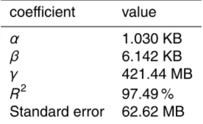
The memory model can be formalised by the following equation:

10

M=α·jpi·jpj·jpk+β·Opt+γ

where jpi, jpj and jpk represent the size of the subdomain along the three dimensions and Opt is the number of ocean points in the subdomain. As in a linear model we can evaluate the coefficientsα,βandγ using a linear regression.

The test configuration used to evaluate the coefficients is executed on 672 processes

15

and, for each one, the total amount of allocated memory was measured. The number of ocean points of each subdomain is evaluated using the bathymetry input file. Figure 11 shows the memory evaluated for the configuration with 672 processes.

Table 6 reports the evaluation of the coefficients obtained with the linear regression, the standard error and the coefficient of determination (R2), which refers to the diff

er-20

ence between the value of memory estimated and measured. It can assume values between 0 and 1. A value of 1 means that there is a perfect correlation, i.e. there is no difference between the estimated value and the actual one. The memory model has been validated with other domain decompositions ranging from 160 to 512 cores (see Fig. 12 as example of comparison between the memory measured for each

pro-25

(17)

GMDD

8, 10585–10625, 2015

I. Epicoco et al.

Title Page

Tables Figures

◭ ◮

Back Close

Full Screen / Esc

Discussion

P

a

per

|

Discussion

P

a

per

|

Discussion

P

a

per

|

Discussion

P

a

per

|

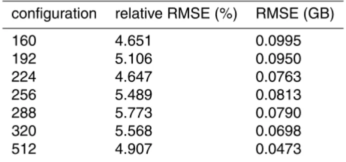
RMSE, instead, expresses the ratio between the root mean square error and the av-erage of the examined sample. The relative RMSE is always less than 6 %, so we can assume that the memory model estimates with a good approximation the actual trend. Figure 13 shows the trend of the memory footprint estimated by the model. The dif-ference between the process with the most allocated memory (red line) and the least

5

allocated memory (blue line) gives also a measure of the load unbalancing, which is greater for the smallest decompositions and decrease (i.e. the computation is better balanced) for the highest decompositions. This can be explained since the highest de-compositions gives smaller subdomains with a number of land points evenly distributed (recall that the subdomains with only land points are excluded from the computation).

10

This test shows also that in a smaller configuration the memory required by each pro-cess is substantially larger and then it is more likely to have an additional time over-head, due to the combination of processes on a node may request more memory than the one available.

7 Conclusions

15

The present work aimed at analysing the computational performance of the PELAGOS coupled model at 0.25◦ of horizontal resolution on two different computing architec-tures, in order to identify the presence of computational bottlenecks and limiting factors to the scalability on many cores architectures. The analysis highlighted three main as-pects limiting the model scalability:

20

– The I/O management. Before starting the scalability analysis, some tests on the two architectures have been performed using the model complete of all of its features. The management of I/O is ine_fficient when the number of processes increases. In fact, the number of the reading/writing files is proportional to the number of processes. On the one hand this peculiarity allows the parallelisation of

25

(18)

GMDD

8, 10585–10625, 2015

I. Epicoco et al.

Title Page

Tables Figures

◭ ◮

Back Close

Full Screen / Esc

Discussion

P

a

per

|

Discussion

P

a

per

|

Discussion

P

a

per

|

Discussion

P

a

per

|

on the other one, the I/O management is prohibitive when we have thousands of processes. For this reason, the I/O has been omitted from the performance analysis, focusing only on the computational aspects. In future, the adoption of more performant I/O strategy will be necessary (e.g., the use of XIOS tool for I/O management).

5

– The memory usage balancing. The presence of the BFM component introduces a load imbalance due to the different number of ocean points belonging to each subdomain. Since the memory allocated by each process is related to the num-ber of ocean points, a balancing strategy of the memory allocated for each node would improve the performance. In this context, some mapping strategies of the

10

processes on the physical cores could be taken into account.

– The communication overhead. PELAGOS is based on a pure MPI parallelisation. When the number of processes increases, the ratio between computation and communication decreases. Beyond a limit, the communication overhead becomes unsustainable. A possible solution is to parallelise along the vertical direction or

15

overlap communications with computation. A hybrid parallelisation strategy can be taken into account, adding for example OpenMP to MPI. This strategy would allow a better exploitation of many-core architectures. Moreover, a further level of parallelism over the state variables treated by the BFM could be introduced.

The work has also demonstrated that the one-dimensional data structure used in

20

BFM, does not affect the performance when compared with the three-dimensional data structure used in NEMO. The workload in BFM is unbalanced since the global do-main is divided among the processes following a block decomposition without taking into account the number of ocean points which fall in a subdomain. The adoption of smarter domain decomposition, e.g. based on the number of ocean points, could lead

25

to a significant improvement of the performance.

(19)

scien-GMDD

8, 10585–10625, 2015

I. Epicoco et al.

Title Page

Tables Figures

◭ ◮

Back Close

Full Screen / Esc

Discussion

P

a

per

|

Discussion

P

a

per

|

Discussion

P

a

per

|

Discussion

P

a

per

|

tists and application domain scientists is a key step to reach substantial improvements toward the full exploitation of next generation computing systems.

Code availability

The PELAGOS025 software is based on NEMO v3.4 and BFM v5.0 both available for download from the respective distribution sites (http://www.nemo-ocean.eu/ and http:

5

//bfm-community.eu/). The software for coupling NEMO v3.4 with BFM v5.0 is available upon request (please contact the BFM System Team – [email protected]). Section 3 of the BFM manual (Vichi et al., 2015a) reports all the details on the coupling. Finally the ORCA025 configuration files used for this work are available upon request to the paper authors.

10

Acknowledgements. The authors thankfully acknowledge the computer resources, technical expertise and assistance provided by the Argonne Leadership Computing Facilities, namely dr. Paul Messina. The authors acknowledge the NEMO and BFM Consortia for the use of the NEMO System and BFM System.

This work was partially founded by EU Seventh Framework Programme within the IS-ENES

15

project [grant number 228203] and by the Italian Ministry of Education, University and Research (MIUR) with the GEMINA project [grant number DD 232/2011].

References

Balaji, V., Redler, R., and Budich, R. G. P. (Eds.): Earth System Modelling 4: IO and Postpro-cessing, Springer, Berlin, Heidelberg, published online, 58, 2013. 10587

20

Balay, S., Gropp, W. D., McInnes, L. C., and Smith, B. F.: Efficient management of parallelism in object oriented numerical software libraries, in: Modern Software Tools in Scientific Comput-ing, edited by: Arge, E., Bruaset, A. M., and Langtangen, H. P., Birkhäuser Press, 163–202, 1997. 10587

Barnier, B., Madec, G., Penduff, T., Molines, J., Treguier, A., Le Sommer, J., Beckmann, A.,

Bi-25

(20)

GMDD

8, 10585–10625, 2015

I. Epicoco et al.

Title Page

Tables Figures

◭ ◮

Back Close

Full Screen / Esc

Discussion

P

a

per

|

Discussion

P

a

per

|

Discussion

P

a

per

|

Discussion

P

a

per

|

and Fichefet, T.: Impact of partial steps and momentum advection schemes in a global ocean circulation model at eddy-permitting resolution, Ocean Dynam., 56, 543–567, 2006. 10590 Blackford, L.S., Choi, J., Cleary, A., Demmel, J., Dhillon, I., Dongarra, J., Hammarling, S., Henry,

G., Petitet, A., Stanley, K., Walker, D., and Whaley, R. C.: ScaLAPACK: a portable linear al-gebra library for distributed memory computers – design issues and performance, in:

Pro-5

ceedings of the 1996 ACM/IEEE conference on Supercomputing, Pittsburgh, Pennsylvania, 17–22 November 1996, 5 pp., 1996. 10587

Claussen, M.: Earth system models, in: Understanding the Earth System: Compartments, Pro-cesses and Interactions, edited by: Ehlers, E., and Krafft, T., Springer, Heidelberg, Berlin, New York, 147–162, 2000. 10586

10

Dennis, J. M. and Loft, R. D.: Refactoring scientific applications for massive parallelism, in: Nu-merical Techniques for Global Atmospheric Models, Lecture Notes in Computational Science and Engineering, edited by: Lauritzen, P., Jablonowski, C., Taylor, M., and Nair, R., Springer, Berlin, Heidelberg, 539–556, 2011. 10587

Dongarra, J., Du Croz, J., Hammarling, S., and Hanson, R. J.: An extended set of

15

FORTRAN basic linear algebra subprograms, ACM T. Math. Software, 14, 1–17, doi:10.1145/42288.42291, 1988. 10587

Dongarra, J., Du Croz, J., Hammarling, S., and Duff, I. S.: A set of level 3 basic linear algebra subprograms, ACM T. Math. Software, 16, 1–17, doi:10.1145/77626.79170, 1990. 10587 Dongarra, J., Beckman, P., Moore, T., et al.: The International Exascale Software Project

20

roadmap, Int. J. High Perform. C., 25, 3–60, doi:10.1177/1094342010391989, 2011. 10586 Epicoco, I., Mocavero, S., and Aloisio, G.: A performance evaluation method for climate coupled

models, in: Proceedings of the 2011 International Conference on Computational Science (ICCS), Singapore, 1–3 June 2011, 1526–1534, 2011. 10588

Lakner, G., Chung, I. H., Cong, G., Fadden, S., Goracke, N., Klepacki, D., Lien, J., Pospiech, C.,

25

Seelam, S. R., and Wen, H. F.: IBM System Blue Gene Solution: Performance Analysis Tools, IBM Redpaper Publication, 2008. 10593

McKiver, W., Vichi, M., Lovato, T., Storto, A., and Masina, S.: Impact of increased grid resolution on global marine biogeochemistry, J. Marine Syst., 147, 153–168, 2015. 10590

Mirin, A. A. and Worley, P. H.: Improving the performance scalability of the community

atmo-30

(21)

GMDD

8, 10585–10625, 2015

I. Epicoco et al.

Title Page

Tables Figures

◭ ◮

Back Close

Full Screen / Esc

Discussion

P

a

per

|

Discussion

P

a

per

|

Discussion

P

a

per

|

Discussion

P

a

per

|

Parashar, M., Li, X., and Chandra, S.: Advanced Computational Infrastructures for Parallel and Distributed Applications (Vol. 66), John Wiley and Sons, 2010. 10592

Reid, F. J. L.: NEMO on HECToR – A dCSE Project, Report from the dCSE project, EPCC and University of Edinburgh, 2009. 10590

Schellnhuber, H. J.: Earth system analysis and the second Copernican revolution, Nature, 402,

5

C19–C23, 1999. 10586

Siedler, G., Griffies, S. M., Gould, J., and Church, J. A.: Ocean Circulation and Climate: A 21st century perspective (Vol. 103). Academic Press, 2013. 10587

Vichi, M. and Masina, S.: Skill assessment of the PELAGOS global ocean biogeochemistry model over the period 1980–2000, Biogeosciences, 6, 2333–2353,

doi:10.5194/bg-6-2333-10

2009, 2009. 10589

Vichi, M., Pinardi, N., and Masina, S.: A generalized model of pelagic biogeochemistry for the global ocean ecosystem. Part I: Theory, J. Marine Syst., 64, 89–109, 2007. 10589

Vichi, M., Gutierrez Mlot, G. C. E., Lazzari, P., Lovato, T., Mattia, G., McKiver, W., Masina, S., Pinardi, N., Solidoro, C., and Zavatarelli, M.: The Biogeochemical Flux Model (BFM):

Equa-15

tion Description and User Manual, BFM version 5.0 (BFM-V5), Release 1.0, BFM Report Series 1, Bologna, Italy, 2015a. 10589, 10593, 10603

Vichi, M., Lovato, T., Gutierrez Mlot, E., and McKiver, W.: Coupling BFM with ocean models: the NEMO model (Nucleus for the European Modelling of the Ocean), Release 1.0, BFM Report Series 2, Bologna, Italy, doi:10.13140/RG.2.1.1652.6566, 2015b. 10589, 10593

20

Washington, W. M.: The computational future for climate change research, J. Phys. Conf. Ser., 16, 317–324, doi:10.1088/1742-6596/16/1/044, 2005. 10586

Washington, W. M.: Scientific grand challenges: challenges in climate change science and the role of computing at the extreme scale, Report from the DOE Workshop, 2008. 10587 Worley, P. H., Craig, A. P., Dennis, J. M., Mirin, A. A., Taylor, M. A., and Vertenstein, M.:

Perfor-25

mance and performance engineering of the community Earth system model, in: Proceedings of the 2011 ACM/IEEE Conference on Supercomputing, Seattle, WA, 12–18 November 2011, Article 54, 2011. 10587

XIOS wiki page: available at: http://forge.ipsl.jussieu.fr/ioserver/, last access: 2 December 2013. 10587, 10591

(22)

GMDD

8, 10585–10625, 2015

I. Epicoco et al.

Title Page

Tables Figures

◭ ◮

Back Close

Full Screen / Esc

Discussion

P

a

per

|

Discussion

P

a

per

|

Discussion

P

a

per

|

Discussion

P

a

per

|

Table 1.Architectures parameters related to the BlueGene/Q (named VESTA), located at the Argonne Leadership Computing Facilities (ALCF/ANL) and the iDataPlex equipped with Intel Sandy Bridge processors (named ATHENA), located at the CMCC.

Design Parameters BG/Q (ANL) IBM iDataPlex (CMCC)

Processor PowerPC A2 Intel Xeon Sandy Bridge

Cores/Node 16 16

Hardware Threads 4 2

Flop/clock/core 8 8

Flop/Node (GFlop) 204.8 332.8

Clock Speed (GHz) 1.6 2.6

RAM/core (GB) 1 4

(23)

GMDD

8, 10585–10625, 2015

I. Epicoco et al.

Title Page

Tables Figures

◭ ◮

Back Close

Full Screen / Esc

Discussion

P

a

per

|

Discussion

P

a

per

|

Discussion

P

a

per

|

Discussion

P

a

per

|

Table 2.Domain decompositions used for the experiments on the Sandy Bridge (Athena) and BG/Q (Vesta) architectures. The first two columns report the number of subdomains along the two horizontal directions, the third column shows the total number of processes excluding the land ones. It follows a column indicating the number of nodes used to run the experiment while the last columns show the average execution time, in s, for a time step of the simulation on both machines.

jpni jpnj jpnij nodes SB

s step−1 BG/Q s step−1

6 29 160 10 25.05 –

38 18 544 34 7.42 –

52 24 944 59 5.27 –

104 17 1344 84 4.78 –

70 34 1728 108 3.19 –

122 23 2048 128 3.27 16.25

363 15 4096 256 – 10.81

281 42 8192 512 – 8.40

(24)

GMDD

8, 10585–10625, 2015

I. Epicoco et al.

Title Page

Tables Figures

◭ ◮

Back Close

Full Screen / Esc

Discussion

P

a

per

|

Discussion

P

a

per

|

Discussion

P

a

per

|

Discussion

P

a

per

|

Table 3.Name and description of the routines selected during the code profiling analyses. The routines identified as belonging to BFM are also the ones that originate from NEMO but they have been modified for the BFM memory structure.

F90 Name Model Tasks

trc_adv, trc_adv_muscl

NEMO Advection of biogeochemical tracers (main caller and specific ad-vection scheme)

calchplus, drtsafe2 BFM Main caller and the iterative scheme to solve the carbonate sys-tem equilibrium using the Newton-Raphson method

tra_qsr NEMO Computation of the temperature trend due to solar radiation pen-etration

div_cur NEMO Computation of horizontal divergence and relative vorticity

dyn_spg_flt, sol_pcg

NEMO Main caller and pre-conditioned conjugate gradient solver for the elliptic differential equation of the surface pressure gradient flux_vector BFM Helper routine that stores the fluxes of material between the BFM

state variables tra_ldf_iso, ldf_slp,

dyn_ldf_bilap

NEMO Horizontal turbulent diffusion for temperature and salinity (along isopycnal levels, with computation of the slope of isopycnals) and momentum

trc_trp_bfm BFM Main caller to advection-diffusion routines for biogeochemical tracers. It loops over the number of BFM state variables and does the remapping between 1-D and 3-D data structuresf microzoodynamics BFM Computation of the reaction terms for microzooplankton

mesozoodynamics BFM Computation of the reaction terms for mesozoplankton tra_zdf_imp NEMO Computation of vertical diffusion of temperature and salinity using

an implicit numerical scheme

phytodynamics BFM Computation of the reaction terms for phytoplankton

pelglobaldynamics BFM Computation of diagnostic terms used in the pelagic model (chlorophyll, nutrient ratios, etc)

pelbacdynamics BFM Computation of the reaction terms for pelagic bacteria

trc_stp NEMO Main caller of the time stepping for biogeochemical tracers. It calls the BFM routines and the transport of biogeochemical trac-ers

zps_hde NEMO Computation of the bottom horizontal gradient for temperature, salinity and density whn using partial steps

tra_sbc, sbc NEMO Surface boundary conditions for temperature and salinity

(25)

GMDD

8, 10585–10625, 2015

I. Epicoco et al.

Title Page

Tables Figures

◭ ◮

Back Close

Full Screen / Esc

Discussion

P

a

per

|

Discussion

P

a

per

|

Discussion

P

a

per

|

Discussion

P

a

per

|

Table 4. Code profiling by applying the HPM (High Performance monitoring Tool) on BG/Q cluster. The first column reports the measured parameters while the other ones show the values on two reference decompositions, respectively on 2048 and 4096 cores.

Measure Values on 2048 cores Values on 4096 cores

Instruction mix FPU=4.49 % FXU=95.51 % FPU=3.01 % FXU=96.99 %

Instructions per cycle/core 0.2548 0.2769

Gflops/Node (Peak 204) 0.598 (Gflops) 0.436 (Gflops) DDR traffic/Node 1.775 (Bytes cycle−1

) 1.168 (Bytes cycle−1 )

Loads that hit in L1 or L1P 98.8 % 99.1 %

MPI Communication time 144.84 (s) 96.72 (s)

(26)

GMDD

8, 10585–10625, 2015

I. Epicoco et al.

Title Page

Tables Figures

◭ ◮

Back Close

Full Screen / Esc

Discussion

P

a

per

|

Discussion

P

a

per

|

Discussion

P

a

per

|

Discussion

P

a

per

|

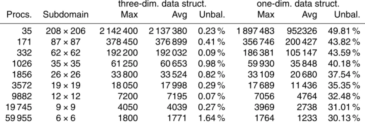
Table 5.Load balancing when adopting the three-dimensional or one-dimensional data struc-ture. The first column reports the number of processes followed by the dimension of the biggest domain. The Max and Avg columns report the maximum number of grid points (i.e. the num-ber of grid points for the biggest domain) and the average value among all the domains. The Unbal. columns give the estimation of the overhead due to unbalancing. It is computed as (Max−Avg)/Max.

three-dim. data struct. one-dim. data struct.

Procs. Subdomain Max Avg Unbal. Max Avg Unbal.

35 208×206 2 142 400 2 137 380 0.23 % 1 897 483 952326 49.81 % 171 87×87 378 450 376 899 0.41 % 356 746 200 427 43.82 % 332 62×62 192 200 192 032 0.09 % 186 381 105 147 43.59 %

1026 35×35 61 250 60 653 0.98 % 59 930 35 848 40.18 %

1856 26×26 33 800 33 524 0.82 % 33 109 20 680 37.54 %

3572 19×19 18 050 17 998 0.29 % 17 689 11 436 35.35 %

9882 12×12 7200 7195 0.07 % 7056 4764 32.48 %

19 745 9×9 4050 4039 0.27 % 3969 2738 31.01 %

(27)

GMDD

8, 10585–10625, 2015

I. Epicoco et al.

Title Page

Tables Figures

◭ ◮

Back Close

Full Screen / Esc

Discussion

P

a

per

|

Discussion

P

a

per

|

Discussion

P

a

per

|

Discussion

P

a

per

|

Table 6.Estimation of the memory model coefficients. The evaluation has been experimentally performed considering a decomposition made of 19×45 subdomains with 183 of them having only land points (672 parallel processes have been used for the simulation).

coefficient value

α 1.030 KB

β 6.142 KB

γ 421.44 MB

R2 97.49 %

(28)

GMDD

8, 10585–10625, 2015

I. Epicoco et al.

Title Page

Tables Figures

◭ ◮

Back Close

Full Screen / Esc

Discussion

P

a

per

|

Discussion

P

a

per

|

Discussion

P

a

per

|

Discussion

P

a

per

|

Table 7. Evaluation of the memory model accuracy. The first column reports the examined decompositions, the last one shows the root mean square error (RMSE), expressed in Giga-Bytes, while the second one shows the relative RMSE expressed as the root mean square error compared with the average of the examined sample.

configuration relative RMSE (%) RMSE (GB)

160 4.651 0.0995

192 5.106 0.0950

224 4.647 0.0763

256 5.489 0.0813

288 5.773 0.0790

320 5.568 0.0698

(29)

GMDD

8, 10585–10625, 2015

I. Epicoco et al.

Title Page

Tables Figures

◭ ◮

Back Close

Full Screen / Esc

Discussion

P

a

per

|

Discussion

P

a

per

|

Discussion

P

a

per

|

Discussion

P

a

per

|

(30)

GMDD

8, 10585–10625, 2015

I. Epicoco et al.

Title Page

Tables Figures

◭ ◮

Back Close

Full Screen / Esc

Discussion

P

a

per

|

Discussion

P

a

per

|

Discussion

P

a

per

|

Discussion

P

a

per

|

(31)

GMDD

8, 10585–10625, 2015

I. Epicoco et al.

Title Page

Tables Figures

◭ ◮

Back Close

Full Screen / Esc

Discussion

P

a

per

|

Discussion

P

a

per

|

Discussion

P

a

per

|

Discussion

P

a

per

|

(32)

GMDD

8, 10585–10625, 2015

I. Epicoco et al.

Title Page

Tables Figures

◭ ◮

Back Close

Full Screen / Esc

Discussion

P

a

per

|

Discussion

P

a

per

|

Discussion

P

a

per

|

Discussion

P

a

per

|

(33)

GMDD

8, 10585–10625, 2015

I. Epicoco et al.

Title Page Abstract Introduction Conclusions References Tables Figures ◭ ◮ ◭ ◮ Back Close

Full Screen / Esc

Printer-friendly Version Interactive Discussion Discussion P a per | Discussion P a per | Discussion P a per | Discussion P a per | 0.90 1.00 1.10 1.20 1.30 1.40 1.50 1.60 1.70 1.80 calch plus ﬂux_v ecto r tra_l df_i so trc_tr p_b fm tra_ad v_m uscl mic rozo odyn am ics mes ozo odyn am ics tra_zd f_im p phyto dynam ics pelg lobal dynam ics drts afe2 pelb acdy nam ics trc_ad v

Spe

e

dup

Main Rou-nes

Rou-ne Speedup on Vesta (@ALCF)

(34)

GMDD

8, 10585–10625, 2015

I. Epicoco et al.

Title Page

Tables Figures

◭ ◮

Back Close

Full Screen / Esc

Discussion

P

a

per

|

Discussion

P

a

per

|

Discussion

P

a

per

|

Discussion

P

a

per

|

0.00 0.20 0.40 0.60 0.80 1.00 1.20 1.40 1.60 1.80

trc_s tp

tra_ad v_m

uscl

sol_p cg

zps_h de _sbc

tra_l df_i

so

tra_zd f_im

p

tra_s bc

tra_ad v

tra_q sr

dyn_s pg_ﬂ

t

ldf_s lp

div_c ur

tra_b bl

dyn_l df_b

ilap

Spe

e

dup

Main Rou-nes

Rou-ne Speedup on Athena (@CMCC)

(35)

GMDD

8, 10585–10625, 2015

I. Epicoco et al.

Title Page

Tables Figures

◭ ◮

Back Close

Full Screen / Esc

Discussion

P

a

per

|

Discussion

P

a

per

|

Discussion

P

a

per

|

Discussion

P

a

per

|

8 16 32 64 128 256 512 1024

16 32 64 128 256 512 1024 2048

Num

be

r of

pr

oc

e

sse

s along j

‐dir

e

c5

on

Number of processes along i‐direc5on

Rela5onship between number of procs along i and j to get squared subdomains

(36)

GMDD

8, 10585–10625, 2015

I. Epicoco et al.

Title Page

Tables Figures

◭ ◮

Back Close

Full Screen / Esc

Discussion

P

a

per

|

Discussion

P

a

per

|

Discussion

P

a

per

|

Discussion

P

a

per

|

1 1.02 1.04 1.06 1.08 1.1 1.12 1.14

32 128 512 2048 8192 32768

Number of processes

Comparison between three‐dimensional and one‐dimensional data structure

(37)

GMDD

8, 10585–10625, 2015

I. Epicoco et al.

Title Page

Tables Figures

◭ ◮

Back Close

Full Screen / Esc

Discussion

P

a

per

|

Discussion

P

a

per

|

Discussion

P

a

per

|

Discussion

P

a

per

|

(38)

GMDD

8, 10585–10625, 2015

I. Epicoco et al.

Title Page

Tables Figures

◭ ◮

Back Close

Full Screen / Esc

Discussion

P

a

per

|

Discussion

P

a

per

|

Discussion

P

a

per

|

Discussion

P

a

per

|

0.00 0.50 1.00 1.50 2.00 2.50 3.00 3.50

16 64 256 1024 4096 16384 65536

Number of processes

Amount of memory w.r.t. the baseline with 1 process

One‐dim

Three‐dim

(39)

GMDD

8, 10585–10625, 2015

I. Epicoco et al.

Title Page

Tables Figures

◭ ◮

Back Close

Full Screen / Esc

Discussion

P

a

per

|

Discussion

P

a

per

|

Discussion

P

a

per

|

Discussion

P

a

per

|