Performance Evaluation of Pro-Active
Routing Protocols with Fading Models: An
Empirical Evaluation using Ns-2
Bilal Maqbool Beigh
Computer Science, university of Kashmir, Srinagar, Hazratbal,190006,India.
Prof, M.A.Peer
Chairman BOPEE, J&K Srinagar,190006,India.
Dr.Mehraj-Din Dar
Director IT&SS, university of Kashmir, Srinagar, Hazratbal,190006,India.
Irshad Ahmad Mir
Computer Science, university of Kashmir, Srinagar, Hazratbal,190006,India.
Suhail Qadir Mir
Computer Science, university of Kashmir, Srinagar, Hazratbal,190006,India.
Abstract:
Almost everything has been done by researchers in performance evaluation of adhoc routing protocols, but under ideal conditions. In previous researches they have carried out analysis based on simplified assumption and unrealistic propagation models. But in evaluating performance of routing protocols the most important factor to be overlooked is change/variation in signal strength, known as fading. The previous researchers had evaluated the performance of routing protocols under simplified and un-realistic propagation models. Thus the choices of selecting propagation models have great impact on the performance analysis. In this paper, comparative analysis will be carried out on the basis of performance evaluation under normal as well as realistic conditions. We will simulate non fading models such as free space and two ray ground for comparison with fading models such as shadowing, Ricean and Rayleigh fading, then accordingly compare the results.The paper is a future of our earlier work reported in [Bilal Maqbool et.al 2010].
Keywords: adhoc networks, fading, protocols, simulate, propagation model, performance, ns-2, DSDV, OSLR, WRP.
1. Introduction:
N (x) N {n | d(x, n } r, x n , j N, j | N |} r x f f f = = ≤≠ ≤
Where x is an arbitrary node in graph G and d is a distance function [10]. A path (route) from node i to node j, denoted by Rij is a sequence of nodes Rij=(i,n1, n2,…,nk, j) where (i,n1), (nk,j) and (ny,ny+1) for 1≤y ≤k-1 are links. A simple path from i to j is a sequence of nodes with no node being repeated more than once. Due to the mobility of the nodes, the set of paths (wireless links) between any pair of nodes and distances is Changing over time. New links can be established and existing links can vanish. The node has to discover the route by route discovery methods and then if there is some topology change, it is done by route maintenance phase. The medium generally used for adhoc routing is radio transmission. There are some obstacles which effects the radio transmission and can be of five categories.
► Reflection.
► Scattering.
► Diffraction.
► Absorption.
► Refraction.
1.1 Reflection:
Reflection is the abrupt change in the direction of a wave front at an interface between two dissimilar media so that the wave front returns into the medium from which it originated.
1.2 Scattering:
Is the mechanism in which the direction of the wave is changed when wave encounters propagation medium discontinuous smaller than the wave length, which results in a random change in the energy distribution.
1.3 Diffraction:
This propagation effect is undergone by a wave when it hits an impenetrable object. The wave bends at the degree of the object, thereby propagating in different directions. This phenomenon is termed as diffraction. The dimensions of the object causing diffraction are comparable to the wavelength of the wave being diffracted. The bending causes by the wave to reach places behind the object which generally cannot be reached by the line of sight transmission.
1.4 Absorption:
Absorption is the conversion of the transmitted electromagnetic energy into another form, usually thermal. The conversion takes place as a result of interaction between the incident energy and the material medium.
1.5 Refraction:
Refraction is redirection of a wave front passing through a medium having a refractive index that is a continuous function of position or through a boundary between two dissimilar media.
2. Premiliries:
2.1 Propagation Models:
signal as well as reflected, scattered and diffracted signal characterizing multipath reception[6][1] also called as multipath propagation. The signals received are called as the multipath waves or multipath signal. The strength of the wave decreases as the distance between the transmitter (T) and receiver (R) increases.
The propagation models are usually characterized as: nonfading and fading. The non-fading propagation
models account for the fact that a radio wave has to cover a growing area when the distance to the sender is increasing. Examples are free-space and two ray ground [4, 11]. On the other hand, fading propagation models calculate the signal strength depending on node’s movements or small time frames. There is signal attenuation due to different objects (large scale fading) as well as variability due to multipath (small scale fading).Large scale fading is characterized by a large distance separating transmitter and receiver, while in small scale fading, the receiver gets multiple copies of a signal which interfere with each other and causes fluctuation is signal strength over a short distance [4]. Several statistical models are used to describe fading in wireless environments and the most frequently used distribution for large scale fading is shadowing, while for small scale fading, Rayleigh, and Ricean [12, 13]can be used. In these models, the instantaneous received power of a given signal may be treated as a stochastic random variable that varies with distance and the selection of a particular model associates a known probability distribution with this random variable.
2.1.1 Non Fading Model:
In non-fading models, the received signal power Pr is calculated for every transmission between two nodes with the chosen propagation model. The channel model distinguishes primarily between three cases. In case Pr is greater than the receiving threshold RXThresh, the transmission has enough power to allow proper reception at the receiver side. Other simultaneous transmissions with reasonable transmission powers may certainly interfere with this transmission and make a correct reception impossible. If Pr is below RXThresh but greater than the carrier sense threshold CSThresh, the receiving node must drop the packet. However, the receiving power of this transmission is still strong enough to interfere with other simultaneous transmissions. Consequently, these interfered packets are also invalid and nodes must drop them as well. Transmissions with receiving powers Pr smaller than CSThresh do not even obstruct other simultaneous transmissions at the same node. Two different propagation models are considered as non-fading: the free space model and the two ray ground models [4, 14, 5].
2.1.1.1 Free Space Model:
The Free Space model represents by equation (1) a signal propagating through open space, with no environmental effects. It has one parameter, called "line of sight". With this parameter off, terrain has no effect on propagation. With it on, the model uses terrain data solely to determine if a line-of-sight (LOS) exists between the transmitting and receiving antennas. If there is no LOS, the signal is blocked entirely and no communication takes place.
Pr = Pt . Gt . Gr. (1) 4 L
Pr the received signal is power (in Watt), Pt Where receiving and the transmitting antennas respectively. is the wave length, L is the system loss, and d is the distance between the transmitter and the receiver. According to [14], a single direct path between the communicating partners exists seldom at larger distances.
2.1.1.2 Two ray model:
The free space model described above assumes that there is only one signal pat from the transmitter to the receiver. But in reality, the signal reaches the receiver through multiple paths (because of reflection, refraction and scattering) the two path model tries to capture this phenomenon. The model assumes that the signal reaches the receiver through two paths, one line of sight path, and the other the path through which the reflected (or refracted, or scattered) wave is received. According to the two path model, the received power is given by
Pr = . . .( (2)
Where Pt is the transmitted power, Gt and Gr represent the antenna gain at the transmitter and the receiver respectively, d is the distance between the transmitter and the receiver, and ht and hr are the heights of the transmitter and the receiver, respectively.
Statistical models are used to accurately predict the fading effect. In large scale fading, the shadowing model shows how the signal strength fades with distance according to power law and reflects the variation of power at a distance. In small scale fading, a fading in which the reflected signal components reaching the receiver are of almost equal strength is called a Rayleigh fading and the one in which there is one principal component that has higher contribution towards signal reception is called Ricean fading. The following is based on [7, 8].
2.1.2.1 Rician:
For fast fading, random variable descriptions are obtained through consideration of the behaviours of the total received fields. Fast fading results due to interference among signals propagating over many paths between transmitter and receiver. Two distinct cases involving fast fading occur: situations in which a dominant line-of-sight path exists between Transmitter and receiver, and situations in which a dominant line-of-site path does not exist. In the former case, multipath reflected fields are added to the direct line-of-sight path, while in the latter, only the multipath signals are received. In both cases we will assume that the number of multipath signals received becomes large, so that the received field, which is a sum of contributions from these paths, approaches a Gaussian random variable. Using time harmonic analysis, we can represent the received field in terms of its real and imaginary components, both of which will be Gaussian random variables. In addition, for a sufficiently large number of multipath terms, the phase of the total of the multipath contributions will be random (excluding the line-of-sight path), so that the real and imaginary field components of the multipath field are independent of one another. The random phase behaviour of the multipath fields implies that the average multipath field received is zero, although significant variations can be observed in a given measurement. Fast fading effects are most conveniently modeled by treating the received power, and not the path loss, as the random variable of interest. In the case with a dominant line-of sight path, we describe the average received power in the absence of fast fading effects as Pm (in Watts, not decibels). The empirical path loss methods along with a statistical model of slow fading (if desired) combined with the Friis formula can be utilized to estimate Pm in a given problem. To model fast fading effects, we assume that an additional fast fading power Pf is added to Pm to obtain the mean power received:
P rec, mean = Pf + Pm ... (3)
again in Watts. It was shown by Rice in 1944 that the appropriate pdf for the total power received is
(P) = 1/ / (2 / )
Which of course applies for p > 0 only. The quantity represents the modified Bessel function of zeroth order; routines and tables for computing this function are widely available. For Pf = 1 Watt and for varying values of Pm in Watts, indicated in the legend. It is not surprising the pdfs are cantered around the value of Pm specified. It is somewhat surprising that the width of the pdf's increases for fixed Pf as Pm is increased. Given the above pdf, the standard deviation of the receiver power can be found to be
P = Pf (Pf + 2Pm) (5)
The inclusion of Pm in this equation confirms the increasing width of the pdf functions as Pm is increased.
2.1.2.2 Rayleigh fading:
The phase of each path can change by 2 radian when the delay changes by . If is large, relative
small motions in the medium can cause change of 2 radians. Since the distance between the devices are much larger than the wavelength of the carrier frequency, it is reasonable to assume that the phase is uniformly distributed between 0 and radians and the phases of each path are independent .When there are large number of paths, applying Central Limit Theorem, each path can be modeled as circularly symmetric complex Gaussian randomvariable with time as the variable. This model is called Rayleigh fading model. A circularly symmetric complex Gaussian random variable is of the form,
Z= X+jY
E[Z] = E[ Z] = E[Z]
The statistics of a circularly symmetric complex Gaussian random variable is completely specified by the variance,
= E[ ]
The magnitude | |which has a probability density is called aRayleigh random variable.
P(z) = e , x>0
This model, called Rayleigh fading model, is reasonable for an environment where there are large number of reflectors.
2.1.2.3 Shadowing Model:
The free space model and the two-ray model predict the received power as a deterministic function of distance. They both represent the communication range as an ideal circle and predict the mean received power at distance “d”. In reality, the received power at certain distance is a random variable due to multipath propagation effects, which is also known as fading effects. A more general and widely-used model is the shadowing model. The shadowing model consists of two parts. The first one is known as path loss model, which predicts the mean received power at distance “d”. It uses a close-in distance “d0“as a reference. Mean received power is computed relative to Pr(d0) as shown below:
= …. Equation 4
Where is called the path loss exponent and is usually empirically determined by field measurement. From Equation 4 we know that = 2 for Free space propagation model. Following table gives some values of . Larger values correspond to more obstructions and hence faster decrease in average received power as distance becomes larger. Pr(d0) can be computed from Equation 1.
Environment
Outdoor
Free space
2
Shadowed
urban area 2.7 to 5
Indoor Line-of-sight
1.6 to 1.8
Obstructed 4 to 6
Table: Values of path loss exponent The path loss is usually measured in dB. So from Equation 4 we have
= -10 log …. equation 5.
The second part of the shadowing is known as log-normal shadowing model. It reflects the variation of the received power at certain distance. It is a log-normal random variable, that is, it is of Gaussian distribution if measured in dB. The overall shadowing model is represented by Equation 6
= -10 ... equation 6
Where XdB is a Gaussian random variable with zero mean and standard deviation dB. dB is called the shadowing deviation and is obtained by measurement. Following table shows some values of dB.
Environment
Office, hard partition
7
Office, hard partition
9.6
Factory, line-of-sight
3 to 6
Factory, obstructed 6.8
Table: Values of shadowing deviation dB
The shadowing model extends the ideal circle model to a richer statistic model: nodes can only probabilistically communicate when they are near the edge of the communication range. Before using the shadowing model the user should select the values of path loss exponent and the shadowing deviation dB according to the simulated environment.[3]
3. Network Simulation:
Network simulator Ns-2.9 allinone is a discrete simulator used for research. ns-2 allows researchers to study Internet protocols and large-scale systems in a controlled environment. Network simulator is used to analyze the impact of mobility and fading on the performances of proactive routing protocols. The simulations contain the common values setting of physical layer of IEEE 802.11b. Other network performance parameters have been chosen such that real communication environment is depicted more accurately.[9]
3.1 Simulation Methodology:
Here in this paper, we are considering the parameter as propagation model for performance analysis of proactive routing protocols. We have two types of propagation models first non-fading model and fading model that we discuss above. We are going to evaluate the performance of proactive routing protocols first under non-fading models and then under fading models. In fading models we change the node’s mobility and the result is evaluated under two scenarios, 1). With varying node’s speed 2). With node’s pause time. The node will move randomly varying their speed from minimum to maximum. Also one more thing is considered to be random that is traffic pattern. The movement model will define the active route throughout the entire evaluation simulation time. In each simulation there are 25 source nodes, 25 receiver nodes and the transmission rate is 512 bytes and the simulation time is 200 s. This is necessary in order to enable fair comparisons among the routing protocols and to expose them to identical environmental conditions.
3.2 Performance matrices:
The evaluation of performance of routing protocols can be considered under the below matrices:
► End to End delay.
► Packet Ratio Delivery.
► Routing Overhead.
3.2.1 End to End Delay:
The concept “end-to-end” is used as a relative comparison with “hop-by-hop”. Data transmission seldom occurs only between two adjacent nodes, but via a path which may include many intermediate nodes. End-to-end delay is the sum of delays experienced at each hop from the source to the destination. The delay at each intermediate node has two components: a fixed delay which includes the transmission at sender node and the propagation
over the link to the next node, and a variable delay which includes the processing and queuing at sender node. The propagation delay is the delay in transmitting the data packet along a physical link.
3.2.2 Packet Delivery Fraction (PDF):
PDF also known as the ratio of the data packets delivered to the destinations to those generated by the CBR sources. The PDF shows how successful a protocol performs delivering packets from source to destination. The higher for the value give use the better results. This metric characterizes both the completeness and correctness of the routing protocol also reliability of routing protocol by giving its effectiveness.
PktDelivery% = ∑∑ R
R x
Routing Overhead:
Routing overhead, is the number of control packets transmitted per data packet delivered at the destination. Each hop-wise transmission of a control packet is counted as one transmission. The total number of control packets is calculated by number of route requests, route replies, and route errors of each protocol.
4. Simulation results:
The goal of the paper is to evaluate the impact of different propagation model on the performance of two proactive based routing protocols, while evaluating the performance; we introduce fading effects so that we can get real time environment evaluation. In this paper we are comparing the results of non-fading model with fading models. The result of the simulation performed is based on the three previously defined matrices. Simulation is carried out on two scenarios.
1. Varying node’s pause time. 2. Varying pause time.
4.1 Scenario 1: Performance with varying node’s maximum speed.
DSDV and OSLR show different behaviours at different levels , As speed increases, DSDV delivers less packets and exhibits more delay and more routing overhead than OSLR, as shown in the following figures.
4.1.1. Packet delivery ratio:
The packet delivery ratio decreases with the increase of speed, which implies that the links are relatively stable and more reliable at lower speed. OSLR delivers more packets than DSDV as shown in Fig. 1(a). The main reason for packet drops in wireless ad hoc routing protocols are mobility, congestion, and characteristics of wireless channel. Free space, shadowing and two ray ground models deliver more packets than Rayleigh and Ricean models when packet delivery ratio is considered as metric. The fading models deteriorate the network performance significantly, with Rayleigh and Ricean exhibiting the worst performance. This is due to a random drop in signal strength which causes packets being lost on reliable links, falsely indicating that links have failed, leading to interruption and the need for establishment of new route. This would also increase both delay and routing overhead. As speed increases, DSDV exhibits more delay and more routing overhead than OSLR.
4.1.2. End-to-end delay
DSDV exhibits more delay than OSLR under all speed variations and delay increases with the increase of speed as indicated in Fig. 2(a). In comparison to free space and shadowing, the two ray ground, Rayleigh and Ricean models show higher delay. As expected Ricean model and Rayleigh exhibit more delay than the non-fading models. The abnormality of graphs may be due to higher congestion and increased MAC retries caused by unreliable routes that enforce on demand routing protocols to spend a significant number of their time performing route updates.
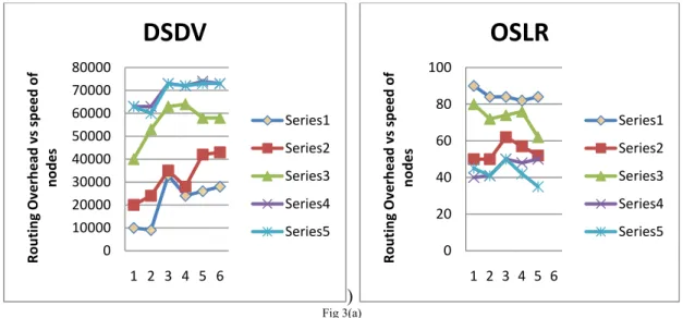
4.1.3. Routing overhead
lot of packets are dropped and updated each time the topology changes. This can be attributed to the constructive interference phenomena due to multipath signal propagation. In free space model, a sharp increase was observed in the routing overhead as the speed increases and this is essentially due to frequent link breaks. A similar behaviour was obtained for two ray ground model, with OSLR performing better than DSDV. In fading model, the two protocols have higher routing overhead compared with non-fading models as indicated in Fig. 3(a). This can be attributed to higher congestion and high inter-nodal interference.
4.2 Scenario 2: Performance with varying node’s pause time.
OSLR and DSDV show an approximately similar behaviour at different levels of pause time when considering packet delivery ratio. As pause time increases, DSDV exhibits more delay and more routing overhead than OSLR as shown in the following figures.
4.2.1. Packet delivery ratio
The two protocols relatively do the same performance when packet delivery ratio over a variety of pause time, for two ray ground, Rayleigh and Ricean models, while free space model exhibits the highest packet delivery ratio as presented in Fig. 4. The lowest delivery ratio is for Ricean model, it is a consequence of the random variations in received signal strength. Packets are lost on a reliable link, falsely indicating that the link has failed leading to the interruption in protocol operation and initiates the need for a new path which would also increase delay and routing overhead. The results indicate that under Ricean and Rayleigh models, DSDV drops more packets than OSLR over a variety of pause times..
4.2.2. End-to-end delay
The two protocols show similar results with DSDV showing higher delay than OSLR as presented in Fig. 5. As expected the highest delay is for fading propagation models.
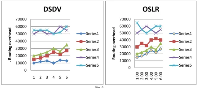
4.2.3. Routing overhead
The routing overhead for Ricean and Rayleigh is high compared to other models with free space which exhibited lowest routing overhead. As pause time increases, the routing overhead decreases, however, under higher pause time the routing overhead starts to increase. When modeled under the Ricean and Rayleigh fading, two protocols show an approximately similar behaviour at different levels of pause time with DSDV performing worse than OSLR as indicated in Fig. 6.
5. Conclusion:
In this paper, the effects of different propagation models on the performance of ad hoc networks have been investigated From the simulation results, the choice of propagation models have a great impact on performance of the routing protocol, so realistic and representative propagation models are necessary as far as the accurate Evaluation of the performance of routing protocols is concerned. The simulation results revealed that the different propagation models affected the performance of the mobile ad hoc network considerably. Consequently, different performance evaluation results were obtained. The performance has deteriorated very quickly when fading models were taken into account; for shadowing, Rayleigh, and Ricean models. The main reasons for this deterioration resulted from the large variation of the received signal strength.
References:
[1] Neskovic, N. Neskovic, and G. Paunovic, “Modern Approaches in Modeling of Mobile Radio Systems Propagation Environment,” IEEE Communications Surveys, Third Quarter 2000.
[2] Bilal Maqbool Beigh, Prof.M.A.Peer.” Classification of Current Routing Protocols for Ad Hoc Networks - A Review”. International Journal of Computer Applications (0975 – 8887) Volume 7– No.8, October 2010.
[3] Exploring Network simulator 2 by Manasa S.Mohit P. Tahiliani
[4] Guardiola IG, Matis TI. Fast-fading, an additional mistaken axiom of wireless-network research. Int J Mobile Network Des Innovation 2007; 2(3–4):153–8.
[5] Hasti AhleHagh. Techniques for communications and geolocation using wireless adhoc networks. Master of science thesis, Worcester Polytechnique institute; 2004
[6] J-P. Linnartz, “Narrowband Land-Mobile Radio Networks,” Artech House, 1993
[7] Lenders, Wagner J, May M. Analyzing the impact of mobility in adhoc networks.ACM/Sigmobile Workshop on Multi-hop Ad Hoc Networks: from Theory to Reality (REALMAN), Italy; 2006.
[8] Nasri Amir, Schober Robert, Ma Yao. Unified asymptotic analysis of linearly modulated signals in fading, non-Gaussian noise, and interference. IEEE Trans Commun 2008; 56(6):980–90.
[10] N. Nikaein, H. Labiod, and C. Bonnet. DDR-Distributed Dynamic Routing Algorithm for Mobile Ad hoc Networks. First Annual Workshop on Mobile and Ad Hoc Networking and Computing (MobiHOC), 2000.
[11] Puccinelli D, Haengi M.Multipath fading in wireless sensor network: measurements and interpretation IEE/ACM international wireless communication and mobile computing conference (IWCMC 06) 2006.
[12] Punnoose NR, Stancil D. Efficient simulation of Ricean fading within a packet simulator. In: Proceedings of IEEE vehicular technology conference; 2000. p. 764–767.
[13] Schmitz A, Wenig M. The effect of the radio wave propagation model in mobile ad hoc networks. In: Proceedings of ACM MSWiM; 2006.
[14] Sridhana V, Bohacek S. Realistic propagation simulation of urban mesh networks. University of Delaware, Department of Electrical and Computer Engineering, Technical Report; 2006.
[15] T. Rappaport, “Wireless Communications: Principles and Practices (2nd edition),” Prentice Hall, 2002 [16] Wreless Communications & Networks By William Stallings -Second Edition
Note:
Series 1= free model, Series 2= shadowing model, Series 3= Two ray model, Series 4= Rician model, Series5= Rayleigh model 1 = 4 m/sScenario 1
: Performance with varying node’s maximum speed.
Fig 1(a) Fig 2(a) 0 20 40 60 80 100 120 1. 00 2. 00 3. 00 4. 00 5. 00 6. 00 Pac k et Delivery Rat io(P D R)
DSDV
Series1 Series2 Series3 Series4 Series5 0 20 40 60 80 100 120 1. 00 2. 00 3. 00 4. 00 5. 00 6. 00 Pac k et Delivery Rat io(P D R)OSLR
Series1 Series2 Series3 Series4 Series5 0 10000 20000 30000 40000 50000 60000 70000 800001 2 3 4 5 6
End to En d Delay Vs Speed (m /s )
DSDV
Series1 Series2 Series3 Series4 Series5 0 20 40 60 80 1001 2 3 4 5 6
)
Fig 3(a)Scenario 2
: Performance with varying node’s pause time.
Fig. 4 Fig. 5 0 10000 20000 30000 40000 50000 60000 70000 80000
1 2 3 4 5 6
Ro ut ing Ov erh e ad vs speed of nod e s
DSDV
Series1 Series2 Series3 Series4 Series5 0 20 40 60 80 1001 2 3 4 5 6
Ro ut ing Ov erh e ad vs speed of nod e s
OSLR
Series1 Series2 Series3 Series4 Series5 0 10 20 30 40 50 60 70 80 90 1001.00 2.00 3.00 4.00 5.00 6.00
Pa ck et Delivery Ra ti o(P D R)
DSDV
Series1 Series2 Series3 Series4 Series5 0 10 20 30 40 50 60 70 80 90 1001.00 2.00 3.00 4.00 5.00 6.00
Pa ck et Delivery Ra ti o(P D R)
OSLR
Series1 Series2 Series3 Series4 Series5 0 500 1000 1500 20001 2 3 4 5 6
End to end dela y )
DSDV
Series1 Series2 Series3 Series4 Series5 0 500 1000 1500 20001.00 2.00 3.00 4.00 5.00 6.00
Fig. 6 0
10000 20000 30000 40000 50000 60000 70000
1 2 3 4 5 6
.
Rou
ti
n
g
ov
erhea
d
DSDV
Series1
Series2
Series3
Series4
Series5
0 10000 20000 30000 40000 50000 60000 70000
1.00 2.00 3.00 4.00 5.00 6.00
Ro
u
ti
n
g
ov
er
hea
d
OSLR
Series1
Series2
Series3
Series4