Extracting Attractive Local-Area Topics in Georeferenced Documents using a New Density-based Spatial Clustering Algorithm

(1)

Extracting Attractive Local-Area Topics

in Georeferenced Documents using

a New Density-based Spatial Clustering Algorithm

Tatsuhiro Sakai, Keiichi Tamura, and Hajime Kitakami

Abstract—Along with the popularization of social media, huge numbers of georeferenced documents (which include location information) are being posted on social media sites via the Internet, allowing people to transmit and collect geo-graphic information. Typically, such georeferenced documents are related not only to personal topics but also to local topics and events. Therefore, extracting “attractive” areas associated with local topics from georeferenced documents is currently one of the most important challenges in different application domains. In this paper, a novel spatial clustering algorithm for extracting “attractive” local-area topics in georeferenced documents, known as the(ǫ, σ)-density-based spatial clustering

algorithm, is proposed. We defined a new type of spatial cluster called an (ǫ, σ)-density-based spatial cluster. The proposed

density-based spatial clustering algorithm can recognize both semantically and spatially separated spatial clusters. Therefore, the proposed algorithm can extract “attractive” local-area topics as (ǫ, σ)-density-based spatial clusters. To evaluate our

proposed clustering algorithm, geo-tagged tweets posted on the Twitter site were used. The experimental results showed that the

(ǫ, σ)-density-based spatial clustering algorithm could extract

“attractive” areas as the (ǫ, σ)-density-based spatial clusters

that were closely related to local topics.

Index Terms—density-based clustering, spatial cluster, DB-SCAN, social media, local topic extraction.

I. INTRODUCTION

I

N recent years, with increasingly widespread use of smart phones equipped with GPS technology and increasing interest in social media, huge numbers of georeferenced documents (which include location information) are being posted on social media sites through the Internet, allowing people to transmit and collect information related to location [1], [2]. Typically, such georeferenced documents are related closely not only to personal topics but also to local topics and events. Therefore, extracting information about local topics and events from georeferenced documents [3] can contribute to different geo-location application domains, such as local area marketing, tourism informatics, and local topic recommendation.

Researchers interested in knowledge discovery through the study of georeferenced documents posted on social media sites have made considerable efforts to tackle the new challenges facing extraction of local topics and events

T.Sakai is with Graduate School of Information Sciences, Hiroshima City University, 3-4-1, Ozuka-Higashi, Asa-Minami-Ku, Hiroshima 731-3194 Japan, corresponding e-mail: my67011@edu.ipc.hiroshima-cu.ac.jp

K.Tamura is with Graduate School of Information Sciences, Hiroshima City University, 3-4-1, Ozuka-Higashi, Asa-Minami-Ku, Hiroshima 731-3194 Japan, corresponding e-mail: ktamura@hiroshima-cu.ac.jp

H.Kitakami is with Graduate School of Information Sciences, Hiroshima City University, 3-4-1, Ozuka-Higashi, Asa-Minami-Ku, Hiroshima 731-3194 Japan, corresponding e-mail: kitakami@hiroshima-cu.ac.jp

from georeferenced documents. For example, dense areas, in which many georeferenced documents including a given keyword are posted, are hot areas of local topics related to that keyword. For example, Crandall et al. [4] developed an algorithm for identifying hot sites and landmarks from geo-tagged photos posted on the Flickr site, one of the most famous photo-sharing sites. Similarly, Sakaki et al. [5] focused on tweets posted on the Twitter site regarding typhoons and earthquakes, using the associated geographic information to estimate typhoon trajectory and earthquake epicenter using dense areas.

We have been developing a new spatial clustering al-gorithm that extracts “attractive” local-area topics, which are semantically-/locally-dense areas in which many relevant georeferenced documents that include keywords relevant to topics are posted [6]. To extract attractive local-area topics, we defined a new type of spatial cluster, which we term a (ǫ, σ)-density-based spatial cluster. This type of cluster is both spatially and semantically separated from other spa-tial clusters. Thus, (ǫ, σ)-density-based spatial clusters are closely related to local topics.

The main contributions of this study are as follows.

• To extract(ǫ, σ)-density-based spatial clusters, we

pro-pose a new spatial clustering algorithm for georefer-enced documents, termed the(ǫ, σ)-density-based spa-tial clustering algorithm, which is a natural extension of a density-based spatial clustering of applications with noise (DBSCAN) [7]. DBSCAN is a basic density-based spatial clustering algorithm based on neighborhood den-sity and can recognize areas in which denden-sity is higher than that of the surrounding areas. However, it does not take into account similarities between the contents of georeferenced documents. Conversely, the (ǫ, σ)-density-based spatial clustering algorithm can recognize (ǫ, σ)-density-based spatial clusters, which are both semantically and spatially separated from other spatial clusters.

• To recognize semantically/spatially separated clusters as

(ǫ, σ)-density-based spatial clusters, we defined a new similarity measurement for georeferenced documents on social media sites. On such sites, users typically post georeferenced documents comprising short messages including a local topic. Therefore, if georeferenced documents include the same keyword, they can be considered similar to each other. On the basis of this concept, we define a new similarity measurement based on a keyword-based Simpson’s coefficient.

• To evaluate the proposed density-based spatial

(2)

actual data set consisting of 480,000 tweets from the Twitter site; these were posted from November 2011 to February 2012. We confirmed that the(ǫ, σ)-density-based spatial clustering algorithm could extract(ǫ, σ)-density-based spatial clusters that represent “attractive” areas associated with local topics.

The remainder of this paper is organized as follows. In Section 2, related work is reviewed. In Section 3, the(ǫ, σ)-density-based spatial cluster is defined. In Section 4, the (ǫ, σ)-density-based spatial clustering algorithm is described. In Section 5, the results of an evaluation using tweets posted on Twitter are presented. Finally, some concluding remarks are presented in Section 6.

II. RELATEDWORK

The popularization of smart phones equipped with GPS technology has opened up entirely new types of data that can be sourced from social media sites. For example, referenced data, which include both the location (e.g., geo-tag, address, and landmark name) and time of the post, can now be collected. In this context, users on social media sites are referred to as sensors that observe the real world as it happens around them, and georeferenced data can be considered sensor data that describe topics and events in the real world [8].

Since the use of the Internet has become widespread, topic detection and tracking in online documents [9] have become some of the most attractive research topics in many application domains, with many new types of document becoming available. For example, geo-tagged tweets on the micro-blogging site Twitter can be used as georeferenced documents for extracting topics and events. Geo-tagged photos on the Flickr site also are focused on from many researchers and practitioners to identify areas related to local topics and events.

The majority of previous studies investigating georefer-enced data have adopted DBSCAN, a density-based spatial clustering algorithm [7], [10]. The shapes of spatial clus-ters in geo-spatial data typically exhibit various forms, and some spatial clusters may be completely surrounded by (but not connected to) other clusters. To extract such arbitrarily shaped clusters, density-based spatial clustering algorithms must focus on high-density areas in data space, which are separated by areas of lower density. DBSCAN was originally (and in subsequent studies) applied to extract specific areas related to local topics and events from geo-spatial data.

Recently, Tamura et al. [11] proposed a novel density-based spatiotemporal clustering algorithm that can extract spatially and temporally separated clusters in georeferenced documents. Their proposed algorithm integrates spatioral criteria into DBSCAN to separate spatial clusters tempo-rally. Similarly, Kisilevich et al. [12] proposed P-DBSCAN, a new density-based spatial clustering algorithm based on DBSCAN, for analysis of attractive places and events using a collection of geo-tagged photos. In particular, they defined a new density measure according to the number of people in a given neighborhood. Our work is similar in nature to these previous studies, although P-DBSCAN and the density-based spatiotemporal clustering algorithm cannot recognize semantically separated spatial clusters; the present study aims to address this shortfall.

Some previous studies investigating clustering techniques for the extraction of topics and events have focused on geo-tagged tweets posted on the Twitter site and image data posted on the Flickr site. For example, Watanabe et al. [13] identified locations that were attracting current attention. Lee et al. [14] developed a method of detecting local events using spatial partitions by separating their entire study area into sub-areas using a Voronoi diagram; then, the developed method recognized the sub-areas in which the number of posted tweets was increasing. Jaffe et al. [15] developed a hierarchical spatial clustering algorithm based on location information for geo-tagged image data posted on the Flickr site. Rattenbury et al. [16] also proposed an identification method of event places for geo-tagged image data posted on Flickr, with the added advantage that their method was able to predict the contents of events using tag data. Subsequently, Yanai et al. [17] applied k-means clustering to geo-tagged image data, and Kim et al. [18] introduced mTrend, which constructs and visualizes spatiotemporal trends of topics, referred to as “topic movements.”

However, these previous studies focused only on spatial clustering using location information, whereas our study focuses on both spatially and semantically separated spa-tial clustering. Moreover, we define a new similarity mea-surement based on a keyword-based Simpson’s coefficient. Extracting semantically-/locally-dense areas allows users to identify local topics, which have received many attention in local area. This study contributes to local area marketing, tourism informatics, and local topic recommendation.

III. (ǫ, σ)-DENSITY-BASEDSPATIALCLUSTER

In this section, the definitions of (ǫ, σ)-density-based spatial criteria and (ǫ, σ)-density-based spatial cluster are presented.

A. Density-based Spatial Criteria

In density-based spatial clustering algorithms, spatial clus-ters are dense areas that are separated from areas of lower density. In other words, areas with high densities of data points can be considered spatial clusters, whereas those with low density cannot. The key concept underpinning the use of density-based spatial clustering algorithms indicates that, for each data point within a spatial cluster, the neighborhood of a user-defined radius must contain at least a minimum number of points; that is, the density in the neighborhood must exceed some predefined threshold.

In DBSCAN, theǫ-neighborhood of a data point is defined as documents in the neighborhood of a user-defined given radiusǫ. Then, theǫ-neighborhood of a data point in a spatial cluster must contain at least a minimum number of data points. In this study, georeferenced documents are utilized as data points and the definition of theǫ-neighborhood of a georeferenced document is extended: we define the (ǫ, σ)-neighborhood of a georeferenced document to extract its semantically similar neighbors.

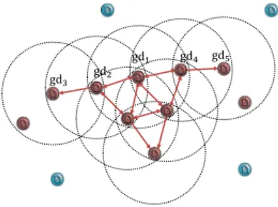
Definition 1 ((ǫ, σ)-neighborhoodGN(ǫ,σ)(gdp)) The

(ǫ, σ)-neighborhood of a georeferenced document gdp, denoted byGN(ǫ,σ)(gdp), is defined as

GN(ǫ,σ)(gdp) ={gdq∈GDS|dist(gdp, gdq)≤ǫ and

(3)

ε

gdp

ε feature vector space

σ

ଷ ସ

gdp gdp

geo-coordinate space geo-coordinate space

ଵ ଶ

ଶ ଵ

ሺகǡ஢ሻ ൌ ͵ க ൌ Ͷ

Fig. 1. Example of definition 1.

where the function dist returns the distance between geo-referenced documentgdpand georeferenced documentgdq, and the functionsimreturns the similarity betweengdpand gdq. The functionsimis explained in the following section.

An example of the ǫ-neighborhood of gdp is shown on the left side of Fig. 1. Theǫ-neighborhood ofgdpis a set of georeferenced documents that exist withinǫfromgdp. In this example, there are four georeferenced documents in the ǫ-neighborhood ofgdp. An example of the(ǫ, σ)-neighborhood of gdp is shown on the right side of Fig. 1. The (ǫ, σ)-neighborhood of gdp is a set of georeferenced documents existing within distance ǫ from gdp and the similarity be-tween each georeferenced document andgdpis greater than a given value of σ. In this example, there are three geo-referenced documents: GN(ǫ,σ)(gdp) = {gd2, gd3, gd4}. A

georeferenced documentgd1is withinǫfromgdp; however, it is not inGN(ǫ,σ)(gdp), because the similarity betweengd1

andgdpis less than than the given value ofσ.

Definition 2 (Core/Border Georeferenced Document) A document gdp is known as a core georeferenced document if there are at least a minimum number of georeferenced documents, M inDoc, in the (ǫ, σ)-neighborhood GN(ǫ,σ)(gdp) (GN(ǫ,σ)(gdp) ≥ M inDoc).

Otherwise, (GN(ǫ,σ)(gdp) < M inDoc), gdp is called a

border georeferenced document.

σ ଷ ଶ

ସ

ଷ ଶ

ସ

gdp gdp

σ ଶ

ଷ

ଶ

ଷgdp

gdp

geo-coordinate space geo-coordinate space ଵ

ଵ

ହ

ሺகǡ஢ሻ ൌ ͵ ሺகǡ஢ሻ ൌ ʹ

Fig. 2. Example of definitions 2 and 3.

Suppose that M inDoc is set to three. A georeferenced document gdp on the left side of Fig. 2 is a core

geo-referenced document, because there are three documents in GN(ǫ,σ)(gdp). Conversely, a georeferenced documentgdpon

the right side of Fig. 2 is a border georeferenced document because the number of documents in GN(ǫ,σ)(gdp) is less

thanM inDoc.

Definition 3 ((ǫ, σ)-density-based directly reachable) Suppose that a georeferenced document gdq is in the (ǫ, σ)-neighborhood ofgdp. If the number of georeferenced documents in the(ǫ, σ)-neighborhood of gdpis greater than or equal toM inDoc, i.e., ifGN(ǫ,σ)(gdp)≥M inDoc,gdq

is(ǫ, σ)-density-based directly reachable fromgdp. In other words, georeferenced documents in the(ǫ, σ)-neighborhood of a core georeferenced document are (ǫ, σ)-density-based directly reachable from the core georeferenced document.

On the left side of Fig. 2, document gdp is a core geo-referenced document, because GN(ǫ,σ)(gdp) ≥ M inDoc.

Georeferenced documentsgd2,gd3andgd4are in the(ǫ, σ)-neighborhood of gdp. These three documents are (ǫ, σ)-density-based directly reachable from gdp. Conversely, on the right side of Fig. 2, document gdp is a border georef-erenced document, i.e., does not conform to the relationship GN(ǫ,σ)(gdp) ≥ M inDoc. These two georeferenced

doc-uments are not (ǫ, σ)-density-based directly reachable from gdp, although georeferenced documentgd2 and gd3 are in the(ǫ, σ)-neighborhood of gdp.

ଵ ଶ ଷ

ହ ସ

Fig. 3. Example of definitions 4 and 5.

Definition 4 ((ǫ, σ)-density-based reachable) Suppose that there is a georeferenced document sequence (gd1, gd2, gd3,· · ·, gdn) and the (i + 1)-th georeferenced

document gdi+1 is (ǫ, σ)-density-based directly reachable from the i-th georeferenced document gdi. The

georeferenced document gdn is (ǫ, σ)-density-based

reachable fromgd1.

An example of an(ǫ, σ)-density-based reachable is shown in Fig. 3. Here, ifM inDoc= 3,gd2 is(ǫ, σ)-density-based directly reachable from gd1 and gd3 is (ǫ, σ)-density-based directly reachable from gd2. The georeferenced document gd3 is (ǫ, σ)-density-based reachable fromgd1. Conversely, gd5 is not(ǫ, σ)-density-based reachable fromgd3, i.e.,gd2 is not(ǫ, σ)-density-based directly reachable fromgd3.

Definition 5 ((ǫ, σ)-density-based connected) Suppose that georeferenced documents gdp and gdq are (ǫ, σ)-density-based reachable from document gdo. If GN(ǫ,σ)(gdo) ≥ M inDoc, it can be stated that gdp is

(4)

An example of an(ǫ, σ)-density-based reachable is shown in Fig. 3. In this figure,gd3is(ǫ, σ)-density-based reachable fromgd1andgd5is(ǫ, σ)-density-based reachable fromgd1. In this instance,gd3is(ǫ, σ)-density-based connected togd5.

B. Definition of Cluster

An (ǫ, σ)-density-based spatial cluster consists of two types of document: core georeferenced documents, which are mutually (ǫ, σ)-density-based reachable; and border georef-erenced documents, which are (ǫ, σ)-density-based directly reachable from the core georeferenced documents. An(ǫ, σ)-density-based spatial cluster is defined as follows.

Definition 6 ((ǫ, σ)-density-based spatial cluster)

An (ǫ, σ)-density-based spatial cluster (DSC) in a georeferenced document set GDS satisfies the following restrictions.

（1） ∀gdp, gdq ∈ GDS, if and only if gdq is (ǫ, σ)-density-based reachable from gdp, gdq is also in DSC.

（2） ∀gdp, gdq ∈ DSC, gdp is (ǫ, σ)-density-based connected togdq.

Even if gdp and gdq are border georeferenced documents, gdp and gdq are in the same (ǫ, σ)-density-based spatial cluster if gdpis(ǫ, σ)-density-based connected togdq.

IV. (ǫ, σ)-DENSITY-BASEDSPATIALCLUSTERING

ALGORITHM

In this section, the proposed (ǫ, σ)-density-based spatial clustering algorithm is described.

A. Data Model

Let gdi denote the i-th georeferenced document in

GDS={gd1,· · ·, gdn}. Then,gdi consists of three items:

gdi =< texti, pti, pli>, where texti is the content (e.g.,

title, short text message, and tags), pti is the time when

the geo-spatiotemporal document was posted, andpli is the

location where gdi was posted or is located (e.g., latitude

and longitude).

B. Algorithm

The algorithm of(ǫ, σ)-density-based spatial clustering is represented by Algorithm 1. In this algorithm, the function IsClustered checks whether document gdp is already as-signed to a spatial cluster. Then, the function GetNeigh-borhood returns the (ǫ, σ)-neighborhood of georeferenced document gdp. For each georeferenced document gdp in GDS, the following steps are executed. If gdp is a core georeferenced document according to Definition 2, it is assigned to a new spatial cluster, and all the neighbors are assigned to a candidate queue CQ for further processing. The functionMakeNewClustermakes a new spatial cluster. The processing and assignment of georeferenced documents to the current spatial cluster continue until CQ is empty. The next georeferenced document is dequeued from CQ. The dequeued georeferenced document is assigned to the current spatial cluster, assuming that this has not been achieved already. Then, the (ǫ, σ)-neighborhood of the de-queued georeferenced document are de-queued toCQusing the function EnNniqueQueue, which puts input georeferenced documents into CQif they are not already inCQ.

input :GDS - georeferenced document set,ǫ -neighborhood radius,σ- similarity rate, M inDoc- threshold value

output:DSC - set of clusters

cid←1; DSC←φ;

fori←1 to|GDS| do gdp←gdi∈GDS;

ifIsClustered(gdp)==f alsethen

GN←GetNeighbors(gdp,ǫ,σ);

if|GN| ≥M inDocthen

stccid←MakeNewCluster(cid,gdp);

cid←cid+ 1;

EnQueue(CQ,GN);

whileCQis not emptydo

gdp←DeQueue(CQ);

GN← GetNeighbors(gdp,ǫ,σ);

if|GN| ≥M inDocthen

EnNniqueQueue(CQ,GN);

end

stccid←stccid∪gdp

end

DSC←DSC∪stccid;

end end end

returnDSC;

Algorithm 1: (ǫ, σ)-Density-based Spatial Clustering Algorithm

C. Keyword-based Similarity Function

Let dti denote all words in texti of the i-th

georefer-enced document: dti = {wi,1, wi,2,· · ·, wi,nw(i)}, where wi,j ∈ W, and W is a set of all words included in {text1, text2,· · ·, textn}. In this study, morphological

anal-ysis was used to extract noun, verb, and adjective phrases as words. Simpson’s coefficient has a feature of cosine similarity for similarity between sets, and the word-based Simpson’s coefficient is defined as follows:

wsim(gdi, gdj) =

|dti∩dtj| |min(dti, dtj)|

. (2)

The word-based Simpson’s coefficient does present some drawback, such as when keywords are broadly the same but several words are different between particular georef-erenced documents. For example, suppose that there are two georeferenced documents gd1 and gd2 that are related to “Itsukushima Shrine.” If dt1 ={“Itsukushima Shrine”, “beautif ul”, “historical”, “Hiroshima”} and dt2 =

{“Itsukushima Shrine”,“wonderf ul”,“sea”,“clean”}, the similarity between two georeferenced documents is wsim(gd1, gd2) = 1/4 = 0.25. In this case, the similarity betweengd1andgd2is low, even thoughgd1andgd2 cover the same topic (i.e., “Itsukushima Shrine”).

(5)

TABLE I

CLUSTERING RESULTS USINGDBSCANINHIROSHIMA

No Number of Tweets Range (longitude) Range (latitude) Top- 5 Frequent Words

1 2173 132.34259769 – 132.5139095 34.34225649 – 34.41800308 shop, inside, today, station, come

2 288 132.301779 – 132.32664956 34.291072 – 34.317351 Miyajima, Itsukushima Shrine, Miyajimaguchi, oyster, ferry

3 170 132.4580275 – 132.4968043 34.43618755 – 34.48192577 shop, day, lunch, AEON MALL Hiroshima Gion, come

4 128 132.90427752 – 132.91733343 34.331726 – 34.348506 Tamayura, station, cat, Mr/Ms, Okonomiyaki

5 97 132.54589487 – 132.57154524 34.2343527 – 34.25657546 Yamato, museum, center, shop, noodle

6 96 132.7203672 – 132.75817651 34.4141014 – 34.43534496 Geso, person, today, set menu, shop

7 86 132.5285826 – 132.54099838 34.3442324 – 34.3628074 Mr/Ms, senaponcoro, shop, buy, seem

8 67 132.30352202 – 132.31108951 34.35173988 – 34.35770497 octopus, ball, while, open, today

TABLE II

CLUSTERING RESULTS USING THE WORDS-BASED METHOD INHIROSHIMA

1 97 132.4572834 – 132.46863105 34.389778 – 34.398638 shop, inside, Okonomiyaki, the head shop, Hondori

2 91 132.3154613 – 132.323433 34.2952182 – 34.304972 Miyajima, Itsukushima Shrine, Otorii, Itsukushima, Shrine

3 89 132.47242982 – 132.478453 34.39267358 – 34.401398 station, JR, Sta, Shinkansen, shop

4 47 132.4516591 – 132.45680987 34.39113274 – 34.39614078 Atomic Bomb Dome, Dome, bomb, Atomic, inside

5 32 132.9155353 – 132.919807 34.4374464 – 34.44173556 Hiroshima airport, HIJ, RJOA, lounge, ANA

6 18 132.177305 – 132.179825 34.16595235 – 34.169017 Kintaikyo, Yokoyama, the foot of the bridge, back side, cross

7 18 132.303433 – 132.310635 34.30675418 – 34.311843 Miyajima, ferry, Miyajimaguchi, JR West Japan, conger

8 15 132.31584043 – 132.31844813 34.36297389 – 34.36718941 Miyajima SA, outbound, San’you Expressway, Starbucks, coffee

TABLE III

CLUSTERING RESULTS USING THE KEYWORDS-BASED METHOD INHIROSHIMA

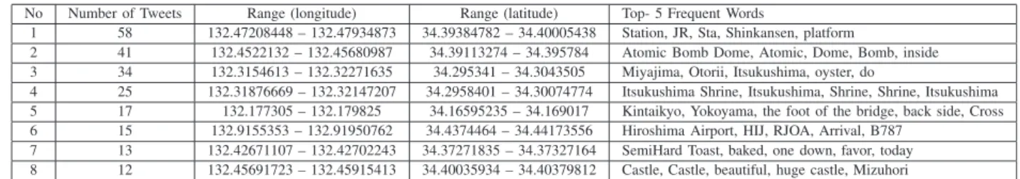
1 58 132.47208448 – 132.47934873 34.39384782 – 34.40005438 Station, JR, Sta, Shinkansen, platform

2 41 132.4522132 – 132.45680987 34.39113274 – 34.395784 Atomic Bomb Dome, Atomic, Dome, Bomb, inside

3 34 132.3154613 – 132.32271635 34.295341 – 34.3043505 Miyajima, Otorii, Itsukushima, oyster, do

4 25 132.31876669 – 132.32147207 34.2958401 – 34.30074774 Itsukushima Shrine, Itsukushima, Shrine, Shrine, Itsukushima 5 17 132.177305 – 132.179825 34.16595235 – 34.169017 Kintaikyo, Yokoyama, the foot of the bridge, back side, Cross 6 15 132.9155353 – 132.91950762 34.4374464 – 34.44173556 Hiroshima Airport, HIJ, RJOA, Arrival, B787

7 13 132.42671107 – 132.42702243 34.37271835 – 34.37327164 SemiHard Toast, baked, one down, favor, today 8 12 132.45691723 – 132.45915413 34.40035934 – 34.40379812 Castle, Castle, beautiful, huge castle, Mizuhori

as follows. Let keyi denote all words in dti of the i-th

georeferenced document: keyi = {ki,1, ki,2,· · ·, ki,nk(i)}, where ki ∈wi, ki,j ∈ K, and K is a set of all keywords

included inW. The keyword-based Simpson’s coefficient is defined as follows:

ksim(gdi, gdj) =

|keyi∩keyj| |min(keyi, keyj)|

. (3)

We defined a new function describing the similarity be-tween georeferenced documents that is a trade-off bebe-tween the word-based and keyword-based Simpson’s coefficients. This similarity function simis defined as follows:

sim(gdi, gdj) =w1 × wsim(gdi, gdj)

+ w2×ksim(gdi, gdj), (4)

where, w1+w2= 1.0. Ifw1 andw2 are set to 1.0 and 0.0, respectively, the keyword-based similarity function uses only word similarities. Conversely, Ifw1andw2are set to 0.0 and 1.0, respectively, the keyword-based similarity function uses only keyword similarities.

In the example described above, suppose that w1 = 0.5 and w2 = 0.5. In this case, the return values of wsim(gdi, gdj) and ksim(gdi, gdj) are 0.25 and 1.0,

re-spectively. Thus, the return value of the keyword-based sim-ilarity functionsimis0.5×0.25+0.5×1.0 = 0.6125. Based on this new similarity metric, the georeferenced documents gd1 and gd2, both of which included the local topic of “Itsukushima Shrine,” were determined to be similar to each other.

V. EXPERIMENTALRESULTS

To evaluate the (ǫ, σ)-density-based spatial clustering al-gorithm, we used an actual GDS composed of crawling

geo-tagged tweets on the Twitter site. In total, we collected 480,000 geo-tagged tweets from the site using its API from November 2011 to February 2012. In the experiments, we evaluate each in the dataset extracted from Hiroshima, Kyoto and Fukuoka from all geo-tagged tweets. We compared the results obtained using the (ǫ, σ)-density-based spatial clustering algorithm with those obtained using DBSCAN.

The parameters of DBSCAN were set to ǫ = 500m, whereas those of the (ǫ, σ)-density-based spatial clustering algorithm were set to ǫ = 500m, σ = 0.7. In accordance with the size of the dataset,M inDocwere set to 5, 10 and 15 in Hiroshima, Fukuoka and Kyoto respectively. Moreover, we used two types of the keyword-based similarity functions. In the first, which we refer to as the words-based method, the weight parameters w1 and w2 were set to 1.0 and 0.0, respectively. In the second, which we refer to as the keywords-based method, the weight parametersw1 andw2 were set to 0.5 and 0.5, respectively. We ranked the spatial clusters on the basis of the number of tweets included in each spatial cluster.

Tables from I to IX show the characteristics of the extracted spatial clusters, ranked by number of tweets, in Hiroshima, Kyoto and Fukuoka. In addition to the number of tweets, these tables also show the range of longitude and latitude for each spatial cluster, and the top 5 most frequent words in each spatial cluster, although words relevant to addresses (such as “Hiroshima” and “city”) were excluded.

(6)

TABLE IV

CLUSTERING RESULTS USINGDBSCANINKYOTO

1 8662 135.704244 – 135.80446464 34.94904073 – 35.06463114 shop, station, Mr/Ms, today, here 2 540 135.66452265 – 135.71345762 35.00498584 – 35.02707 Ranzan, cross, Tsukihashi, temple, Tenryu 3 198 135.55300055 – 135.58462697 34.801093 – 34.82376059 shop, Hankyu, station, Ibaraki-shi station, JR 4 174 135.85209595 – 135.88936967 34.99814065 – 35.01452177 Lake Biwa, shop, station, Komeda coffee shop, today

5 170 135.804991 – 135.83872 34.97368364 – 34.99499243 No, Marufuku, sign, station, JR

6 137 135.66272989 – 135.68484137 34.873768 – 34.89769033 station, years, stay, this, come

7 131 135.609333 – 135.63310402 34.841202 – 34.85899847 today, shop, Takatsuki-shi station, Hankyu, Mr/Ms 8 131 135.7506116 – 135.7723364 34.92495801 – 34.946655 Tanbabashi, shop, Sta, station, liquor

TABLE V

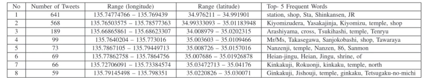
CLUSTERING RESULTS USING THE WORDS-BASED METHOD INKYOTO

1 641 135.74774766 – 135.769439 34.976211 – 34.991901 station, shop, Sta, Shinkansen, JR

2 568 135.76503575 – 135.78577363 34.99333093 – 35.01183948 Kiyomizudera, Yasakajinja, Kiyomizu, temple, shop 3 189 135.66865861 – 135.68623307 34.008979 – 35.0202315 Arashiyama, cross, Tsukihashi, temple, Tenryu

4 99 135.7640204 – 135.773016 35.003603 – 35.0109466 Mr/Ms, Takasegawa, Sanjokobashi, shop, Tawaraya

5 73 135.7867105 – 135.79449713 35.008726 – 35.0157016 Nanzenji, temple, Nanzen, 86, Sanmon

6 69 135.77862758 – 135.7864756 35.007686 – 35.01926878 Heian-jingu, Heian, Jingu, shrine, of 7 66 135.72706091 – 135.73384574 35.03472713 – 35.04176 Kinkakuji, Rokuonji, kinkaku, temple, north

8 59 135.79145498 – 135.798351 35.0220826 – 35.030071 Ginkakuji, Jishouji, temple, ginkaku, Tetsugaku-no-michi

TABLE VI

CLUSTERING RESULTS USING THE KEYWORDS-BASED METHOD INKYOTO

1 316 135.74927 – 135.7691693 34.980986 – 34.99070358 station, Sta, Shinkansen, JR, tower

2 116 135.77508884 – 135.78573167 34.9928148 – 34.99856858 Kiyomizudera, Kiyomizu, stage, temple, night

3 91 135.6725556 – 135.6854594 35.01031 – 35.0202315 Tsukihashi, cross, Arashiyama, fallen leaves, Nakanoshima

4 62 135.771915 – 135.780482 35.002736 – 35.0049482 Yasakajinja, Yasaka, Shrine, Higashiyama, 625

5 60 135.72706091 – 135.733314 35.03863312 – 35.04176 Kinkakuji, Rokuonji, kinkaku, temple, north

6 46 135.79145498 – 135.798351 35.0242942 – 35.030071 Ginkakuji, Jishouji, Ginkaku, temple, person

7 38 135.7691276 – 135.7788384 35.00226635 – 35.0104773 Minami-za, four, jo, here, cold

8 35 135.7713161 – 135.775702 34.966555 – 34.96792031 Fushimiinari-taisha, taisha, Fushimi, shrine, inari

DBSCAN in downtown Hiroshima on the Google Map. It is clear that the density of posted tweets is high in down-town Hiroshima, which can be attributed to the abundant population. Therefore, this area was extracted as one spatial cluster including several local topics. Similarly, Fig. 5(a) and Fig. 6(a) illustrate the locations of tweets of spatial clusters extracted using DBSCAN in downtown Kyoto and Fukuoka on the Google Map respectively. These areas were also extracted as one spatial cluster including several local topics. Accordingly, DBSCAN was unable to recognize semantically separated spatial clusters.

Tables II and III present spatial clusters extracted using the proposed the words-based and keywords-based methods in Hiroshima, respectively. Similarly, Tables V and VI present extracted spatial clusters in Kyoto, and Tables VIII and IX present extracted spatial clusters in Fukuoka, respectively. It is clear that, in contrast to DBSCAN, the(ǫ, σ)-density-based spatial clustering algorithm was able to recognize multiple spatial clusters. Fig. 4, Fig. 5 and Fig. 6 (b) and (c) illustrate the locations of tweets of spatial clusters extracted using the proposed(ǫ, σ)-density-based spatial clustering algorithm located in downtown Hiroshima, Kyoto and Fukuoka in the Google Map respectively.

The (ǫ, σ)-density-based spatial clustering algorithm was able to recognize semantically separated spatial clusters; however, cluster 1 in Table II includes local topics in downtown Hiroshima. For example, many tweets related to “Okonomiyaki restaurant,” “streetcars,” and “Hiroshima’s oyster” were found; these tweets included the same address. Therefore, these tweets were determined similar when using the words-based method. However, this spatial cluster was not extracted using the keywords-based method.

The keywords-based method was compared with the words-based method by checking the contents of extracted spatial clusters. The extracted spatial clusters referred to as 4 in Table II and 2 in Table III are associated broadly with the same topic, related to “Atomic Bomb Dome.” However, the number of tweets extracted by the keywords-based method is six fewer than the words-based method. We checked these six tweets manually and found that their topic was “Atomic Bomb Dome Sta.” This result indicates that the keywords-based method can recognize spatial clusters more accurately than the words-based method.

We also compared the keywords-based method with the words-based method in Kyoto. The extracted spatial clusters referred to as 2 in Table V and 2 in Table VI are associated broadly with the same topic, related to “Kiyomizudera.” However, there is a large difference in the number of tweets in spatial clusters (568 tweets when using the words-based method, and 116 tweets when using the keywords-based method). Tweets of the spatial cluster using the words-based method are related to “Yasakajinja,” “Gion” and “Chion-in Temple” and so on. When using the keywords-based method, spatial clusters of these tweets were extracted separately (Cluster number 4, 11 and 22). In other words, the keywords-based method was able to separate spatial clusters by the contents of tweets compared with the words-based method.

(7)

TABLE VII

CLUSTERING RESULTS USINGDBSCANINFUKUOKA

1 6590 130.3392691 – 130.462255 33.5436319 – 33.63534791 shop, station, today, Tenjin, Mr/Ms 2 358 130.49434885 – 130.53703863 33.28378128 – 33.328096 Ramen, green, 2, professional, rice

3 268 130.51297552 – 130.53861 33.5071187 – 33.52296235 Dazaifu-Tenmangu, shop, Omotesando, Coffee, Starbucks 4 249 130.28752904 – 130.32005137 33.23811636 – 33.272056 Mr/Ms, today, shop, come, station

5 216 130.3111012 – 130.341107 33.5516335 – 33.59836152 shop, today, come, udon, Ramen

6 140 130.46180067 – 130.49610531 33.51233611 – 33.55466409 shop, today, Mr/Ms, Onojo, Dazaifu 7 103 130.41597282 – 130.44754509 33.64563772 – 33.666828 shop, today, pic, east, station

8 102 129.9806848 – 129.9806848 33.4402852 – 33.46179803 center, love, do, station, Mr/Ms

TABLE VIII

CLUSTERING RESULTS USING THE WORDS-BASED METHOD INFUKUOKA

1 565 130.4099839 – 130.4282586 33.58518764 – 33.59547401 station, JR, shop, Sta, illumination 2 396 130.39071769 – 130.40485734 33.58483201 – 33.59497558 Tenjin, shop, Ramen, today, building 3 131 130.4430685 – 130.45001799 33.59445983 – 33.601311 Fukuoka Airport, Airport, Fukuoka, FUK, RJFF 4 99 130.53122 – 130.53503418 33.51945473 – 33.52163006 Dazaifu-Tenmangu, shop, Omotesando, Coffee, Starbucks 5 82 130.40722712 – 130.41402031 33.58813125 – 33.59157254 Canal City Hakata, shop, buying, please, Canal 6 33 130.40828578 – 130.41357207 33.58766034 – 33.59239561 Canal City, shop, Washington, hotel, Ramen 7 33 130.40998907 – 130.41205231 33.58848247 – 33.58938699 buying, please, model, pretty, happy

8 29 130.3582136 – 130.3644506 33.59281572 – 33.597106 dome, Yahoo!, JAPAN, arrival, today

TABLE IX

CLUSTERING RESULTS USING THE KEYWORDS-BASED METHOD INFUKUOKA

1 322 130.41012816 – 130.4253221 33.58522654 – 33.594532 station, Sta, JR, illumination, Hakataekichuogai 2 102 130.4430685 – 130.45001799 33.59445983 – 33.601311 Fukuoka Airport, Airport, Fukuoka, FUK, RJFF 3 91 130.53287258 – 130.53503418 33.51945473 – 33.52153733 Dazaifu-Tenmangu, Omotesando, Coffee, Starbucks, shop 4 66 130.40722712 – 130.41519389 33.5861906 – 33.59157254 buying, please, shop, Canal City Hakata, pretty 5 37 130.3953001 – 130.40504301 33.58575373 – 33.59342454 Tenjin, shop, exist, person, come

6 35 130.871513 – 130.872631 33.816385 – 33.816562 KTC, 20, cafeteria, building number, weather

7 34 130.396545 – 130.40203661 33.58680983 – 33.59286041 Tenjin, shop, 11, Tenjintikagai, 10 8 28 130.41031294 – 130.41402031 33.58883194 – 33.5913509 Canal City Hakata, City, Hakata, Canal, 25

related to “Canal City Hakata”, which is a big shopping mall in Fukuoka city. In this case, spatial clusters referred to as 5 and 7 in Table VIII and 4 and 8 in Table IX are advertising, they are tweeted by “Canal City Hakata.” In our future work, it is necessary to weigh lower weight to tweets posted by one user.

The extracted spatial cluster referred to as 8 in Table VIII, related to “Fukuoka Yahoo! JAPAN dome.” However, contents of the tweets are different. For example, there are tweets of baseball game, entertainment and live concert. By words of “Yahoo!,” “JAPAN” and “dome,” these tweets were determined similar. Even when using the keyword-based method, spatial cluster of cluster number 15 and Number of Tweets 19 are extracted. From these results, we should improve the precision of the similarity of tweet calculation in the future.

VI. CONCLUSION

In this paper, we proposed a novel spatial clustering algorithm, referred to as the(ǫ, σ)-density-based spatial clus-tering algorithm, for extracting “attractive” local-area topics in georeferenced documents. The proposed density-based spatial clustering algorithm can recognize both spatially and semantically separated spatial clusters. There we can extract local-area topics as (ǫ, σ)-density-based spatial clusters. To evaluate our proposed density-based spatial clustering algo-rithm, we used geo-tagged tweets posted on the Twitter site. The experimental results show that the (ǫ, σ)-density-based spatial clustering algorithm can extract “attractive” local-area topics as (ǫ, σ)-density-based spatial clusters. In our future work, we intend to develop an online algorithm to extract (ǫ, σ)-density-based spatial clusters in real-time.

ACKNOWLEDGMENT

This work was supported by Hiroshima City University Grant for Special Academic Research (General Studies) and JSPS KAKENHI Grant Number 26330139.

REFERENCES

[1] M. Naaman, “Geographic information from georeferenced social me-dia data,”SIGSPATIAL Special, vol. 3, no. 2, pp. 54–61, jul 2011. [2] S. Van Canneyt, S. Schockaert, O. Van Laere, and B. Dhoedt,

“De-tecting places of interest using social media,” inProceedings of the The 2012 IEEE/WIC/ACM International Joint Conferences on Web Intelligence and Intelligent Agent Technology - Volume 01, ser. WI-IAT ’12, 2012, pp. 447–451.

[3] H. Yang, S. Chen, M. R. Lyu, and I. King, “Location-based topic evolution,” inProceedings of the 1st international workshop on Mobile location-based service, ser. MLBS ’11, 2011, pp. 89–98.

[4] D. J. Crandall, L. Backstrom, D. Huttenlocher, and J. Kleinberg, “Mapping the world’s photos,” inProceedings of the 18th international conference on World wide web, ser. WWW ’09, 2009, pp. 761–770. [5] T. Sakaki, M. Okazaki, and Y. Matsuo, “Earthquake shakes twitter

users: real-time event detection by social sensors,” inProceedings of the 19th international conference on World wide web, ser. WWW ’10, 2010, pp. 851–860.

[6] T. Sakai, K. Tamura, and H. Kitakami, “A new density-based spatial clustering algorithm for extracting attractive local regions in georefer-enced documents,” inProceedings of The International MultiConfer-ence of Engineers and Computer Scientists 2014, IMECS 2014, 12-14 March, 2014, Hong Kong, pp. 360–365.

[7] M. Ester, H.-P. Kriegel, J. Sander, and X. Xu, “A density-based algorithm for discovering clusters in large spatial databases with noise,” inSecond International Conference on Knowledge Discovery and Data Mining, E. Simoudis, J. Han, and U. M. Fayyad, Eds. AAAI Press, 1996, pp. 226–231.

[8] M. F. Goodchild, “Citizens as voluntary sensors: Spatial data infras-tructure in the world of web 2.0,”International Journal of Spatial Data Infrastructures Research, vol. 2, pp. 24–32, 2007.

(8)

(a) DBSCAN (b) Words-based method (c) Keywords-based method

Fig. 4. Data plots for downtown Hiroshima on Google Map

Fig. 5. Data plots for downtown Kyoto on Google Map

Fig. 6. Data plots for downtown Fukuoka on Google Map

[10] J. Sander, M. Ester, H.-P. Kriegel, and X. Xu, “Density-based cluster-ing in spatial databases: The algorithm gdbscan and its applications,” Data Mining and Knowledge Discovery, vol. 2, no. 2, pp. 169–194, jun 1998.

[11] K. Tamura and T. Ichimura, “Density-based spatiotemporal clustering algorithm for extracting bursty areas from georeferenced documents,” inProceedings of the IEEE International Conference on System, Man, and Cybernetics, SMC 2013, 2013, pp. 2079-2084.

[12] S. Kisilevich, F. Mansmann, and D. Keim, “P-dbscan: a density based clustering algorithm for exploration and analysis of attractive areas using collections of geo-tagged photos,” in Proceedings of the 1st International Conference and Exhibition on Computing for Geospatial Research & Application, ser. COM.Geo ’10, 2010, pp. 38:1–38:4. [13] K. Watanabe, M. Ochi, M. Okabe, and R. Onai, “Jasmine: a real-time

local-event detection system based on geolocation information propa-gated to microblogs,” inProceedings of the 20th ACM international conference on Information and knowledge management, ser. CIKM ’11, 2011, pp. 2541–2544.

[14] R. Lee and K. Sumiya, “Measuring geographical regularities of crowd behaviors for twitter-based geo-social event detection,” inProceedings

of the 2nd ACM SIGSPATIAL International Workshop on Location Based Social Networks, ser. LBSN ’10, 2010, pp. 1–10.

[15] A. Jaffe, M. Naaman, T. Tassa, and M. Davis, “Generating summaries and visualization for large collections of geo-referenced photographs,” inProceedings of the 8th ACM international workshop on Multimedia information retrieval, ser. MIR ’06, pp. 89–98.

[16] T. Rattenbury, N. Good, and M. Naaman, “Towards automatic extrac-tion of event and place semantics from flickr tags,” inProceedings of the 30th annual international ACM SIGIR conference on Research and development in information retrieval, ser. SIGIR ’07, pp. 103–110. [17] K. Yanai, K. Yaegashi, and B. Qiu, “Detecting cultural differences

using consumer-generated geotagged photos,” in Proceedings of the 2nd International Workshop on Location and the Web, ser. LOCWEB ’09, 2009, pp. 12:1–12:4.